If you frequently analyze data in Excel, you may come across empty cells before the actual values. Instead of removing these cells, you can get the position or even the value of the first non-blank cell with formulas. In this article, we are going to show you how to find the first non-blank cell in a range in Excel.
Formula
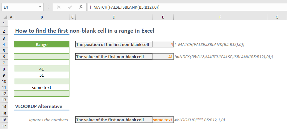
Get the value: {=INDEX(range,MATCH(FALSE,ISBLANK(range),0))}
* range is the reference from the work range
How it works
Excel doesn’t have a built-in formula to find the first non-blank cell in a range. However, there is ISBLANK function which checks a cell and returns a Boolean value according to its content. The function returns TRUE if cell is blank, FALSE otherwise. Thus, finding the first FALSE value means to find the first non-blank cell.
MATCH function can help to locate FALSE value. Once the position is in hand, you can use it with INDEX function to get the result.
The problem is ISBLANK function only works with a single cell. You need to use a helper column to populate TRUE and FALSE values which doesn’t sound practical. Instead, you can use an array function and not need the helper column.
Use the reference of your range of values in the ISBLANK function. This action will return an array of Boolean values. The first FALSE value indicates the position of the first non-blank cell in the range. Wrap the function with either MATCH or INDEX-MATCH combo to get the position or the value respectively.
Use Ctrl + Shift + Enter key combination instead of regular Enter key to evaluate the formula as an array formula.
![]()