Volume 2 - International Environmental Modelling and Software ...

Complexity and Integrated 

Resources Management 

Transactions 

of the 2nd Biennial Meeting of the 

International Environmental Modelling 

and Software Society 

Editors 

Claudia Pahl-Wostl 

Sonja Schmidt 

Andrea E. Rizzoli 

Anthony J. Jakeman 

IEMSs 2004 – 14-17 June 2004, 

University of Osnabrück, Germany

Complexity and Integrated Resources Management - Transactions of the 2nd Biennial 

Meeting of the International Environmental Modelling and Software Society 

Volume Editors 


Sonja Schmidt 

Institut für Umweltsystemforschung 

Universität Osnabrück 

Artilleriestr. 34 

D 49076 Osnabrück, Germany 

Andrea E. Rizzoli 

IDSIA Istituto Dalle Molle di studi sull'intelligenza artificiale 

Galleria 2 

CH 6928 Manno, Switzerland 

Anthony J. Jakeman 

The Centre for Resource and Environmental Studies (Bldg 43) 

The Australian National University 

ACT 0200, Canberra, Australia 

Each paper in this volume was refereed by an Editor, a member of the Editorial Board and 

two anonymous referees. 

The copyright of all papers is an exclusive right of the authors. No work can be reproduced 

without written permission of the authors. 

Responsibility for the contents of these papers rests upon the authors and not on the 

International Environmental Modelling and Software Society. 

ISBN 88-900787-1-5 

iEMSs 2004 

Published by the International Environmental Modelling and Software Society (iEMSs) 

President: Anthony J. Jakeman. 

Address: iEMSs, c/- IDSIA, Galleria 2, 6928 Manno, Switzerland 

Email: secretary@iemss.org 

Website: http://www.iemss.org 

II 

Typeset in Como (Italy) by SEA, Servizi Editoriali Associati

IEMSs 2004 – 14-17 June 2004, 

University of Osnabrück, Germany 

Complexity and Integrated Resources 

Management Transactions of the 2nd Biennial 

Meeting of the International Environmental 

Modelling and Software Society 

Claudia Pahl-Wostl, Sonja Schmidt, Andrea 

E. Rizzoli, Anthony J. Jakeman ( E d i t o r s ) 

Co-editors 

David Batten Keith Jeffery Dale S. Rothman 

Michel Blind Kostas Karatzas Miquel Sànchez-Marrè 

Felix Chan Markus Knoflacher Dragan Savic 

Barry Croke Peter Krause Huub Scholten 

Wolfgang-Albert Flügel Christine Lim Boris Schröder 

Carlo Giupponi Ian Littlewood Jan Sendzimir 

Romy Greiner Michael Matthies Ralf Seppelt 

Carlo Gualtieri Michael McAleer Achim Sydow 

Nigel Hall Dragutin T. Mihailovic Hilde Passier 

Matt Hare Les Oxley David Post 

Reinout Heijungs Jens C. Refsgaard Peter Vanrolleghem 

Stefanie Hellweg 

Otto Richter 

Suhejla Hoti 

Michela Robba 

Organizers 

The conference has been organized by iEMSs 

(the International Environmental Modelling and Software Society) in cooperation with: 

Harmoni-CA (Concerted Action on Harmonizing Modelling Tools for River Basin Management) 

TIAS (Integrated Assessment Society) 

IAHS (International Association of Hydrological Sciences) 

BESAI (Binding Environmental Sciences and Artificial Intelligence) 

MODSS International Conference on Multi-objective Decision Support Systems for Land, 

Water and Environmental Management 

ISESS International Symposium on Environmental Software Systems 

ERCIM the European Research Consortium for Informatics and Mathematics 

Local Organizers 

The local organization of the conference has been managed by: 

DBU (German Environmental Foundation) 

USF (Institute of Environmental Systems Research, University of Osnabrück) 

III

Editorial 

Dear Reader, 

The 2nd Biennial Meeting of the International Environmental Modelling and Software Society (iEMSS 2004) was dedicated 

to the theme: Complexity and Integrated Resources Management”, a very topical theme given the increasing complexity 

of contemporary resource management problems and the increasing uncertainties from global change. The meeting 

assembled nearly 300 researchers from all over the globe and from a wide range of disciplines. Presentations 

discussed latest developments in modelling methodologies and software tools applied to different areas of resources 

management. Contributions provided evidence of the important role of models to improve our understanding of the complexity 

of socio-ecological systems and to develop appropriate management strategies. Increasing attention was paid 

to the role of stakeholders in model development and application and to a new role for models in processes of social 

learning in participatory resources management. 

The conference took place in the facilities of the German Environmental Foundation in Osnabrück. The ambience of 

these low-energy buildings, designed to minimise their impact on the environment, was well suited to the conference 

theme and their open and flexible structure facilitated intense discussions and exchange not only during but also 

between sessions. 

I hope that readers will share the excitement of conference participants when browsing through the conference proceedings 

and reading some of the papers in more detail. Interested readers are advised to consult the journals 

Environmental Modelling and Software and Ecological Modelling and Advances in Geosciences where special issues 

emanating from this conference will be published. We also look forward to the third biennial meeting, iEMSs 2006, which 

will be held in Burlington, Vermont, USA (see http://www.iemss.org/iemss2006). 

October 2004 


The International Environmental Modelling and Software Society acknowledges gratefully the assistance of the 

following people in realizing the iEMSs 2004 conference: 

• Claudia Pahl-Wostl for convening the conference 

• Sonja Schmidt for organising the conference 

• Andrea Rizzoli for the web-based conference management tool, creating and updating the conference website 

and for expert and technical advice 

• all session organizers and reviewers 

• Antje Braeuer and Georg Johann for supporting the organisation whenever and wherever necessary 

• all members of the Institute of Environmental Systems Research and the department of resource flow management 

for supporting iEMSs 2004, especially Ilke Borowski, Frank Hilker, Maja Schlüter and Dominik Reusser 

• all members of ZUK “Zentrum für Umweltkommunikation“ of the German Environmental Foundation 

IV

TABLE OF CONTENTS 

iEMSs 2004 sessions (part two) 

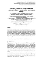
Environmental Informatics Towards Citizen-centred Electronic 

Information Services: the Urban Environment Example 

Using FLOSS towards Building Environmentale Information 

K. Karatzas, A. Masouras . . . . . . . . . . . . . . . . . . . . . . . . . . . . . . . . . . . . . . . . . . . . . . . . . . . . . . . . . . . . . . . . . . . . . .p. 525 

Applying agent technologyin Environmental Management Systems underreal-time constraints 

I.N. Athanasiadis, P.A. Mitkas . . . . . . . . . . . . . . . . . . . . . . . . . . . . . . . . . . . . . . . . . . . . . . . . . . . . . . . . . . . . . . . . . .p. 531 

Supporting the Strategic Objectives of Participative Water Resources Management; 

an Evaluation of the Performance of Four ICT Tools 

A. Swinford, B. McIntosh, P. Jeffrey . . . . . . . . . . . . . . . . . . . . . . . . . . . . . . . . . . . . . . . . . . . . . . . . . . . . . . . . . . .p. 537 

Web Services for Environmental Informatics 

E. Arauco, L. Sommaruga . . . . . . . . . . . . . . . . . . . . . . . . . . . . . . . . . . . . . . . . . . . . . . . . . . . . . . . . . . . . . . . . . . . . .p. 543 

Environmental Decision Support Systems 

Concepts of Decision Support for River Rehabilitation P. Reichert, M. Borsuk, M. Hostmann, 

S. Schweizer, C. Spörri, K. Tockner, B. Truffer . . . . . . . . . . . . . . . . . . . . . . . . . . . . . . . . . . . . . . . . . . . . . . . . . .p. 550 

Decision Making under Uncertainty in a Decision Support System for the Red River Inge 

A.T. de Kort, M.J. Booij . . . . . . . . . . . . . . . . . . . . . . . . . . . . . . . . . . . . . . . . . . . . . . . . . . . . . . . . . . . . . . . . . . . . . . . .p. 556 

Development of a GIS-based Decision Support Tool for Integrated Water Resources Management in 

Southern Africa 

M. Märker, K.Bongartz, W.A. Flügel . . . . . . . . . . . . . . . . . . . . . . . . . . . . . . . . . . . . . . . . . . . . . . . . . . . . . . . . . . . .p. 562 

Possible Courses: Multi-Objective Modelling and Decision Support Using a Bayesian Network 

Approximation to a Nonpoint Source Pollution Model 

D. Swayne, J. Shi . . . . . . . . . . . . . . . . . . . . . . . . . . . . . . . . . . . . . . . . . . . . . . . . . . . . . . . . . . . . . . . . . . . . . . . . . . . . .p. 568 

V

A Spatial DSS for South Australia's Prawn Fisheries. Using Historic Knowledge Towards Environmental 

and Economical Sustainability 

B. Ostendorf, N. Carrick . . . . . . . . . . . . . . . . . . . . . . . . . . . . . . . . . . . . . . . . . . . . . . . . . . . . . . . . . . . . . . . . . . . . . . .p. 574 

Optimum Sustainable Water Management in an Urbanizing River Basin in Japan, Based on Integrated 

Modelling Techniques 

E. Kudo, M. Ostrowski . . . . . . . . . . . . . . . . . . . . . . . . . . . . . . . . . . . . . . . . . . . . . . . . . . . . . . . . . . . . . . . . . . . . . . . . .p. 580 

Application of a GIS-based Simulation Tool to Analyze and Communicate Uncertainties in Future Water 

Availability in the Amudarya River Delta 

M. Schlüter, N. Rüger . . . . . . . . . . . . . . . . . . . . . . . . . . . . . . . . . . . . . . . . . . . . . . . . . . . . . . . . . . . . . . . . . . . . . . . . .p. 586 

Integration of MONERIS and GREAT-ER in the Decision Support System for the German Elbe River Basin 

J. Berlekamp, N. Graf, O. Hess, S. Lautenbach, S. Reimer, M. Matthies . . . . . . . . . . . . . . . . . . . . . . . . . . . . . . . .p . 5 9 3 

An integrated tool for water policy in agriculture 

G.M. Bazzana . . . . . . . . . . . . . . . . . . . . . . . . . . . . . . . . . . . . . . . . . . . . . . . . . . . . . . . . . . . . . . . . . . . . . . . . . . . . . . . . .p. 599 

Towards a Decision Support System for Real Time Risk Assessment of Hazardous Material Transport on 

Road 

D. Giglio, R. Minciardi, D. Pizzorni, R. Rudari, R. Sacile, A. Tomasoni, E. Trasforini . . . . . . . . . . . . . .p. 605 

Appropriate Modelling in DSSs for River Basin Management 

Y. Xu, M.J. Booij . . . . . . . . . . . . . . . . . . . . . . . . . . . . . . . . . . . . . . . . . . . . . . . . . . . . . . . . . . . . . . . . . . . . . . . . . . . . . . .p. 611 

Water Management, Public Participation and Decision Support Systems: the MULINO Approach 

J. Feás, C. Giupponi, P. Rosato . . . . . . . . . . . . . . . . . . . . . . . . . . . . . . . . . . . . . . . . . . . . . . . . . . . . . . . . . . . . . . . .p. 617 

A Dual-scale Modelling approach to Integrated Resource Management in East and South-east Asia: 

Challenges and Potential solutions 

R. Rötter, M. van den Berg, H. Hengsdijk, J. Wolf, M. van Ittersum, H. van Keulen, E.O. Agustin, T. T. Son, 

N.X. Lai, W. Guanghuo, A.G. Laborte . . . . . . . . . . . . . . . . . . . . . . . . . . . . . . . . . . . . . . . . . . . . . . . . . . . . . . . . . . . . . . . . . .p . 6 2 3 

The role of Multi-Criteria Decision Analysis in a DEcision Support sYstem for REhabilitation 

of contaminated sites (the DESYRE software) 

C. Carlon, S. Giove, P. Agostini, A. Critto, A. Marcomini . . . . . . . . . . . . . . . . . . . . . . . . . . . . . . . . . . . . . . .p. 629 

ICT Requirements for an 'evolutionary' development of WFD compliant River Basin Management Plans 

M. Blind . . . . . . . . . . . . . . . . . . . . . . . . . . . . . . . . . . . . . . . . . . . . . . . . . . . . . . . . . . . . . . . . . . . . . . . . . . . . . . . . . . . . . . .p. 635 

DAWN:A platform for evaluating water-pricing policies using a software agent society 

I.N. Athanasiadis, P. Vartalas, P.A. Mitkasa . . . . . . . . . . . . . . . . . . . . . . . . . . . . . . . . . . . . . . . . . . . . . . . . . . . . .p. 643 

Empirical Evaluation of Decision Support Systems: Concepts and an Example for Trumpeter Swan 

Management 

R.S. Sojda . . . . . . . . . . . . . . . . . . . . . . . . . . . . . . . . . . . . . . . . . . . . . . . . . . . . . . . . . . . . . . . . . . . . . . . . . . . . . . . . . . . .p. 649 

An integrated modelling approach to conduct multi-factorial analyses on the impacts 

of climate change on whole-farm systems 

M. Rivington, G. Bellocchi, K.B. Matthews, K. Buchan, M. Donatelli . . . . . . . . . . . . . . . . . . . . . . . . . . . .p. 656 

VI

Some Methodological Concepts to Analyse the Role of IC-tools in Social Learning Processes 

P. Maurel, F. Cernesson, N, Ferrand, M. Craps, P. Valkering . . . . . . . . . . . . . . . . . . . . . . . . . . . . . . . . . . . .p. 662 

Tools to Think With? Towards Understanding the Use and Impact of Model-Based Support Tools 

B.S. McIntosh, R.A.F. Seaton, P. Jeffrey . . . . . . . . . . . . . . . . . . . . . . . . . . . . . . . . . . . . . . . . . . . . . . . . . . . . . . .p. 668 

Uncertainty in the Water Framework Directive: Implications for Economic Analysis 

J. Mysiak, K. Sigel . . . . . . . . . . . . . . . . . . . . . . . . . . . . . . . . . . . . . . . . . . . . . . . . . . . . . . . . . . . . . . . . . . . . . . . . . . . . .p. 674 

An Interactive Spatial Optimisation Tool for Systematic Landscape Restoration B.A. Bryana, L.M. Perryb, 

D. Gerner, B. Ostendorf, N.D. Crossman . . . . . . . . . . . . . . . . . . . . . . . . . . . . . . . . . . . . . . . . . . . . . . . . . . . . . . .p. 680 

Assessing the Feasibility of Using Radar Satellite Data to Detect Flood Extent and Floodplain Structures 

Edith Stabel . . . . . . . . . . . . . . . . . . . . . . . . . . . . . . . . . . . . . . . . . . . . . . . . . . . . . . . . . . . . . . . . . . . . . . . . . . . . . . . . . . .p. 686 

Optimal Groundwater Exploitation and Pollution Control 

A. Bagnera, M. Massabò, R. Minciardi, L. Molini, M. Robba, R. Sacile . . . . . . . . . . . . . . . . . . . . . . . . . . . . .p. 693 

Towards an Environmental DSS basedon Spatio-Temporal Markov Chain Approximation 

G. Balent, M. Deconchat, S. Ladet, R. Martin-Clouaire, R. Sabbadin . . . . . . . . . . . . . . . . . . . . . . . . . . . . . .p. 699 

Regional Dynamic Modelling 

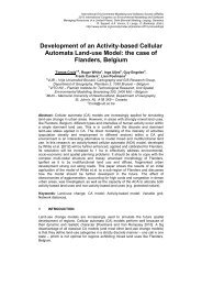
Land Use and Hydrological Management: ICHAM, an Integrated Model at a Regional Scale in 

Northeastern Thailand 

N. Hall, R. Lertsirivorakul, R. Gre i n e r, S. Yongvanit, A. Yuvaniyama, R. Lastf, W. Milne-Homef . . . . . . . .p. 705 

Forecasting Municipal Solid Waste Generation in MajorEuropean Cities 

P. Beigl, G. Wassermann, F. Schneider, S. Salhofer . . . . . . . . . . . . . . . . . . . . . . . . . . . . . . . . . . . . . . . . . . . .p. 711 

Real Time Optimal Resource Allocation in Natural Hazard Management 

P. Fiorucci, F. Gaetani, R. Minciardi, R. Sacile, E. Trasforini . . . . . . . . . . . . . . . . . . . . . . . . . . . . . . . . . . . . .p. 717 

Combining Dynamic Economic Analysis and Environ-mental Impact Modelling: Addressing Uncertainty 

and Complexity of Agricultural Development 

H. Lehtonen, I. Bärlund, S. Tattari, M. Hilden . . . . . . . . . . . . . . . . . . . . . . . . . . . . . . . . . . . . . . . . . . . . . . . . . . .p. 723 

Simulation of Water and Carbon Fluxes in Agro- and forest Ecosystems at the Regional Scale 

J. Post, V. Krysanova, F. Suckow . . . . . . . . . . . . . . . . . . . . . . . . . . . . . . . . . . . . . . . . . . . . . . . . . . . . . . . . . . . . . .p. 730 

An Integrated Geomorphological and Hydrogeological MMS Modelling Framework for a Semi-Arid 

Mountain Basin in the High Atlas, Southern Morocco 

C. de Jong, R. Machauer, B. Reichert, S. Cappy, R. Viger, G. Leavesley . . . . . . . . . . . . . . . . . . . . . . . .p. 736 

Anticipated Effects of Re-Allocation of Intensive Livestock in Sandy Areas in the Netherlands 

A. van Wezel, J.D. van Dam, P. Cleij . . . . . . . . . . . . . . . . . . . . . . . . . . . . . . . . . . . . . . . . . . . . . . . . . . . . . . . . . . .p. 742 

An Integrated System for the Forest Fires Dynamic Hazard Assessment Over a Wide Area 

P. Fiorucci, F. Gaetani, R. Minciardi . . . . . . . . . . . . . . . . . . . . . . . . . . . . . . . . . . . . . . . . . . . . . . . . . . . . . . . . . . . .p. 748 

VII

Scenario Development and Integrated Scenario Modelling 

Linking Narrative Storylines and Quantitative Models to Combat Desertification in the Guadalentín, Spain 

K. Kok, H. Van Delden . . . . . . . . . . . . . . . . . . . . . . . . . . . . . . . . . . . . . . . . . . . . . . . . . . . . . . . . . . . . . . . . . . . . . . . . .p. 754 

Integrated Assessment of Water Stress in Ceara, Brazil, under Climate Change Forcing 

M.S. Krol. P. van Oel . . . . . . . . . . . . . . . . . . . . . . . . . . . . . . . . . . . . . . . . . . . . . . . . . . . . . . . . . . . . . . . . . . . . . . . . . .p. 760 

From Narrative to Number: A Role for Quantitative Models in Scenario Analysis 

E. Kemp-Benedict . . . . . . . . . . . . . . . . . . . . . . . . . . . . . . . . . . . . . . . . . . . . . . . . . . . . . . . . . . . . . . . . . . . . . . . . . . . . .p. 765 

Scenario Reoptimization under Data Uncertainty 

P. Zuddas, G.M. Sechi, A. Manca . . . . . . . . . . . . . . . . . . . . . . . . . . . . . . . . . . . . . . . . . . . . . . . . . . . . . . . . . . . . . .p. 771 

Reliable and Valid Identification of a Small Number of Global Emission Scenarios 

O. Tietje . . . . . . . . . . . . . . . . . . . . . . . . . . . . . . . . . . . . . . . . . . . . . . . . . . . . . . . . . . . . . . . . . . . . . . . . . . . . . . . . . . . . . . .p. 777 

Simulating Global Feedbacks Between Sea Level Rise, Water for Agriculture and the Complex 

Socio-Economic Development of the IPCC Scenarios 

S. Werners, R. Boumans, L. Bouwer . . . . . . . . . . . . . . . . . . . . . . . . . . . . . . . . . . . . . . . . . . . . . . . . . . . . . . . . . . .p. 783 

Biocomplexity and Adaptive Ecosystem Management 

Principles of Human-Enviroment Systems (HES) Research 

R. Scholz, C. Binder . . . . . . . . . . . . . . . . . . . . . . . . . . . . . . . . . . . . . . . . . . . . . . . . . . . . . . . . . . . . . . . . . . . . . . . . . . .p. 791 

Addressing Sustainability, HIV-AIDS, and Water Resource Questions in Botswana 

M. Hellmuth, J. Sendzimir, D. Yates, K. Strzepek, W. Sanderson . . . . . . . . . . . . . . . . . . . . . . . . . . . . . . . . . . .p. 797 

Modelling Biocomplexity in the Tisza River Basin within a Participatory Adaptive Framework 

J. Sendzimir, P. Balogh, A. Vári . . . . . . . . . . . . . . . . . . . . . . . . . . . . . . . . . . . . . . . . . . . . . . . . . . . . . . . . . . . . . . . .p. 803 

Linking Hydrologic Modeling and Ecologic Modeling: An Application of Adaptive Ecosystem Management 

in the Everglades Mangrove Zone of Florida Bay 

J.C. Cline, J. Lorenz, E. Swain . . . . . . . . . . . . . . . . . . . . . . . . . . . . . . . . . . . . . . . . . . . . . . . . . . . . . . . . . . . . . . . . .p. 810 

On the Local Coexistence of Species in Plant Communities 

J. Yoshimura, K. Tainaka, T. Suzuki, M. Shiyomi . . . . . . . . . . . . . . . . . . . . . . . . . . . . . . . . . . . . . . . . . . . . . . . .p. 816 

Ecosystems as Evolutionary Complex Systems: A Synthesis of Two System-Theoretic Approaches Based 

on Boolean Network 

B. Fath, W. Grant . . . . . . . . . . . . . . . . . . . . . . . . . . . . . . . . . . . . . . . . . . . . . . . . . . . . . . . . . . . . . . . . . . . . . . . . . . . . . .p. 822 

Benthic Macroinvertebrates Modelling Using Artificial Neural Networks (ANN): 

Case Study of a Subtropical Brazilian River 

D. Pereira, M. de A. Vitola, O.C. Pedrollo, I.C. Junqueira, S.J. de Luca . . . . . . . . . . . . . . . . . . . . . . . . .p. 828 

Interspecific Segregation and Phase Transition in a Lattice Ecosystem with Intraspecific Competition 

K. Tainaka, M. Kushida, Y. Itoh, J. Yoshimura . . . . . . . . . . . . . . . . . . . . . . . . . . . . . . . . . . . . . . . . . . . . . . . . . .p. 834 

VIII

A Model of the Biocomplexity of Deforestation in Tropical Forest: Caparo Case Study 

R. Quintero, R. Barros, J. Dàvila, N. Moreno, G. Tonella, M. Ablan . . . . . . . . . . . . . . . . . . . . . . . . . . . . . . . . . .p. 840 

Developing Tools for Adaptive Integrated Water Resource Management in a Semi-Arid Region: 

Possibilities, Probabilities and Uncertainties 

D. Eisenhuth, J.B. Abad, A. Bonnet . . . . . . . . . . . . . . . . . . . . . . . . . . . . . . . . . . . . . . . . . . . . . . . . . . . . . . . . . . . .p. 846 

Ecological Modelling 

Stability Analyses of the 50/50 Sex Ratio Using Lattice Simulation 

Y. Itoh, J. Yoshimura, K. Tainaka . . . . . . . . . . . . . . . . . . . . . . . . . . . . . . . . . . . . . . . . . . . . . . . . . . . . . . . . . . . . . . .p. 852 

Reproductive Strategies of Marine Green Algae: the Evolution of Slight Anisogamy and Environmental 

Conditions of Habitat 

T. Togashi, T. Miyazaki, J. Yoshimura, J.L. Bartelt, P.A. Cox . . . . . . . . . . . . . . . . . . . . . . . . . . . . . . . . . . . . .p. 858 

Predicting Predation Efficiency of Biocontrol Agents: Linking Behavior of Individuals and Population 

Dynamics 

B. Tenhumberg . . . . . . . . . . . . . . . . . . . . . . . . . . . . . . . . . . . . . . . . . . . . . . . . . . . . . . . . . . . . . . . . . . . . . . . . . . . . . . . .p. 864 

The Coexistence of Plankton Species with Various Nutrient Conditions: nutrient conditions: A Lattice 

Simulation Model 

T. Miyazaki, T. Togashi, T. Suzuki, T. Hashimoto, K. Tainaka, J. Yo s h i m u r a . . . . . . . . . . . . . . . . . . . . . . . . . . .p. 870 

Mathematical Modelling of Harmful Algal Blooms 

R.R. Sarkar . . . . . . . . . . . . . . . . . . . . . . . . . . . . . . . . . . . . . . . . . . . . . . . . . . . . . . . . . . . . . . . . . . . . . . . . . . . . . . . . . . . .p. 876 

and Calibrating Models 

Landscape Patterns: Simulating Changes, Identifying Driving Forces 

Implications of Processing Spatial Data from a Forested Catchment for a Hillslope Hydrological Model 

T. Kokkonen, H. Koivusalo, A. Laurén, S. Penttinen, S. Piirainen, M. Starr, L. Finér . . . . . . . . . . . . . .p. 783 

Generic Process-Based Plant Models for the Analysis of Landscape Change 

B. Reineking, A. Huth, C. Wissel . . . . . . . . . . . . . . . . . . . . . . . . . . . . . . . . . . . . . . . . . . . . . . . . . . . . . . . . . . . . . . .p. 889 

The Role of Local Spatial Heterogeneity in the Maintenance of Parapatric Boundaries: Agent Based 

Models of Competition Between two Parasitic Ticks 

A. Tyre, B. Tenhumberg, C.M. Bull . . . . . . . . . . . . . . . . . . . . . . . . . . . . . . . . . . . . . . . . . . . . . . . . . . . . . . . . . . . . .p. 895 

How to Compare Different Conceptual Approaches to Metapopulation Modelling 

F.M. Hilker, M. Hinsch, H.J. Poethke . . . . . . . . . . . . . . . . . . . . . . . . . . . . . . . . . . . . . . . . . . . . . . . . . . . . . . . . . . .p. 902 

Simulation of Dynamic Tree Species Patterns in the Alpine region of Valais (Switzerland) during the Holocene 

H. Lischke . . . . . . . . . . . . . . . . . . . . . . . . . . . . . . . . . . . . . . . . . . . . . . . . . . . . . . . . . . . . . . . . . . . . . . . . . . . . . . . . . . . . .p. 908 

Aphid Population Dynamics in Agricultural Landscapes: An Agent-based Simulation Model 

H. Parry, A.J. Evans, D. Morgan . . . . . . . . . . . . . . . . . . . . . . . . . . . . . . . . . . . . . . . . . . . . . . . . . . . . . . . . . . . . . . .p. 914 

IX

Integrating Wetlands and Riparian Zones in Regional Hydrological Modeling 

F.F. Hattermann, V. Krysanova, A. Habeck . . . . . . . . . . . . . . . . . . . . . . . . . . . . . . . . . . . . . . . . . . . . . . . . . . . . . .p. 920 

Ecoregion Classification Using a Bayesian Approach and Centre-Focused Clusters 

D. Pullar, S. Low Choy, W. Rochester . . . . . . . . . . . . . . . . . . . . . . . . . . . . . . . . . . . . . . . . . . . . . . . . . . . . . . . . . .p. 927 

Assessing Management Systems for the Conservation of Open Landscapes Using an Integrated 

Landscape Model Approach 

M. Rudner, R. Biedermann, B. Schröder, M. Kleyer . . . . . . . . . . . . . . . . . . . . . . . . . . . . . . . . . . . . . . . . . . . .p. 933 

Environmental Interfaces 

Physics and Modelling of Transport and Transformation Processes at 

Forecasting UV Index by NEOPLANTA Model: Methodology and Validation 

S. Malinovic, D. Mihailovic, D. Kapor, Z. Mijatovic, I. Arsenic . . . . . . . . . . . . . . . . . . . . . . . . . . . . . . . . . . .p. 939 

Mathematical Models for Gene Flow from GM Crops in the Environment 

O. Richter, K. Foit, R. Seppelt . . . . . . . . . . . . . . . . . . . . . . . . . . . . . . . . . . . . . . . . . . . . . . . . . . . . . . . . . . . . . . . . .p. 945 

Simulation of Herbicide Transport in an Alluvial Plain 

K. Meiwirth, A. Mermoud . . . . . . . . . . . . . . . . . . . . . . . . . . . . . . . . . . . . . . . . . . . . . . . . . . . . . . . . . . . . . . . . . . . . . .p. 951 

The Influence of the Averaging Period on Calculation of Air Pollution Using a Puff Model 

B. Rajkovic, G. Zoran, P. Zlatica, D. Vladimir . . . . . . . . . . . . . . . . . . . . . . . . . . . . . . . . . . . . . . . . . . . . . . . . . . .p. 956 

Interaction Between Hydrodynamics and Mass-Transfer at the Sediment-Water Interface 

C. Gualtieri . . . . . . . . . . . . . . . . . . . . . . . . . . . . . . . . . . . . . . . . . . . . . . . . . . . . . . . . . . . . . . . . . . . . . . . . . . . . . . . . . . . .p. 962 

A Spatially-Distributed Conceptual Model for Reactive Transport of Phosphorus from Diffuse Sources: 

an Object-Oriented Approach 

B. Koo, S. Dunn, R. Ferrier . . . . . . . . . . . . . . . . . . . . . . . . . . . . . . . . . . . . . . . . . . . . . . . . . . . . . . . . . . . . . . . . . . . .p. 970 

A Probabilistic Modelling Concept for the Quantification of Flood Risks and Associated Uncertainties 

H. Apel, A. Thieken, B. Merz, G. Blöschl . . . . . . . . . . . . . . . . . . . . . . . . . . . . . . . . . . . . . . . . . . . . . . . . . . . . . . .p. 977 

Parameters Estimation Using Some Analytical Solutions of the Anisotropic Advection-Dispersion Model 

F. Catania, M. Massabo, O. Paladino . . . . . . . . . . . . . . . . . . . . . . . . . . . . . . . . . . . . . . . . . . . . . . . . . . . . . . . . . . .p. 984 

Soil Hydraulics Properties Estimation by using Pedotransfer Functions in a Northeastern Semiarid Zone 

Catchment, Brazil 

L. Moreira, A. Marozzi Righetto, V. Medeiros . . . . . . . . . . . . . . . . . . . . . . . . . . . . . . . . . . . . . . . . . . . . . . . . . . .p. 990 

An Approach for Calculating the Turbulent Transfer Coefficient Inside the Sparse Tall Vegetation 

D. Mihailovic, M. Budincevic, B. Lalic, D. Kapor . . . . . . . . . . . . . . . . . . . . . . . . . . . . . . . . . . . . . . . . . . . . . . . .p. 996 

X

River Basin Management 

The Utility of GIS Delivered Environmental Models in the Characterisation of Surface Water Bodies under 

the Water Framework Directive: Low Flows 2000 - a Case Study 

T. Goodwin, M. Fry, M. Holmes, A. Young . . . . . . . . . . . . . . . . . . . . . . . . . . . . . . . . . . . . . . . . . . . . . . . . . . . . . .p.1002 

A Tool for Evaluating Risk to Surface Water Quality Status 

N. McIntyre . . . . . . . . . . . . . . . . . . . . . . . . . . . . . . . . . . . . . . . . . . . . . . . . . . . . . . . . . . . . . . . . . . . . . . . . . . . . . . . . . . .p.1008 

Spatially Distributed Investment Prioritization for Sediment Control over the Murray Darling Basin, Australia 

H. Lu, C. Moran, I. Prosser, R. DeRose . . . . . . . . . . . . . . . . . . . . . . . . . . . . . . . . . . . . . . . . . . . . .p.1014 

Appropriate Accuracy of Models for Decision-Support Systems: Case Example for the Elbe River Basin 

J.L. de Kok, K.U. van der Wal, M.J. Booij . . . . . . . . . . . . . . . . . . . . . . . . . . . . . . . . . . . . . . . . . . . . . . . . . . . . . .p.1021 

River Basin Management Plans and Decision Support 

C. Giupponi, R. Camera, V. Cogan, F. Anita . . . . . . . . . . . . . . . . . . . . . . . . . . . . . . . . . . . . . . . . . . . . . . . . . . . .p.1027 

Introducing River Modelling in the Implementation of the DPSIR Scheme in the Water Framework Directive 

S. Marsili-Libelli, S. Cavalieri, F. Betti . . . . . . . . . . . . . . . . . . . . . . . . . . . . . . . . . . . . . . . . . . . . . . . . . . . . . . . . . .p.1033 

Sensitivity analysis of a network-based, catchment scale water quality model 

L. Newham, F.T. Andrews, J. Norton . . . . . . . . . . . . . . . . . . . . . . . . . . . . . . . . . . . . . . . . . . . . . . . . . . . . . . . . . . .p.1039 

Dealing with Unidentifiable Sources of Uncertainty within Environmental Models 

A. van Griensven, T. Meixner . . . . . . . . . . . . . . . . . . . . . . . . . . . . . . . . . . . . . . . . . . . . . . . . . . . . . . . . . . . . . . . . . .p.1045 

Assessing SWAT Model Performance in the Evaluation of Management Actions for the Implementation of 

the Water Framework Directive in a Finnish Catchment 

I. Bärlund, T. Kirkkala, O. Malve, J. Kämäri . . . . . . . . . . . . . . . . . . . . . . . . . . . . . . . . . . . . . . . . . . . . . . . . . . . . .p.1051 

Assessing the Effects of Agricultural Change on Nitrogen Fluxes Using the Integrated 

Nitrogen CAtchment (INCA) Model 

K. Rankinen, H. Lehtonen, K. Granlund, I. Bärlund . . . . . . . . . . . . . . . . . . . . . . . . . . . . . . . . . . . . . . . . . . . . .p.1057 

Implications of Complexity and Uncertainty for Integrated Modelling and Impact Assessment in River Basins 

V. Krysanova, F.F. Hattermann, F. Wechsung . . . . . . . . . . . . . . . . . . . . . . . . . . . . . . . . . . . . . . . . . . . . . . . . . . .p.1064 

Coupling Surface and Ground Water Processes For Water Resources Simulation in Irrigated Alluvial Basins 

C. Gandolfi, A. Facchi, D. Maggi, B. Ortuani . . . . . . . . . . . . . . . . . . . . . . . . . . . . . . . . . . . . . . . . . . . . . . . . . . .p.1069 

Investigating Spatial Pattern Comparison Methods for Distributed Hydrological Model Assessment 

S. Wealands, R. Grayson, J. Walker . . . . . . . . . . . . . . . . . . . . . . . . . . . . . . . . . . . . . . . . . . . . . . . . . . . . . . . . . . . .p.1075 

Reduced Models of the Retention of Nitrogen in Catchments 

K. Wahlin, D. Shahsavani, A. Grimvall, A. Wade, D. Butterfield, H.P. Jarvie . . . . . . . . . . . . . . . . . . . . .p.1081 

The Evaluation of Uncertainty Propagation into River Water Quality Predictions to Guide Future 

Momintoring Campaigns 

V. Vandenberghe, W. Bauwens, P.A. Vanrolleghem . . . . . . . . . . . . . . . . . . . . . . . . . . . . . . . . . . . . . . . . . . . . .p.1087 

XI

Using FLOSS towards Βuilding Environmental 

Information Systems 

Dr. Eng. Kostas Karatzas and Asteris Masouras 

Aristotle University, Department of Mechanical Engineering, 54124 Thessaloniki, Greece 

Abstract: Public access to environmental information is the basis for a higher degree of involvement of 

citizens and stakeholders in environmental decision-making [Haklay 2003][EU ISPO 1999]. Environmental 

Information Systems play a key role in contemporary urban environmental management strategies, and are a 

prerequisite for the proper, timely information of the public [Kampinnen 2001]; yet the fuzzy nature of 

environmental information [Denzer 2002] requires for systems that can make optimum use of informatics 

and telecommunications infrastructures to address environmental management needs, while remaining openended, 

easy to use and inexpensive to implement and operate. In this paper, we will attempt to present the 

characteristics of FLOSS software that render it appropriate for use in developing Environmental 

Information Systems, accompanied by real world project examples. 

Keywords: Environmental Informatics, Environmental Information Systems, FLOSS, Free Software, Libre 

Software, Open Source 

1. INTRODUCTION 

Free - Libre - Open Source Software (FLOSS, 

Infonomics, 2002]) is a new software development 

paradigm that emerged in the last decade and relies 

directly on the volunteer efforts of geographically 

dispersed developers of varying professional 

affiliations and proficiencies. 

In direct contrast with previously established 

business practices [Raymond, 2000], this software 

development paradigm is fuelled by full disclosure 

of the source code, volunteer effort and a number 

of “freedoms” granted to the software user 

regarding his ability to interact with the software 

and propagate its use. 

By promoting code reuse and the adaptation of 

freely available best practices, FLOSS 

development practices minimize redundancy and 

concentrate investment on innovation [Von Hippel 

2003]. The support FLOSS projects receive from 

the user-developer community serves to provide 

guidance, reduce maintenance costs and enhance 

software sustainability, while the service-oriented 

model of FLOSS allows for a broad range of 

contractors to provide support, and helps in 

minimizing the Total Cost of Ownership. 

It is these characteristics FLOSS, as we will 

demonstrate in this paper, that render it flexible, 

economical and reusable, and thus appropriate for 

use in building publicly funded ICT projects 

[Infonomics, 2002], especially those aiming at the 

dissemination of information to citizens, such as 

online environmental portals. 

2. USING FLOSS SOFTWARE 

RESOURCES 

Historically, although the software model itself 

could be said to derive from UNIX, the FLOSS 

development community and underlying 

ideological movement is a little more than a 

decade old: it was officially set in motion with the 

first version of the GNU General Purpose License 

(1989) and Linus Torvalds decision to release the 

Linux kernel to the public (1991). FLOSS 

represents a software development paradigm, and 

as such, it is fairly new, compared to its precursors 

whose roots go back to the '50s and '70s. 

The FLOSS development community consists of 

individuals or groups of individuals who 

contribute to a particular FLOSS product or 

technology: as a consequence of the previous 

statement, this also includes the users of the 

software. Although referencing various forms of 

voluntary affiliation around FLOSS projects, the 

community is the driving force of FLOSS software 

development. It constitutes a Community of 

Practice (CoP) [Kimble 2001], and its motivations 

and processes have been recorded elsewhere in 

525

detail [Ghosh], [Shah], [Lerner 2001]. CoP’s are 

described as “intrinsic conditions for the existence 

of knowledge”, [Lave 1991] attested to by the fact 

that the FLOSS community provides fertile ground 

for user-consumer involvement in online joint 

innovation [Hemetsberger 2003]. The FLOSS 

process refers to the approach for developing and 

maintaining FLOSS products and technologies, 

including software, computers, devices, technical 

formats, and computer languages. 

The definition of Free Software recognizes some 

fundamental freedoms as imparted by the author 

(http://www.gnu.org/philosophy/free-sw.html) to 

the user, inside a license agreement: 

- The freedom to study how the program works, 

and the freedom to adapt the code according 

specific needs 

- The freedom to improve the program (enlarge, 

add functions); 

- The freedom to run the program, for any 

purpose and on any number of machines; 

- The freedom to redistribute copies to other 

users. 

The Open Source definition 

(http://www.opensource.org/docs/definition.php) 

further extended these principles and focused on 

the development process rather than the political 

ideology underlying the Free Software movement. 

The terms Open Source and Free Software refer to 

software developed and distributed on the above 

principles, with terms such as Libre software 

[EWGLS, 2001], or the FLOSS aggregate used to 

describe them together [Infonomics, 2002]. 

Although these terms are not fully 

interchangeable, this paper focuses on the software 

development process common to both movements. 

Unrestricted access to the software source code is 

a precondition for most of these freedoms, and it is 

implied that the usefulness and potential for reuse 

of such software is dependent on the continual 

revision and adaptation of its source code. In 

proprietary and closed development environments, 

the frequency of revisions is dominated by the 

sales cycle but can also be stilled by managerial 

decree. In FLOSS, the “life expectancy” of 

software developed in is a direct outcome of its 

popularity with developers, who will choose to 

devote time to improve functionality, and users, 

who will provide constant feedback to developers 

on needed improvements and fixes. 

The use of FLOSS software towards building 

environmental information systems hinges on 

three points [IDA, 2002] providing benefits to 

users, developers and operators of the software: 

economy, quality and philosophy. 

Economy 

Reusing and adapting freely available best practice 

software, instead of resorting to monolithic 

proprietary solutions or developing everything 

from scratch leads to minimizing redundancy in 

development efforts and by extension, in 

concentrating investment on innovation. Relying 

on the community to spark developer interest in 

the software and provide user feedback reduces 

maintenance costs and prolongs its’ useful life 

cycle. A corollary of this is that the functionality 

and maintainability of the software is not impaired 

by artificial limitations (i.e. not intrinsic to the 

software itself), such as expiring licenses and 

financial plights affecting a single developing 

entity. 

The Total Cost of Ownership i (TCO) of solutions 

based on FLOSS from a contractor point of view is 

alleviated [EWGLS, 2001, The Mitre Corp., 

2001], since consulting fees are fully useful 

expenditures, in contrast with licensing fees which 

mostly serve as instruments of amortization for 

developing companies. Since Environmental 

Information Systems development is largely 

supported by public funding, such amortization 

should not burden beneficiaries of their services. 

For the service-oriented model of FLOSS, it 

should be noted that costs of support and 

maintenance can be contracted out to a range of 

suppliers, as per the competitive nature of the 

market ensured by source code disclosure [Lerner 

and Tirole, 2001]. 

Quality 

The main objective in software engineering is not 

necessarily to spend less but rather to obtain a 

higher quality for the same amount of money, and 

aim to enforce the best possible safeguards for 

quality and safety in the product. Avoiding to 

“reinvent the wheel” by using funds to develop 

new applications rather than re-inventing already 

developed parts, speeds up technological 

innovation -as is also the case with the increased 

cooperation and full source code disclosure and 

availability required by FLOSS tenets. Finally, as 

has been repeatedly demonstrated in recent years 

[Perens, 2001, Schneier 2001)], software security 

concerns are better addressed through a continuous 

process of issue disclosure and user-developer 

cooperation in order to overcome them. 

Philosophy 

FLOSS presents the potential for a Social Return 

of Investment on public funding, by virtue of 

constituting a Global Public Good ii [UNDP, 2002], 

and by its’ potential to produce non-monetizable 

benefits for society, in the form a body of code 

526

that can be utilized in building sustainable 

informatics infrastructures for the public. 

Reliance on proprietary software for science 

results in vendor “lock-in” as regards to data 

formats, making it difficult to pursue common 

protocols for data interchange and storage, for 

instance, as it is required by modern systems 

dealing with the problems of environmental data 

heterogeneity [Visser et. al, 2001]. In contrast, 

FLOSS developers and proponents promote the 

use of open scientific standards, through their use 

in applications, as a means of consolidating 

researcher efforts, minimizing the cost and 

dependencies of technical innovation. In addition, 

the FLOSS software movement serves the further 

collaboration between public bodies, professional 

communities and the private sector in the interests 

of creating a flexible and lasting service 

environment for the public iii . The free 

dissemination of technological advances (both in 

terms of cost and material availability) relating to 

informatics services, although not a panacea, can 

be seen to eventually help eclipse the digital divide 

[Schauer, 2003], by allowing poorer countries to 

“catch up”. 

3. ENVIRONMENTAL INFORMATION 

SYSTEMS ASPECTS 

Environmental Information Systems are 

informatics systems concerned with the 

management of data about the status of the 

environment and related scientific, regulatory, 

legal, managerial or other information, and are 

used by authorities, policy and decision makers 

and or experts for environmental monitoring, 

management planning and coordination, 

environmental impact assessment, urban planning 

and decision support. etc. Due to the complexity of 

the decision processes involved, disparate data 

from a variety of sources must be combined. This 

“holistic nature” of environmental information 

systems leads to heterogeneity problems regarding 

the syntax, structure, and semantics of 

environmental data [Visser 2001]. Overcoming 

them requires, among others, the adoption of 

common protocols for data exchange and storage, 

and making use of metadata to facilitate 

interoperability between subsystems. 

FLOSS promotes the use of open data standards as 

a means of consolidating researcher efforts and 

increasing technical interoperability. Thus it can 

be demonstrated that the right of public access to 

environmental information, as has been defined in 

contemporary legislation [EU/EC 2003a][EU/EC 

2003a], is better served by utilizing open, flexible 

and low cost dissemination platforms that make 

use of software developed by the community. In 

the following chapter, examples of FLOSS 

applications are presented, all related to air quality 

management systems and all addressing problems 

that converge into the need of openness, 

flexibility, adaptability, resource optimum, 

environmental management solutions. 

4. PROJECT EXAMPLES 

In the following, we demonstrate the utilization of 

FLOSS resources towards building public 

Environmental Information Systems [Haklay 

2003], on the basis of EU supported projects. In 

the core of our approach, we realise 

Environmental Information being a public good 

and in parallel the raw material for the compilation 

of electronic information services. FLOSS may 

then be considered as a “public good” in the sense 

of publicly available software infrastructure and 

functionality potential that may be used for the 

development of electronic environmental 

information services to support personal well 

being in accordance with environmental awareness 

raising, thus framing a “healthy” sustainable 

development paradigm. To this end, the humancentred 

approach of Environmental Informatics 

applications may be served. 

4.1 The APNEE/APNEE-TU projects: 

The APNEE project (http://www.apnee.org) 

contributed to the European research on public 

information systems and services, by developing 

citizen-centered dynamic information services 

aimed at providing intelligence about the ambient 

environment. These services advise the citizen 

about the air quality in terms of air quality indexes 

and offer guidelines for behavioural change. 

Awareness services are based upon an array of 

information channels to reach the citizen. APNEE 

further utilises various intuitive presentation 

formats to convey information. The configuration 

of such ambient technologies and the selection 

specific information channels has been evaluated 

in field trials in different European regions. 

APNEE-TU further investigated with success the 

feasibility and adaptability of the APNEE 

approach in relation to new technologies, extended 

and updated content, and new application sites 

It was apparent from the beginning of the APNEE 

project that a flexible, modular and cost-effective 

architecture was needed, to support the 

environmental information needs of urban 

agglomerations through easy-to-use and easy-toaccess 

interfaces that would allow a measure of 

personalization / customization in order to prove 

attractive to citizens. For this reason, development 

527

of the APNEE regional server was based on 

FLOSS technologies. 

APNEE / APNEE-TU is composed of a set of 

reference core modules, including the database, 

the service triggers, the regional server application 

and basic functionality modules (licensed as Open 

Source), as well as proprietary extension modules 

developed by telecommunication partners to 

provide services based on local ICT infrastructure 

conditions. Although the core modules are 

considered to be the heart of the system, yet, they 

may be “by-passed” or not implemented, in cases 

where only the electronic services are of interest 

for installation and operational usage, provided 

that there is a database and a pull and push scheme 

provided via alternative software infrastructures. 

The modules and the interfaces that have been 

developed by the project consortium, to build the 

regional server, are the following: 

• APNEE Environmental Database: the database 

forms the back-end of all APNEE-TU services 

and consists of a schema for environmental data 

series, as well as warnings, medical advises, 

pollutant information; spatial data for the 

WebGIS component, and user information and 

personalization data for subscribers. APNEE-TU 

provides an object-relational persistence layer to 

allow cooperation with a variety of FLOSS and 

proprietary RDBMS systems. 

• APNEE Regional Server: the centerpiece of the 

APNEE platform, the regional server provides a 

web-based anchoring point for APNEE services, 

configured and localized as per the needs of each 

installation site; also provides administrative 

interfaces for a variety of functionalities, such as 

subscription to the newsletter, and email 

services. The materialisation of the regional 

Server for Thessaloniki-Greece is presented in 

Figure 1. 

• Push services: these services consist of modules 

that are executed on when changes in the 

database occur. What kind of database change 

that will launch a module, is configured in the 

trigger. Push services consist of sending SMS 

and email messages to the citizen periodically, or 

upon user specified conditions, and are mostly 

used to send out alerts and warnings. 

• Pull services: these services are used whenever 

another application requests information from 

the database. This includes requests made from 

users via WWW, PDA, or WAP, and requests 

from automatic processes using the XML-RPC 

or SOAP interface. 

In addition, a variety of technologies was used for 

the development of electronic environmental 

information service applications, including: 

• J2ME Applications: Based on Java 2 Platform, 

Micro Edition (J2ME) for mobile devices, these 

applications serve the need for on-time 

information of remote users. They require to be 

downloaded to a J2ME-enabled mobile phone 

and provide static and dynamic information 

which is updated by using GPRS and http 

protocols. 

• PDA web application: This is a “lighter” 

version of the regional server, with trimmed 

layout, navigation, images and content to allow 

for the smaller display size of the average PDA. 

It allows the browsing of web application via a 

PDA, by automatic adaptation to the device 

characteristics to display the same content and 

give access to the same bundle of information 

services. 

Database 

Data 

provider 

Application 

framework 

Auxilliary technologies 

(Perl, WML, C) 

Servlet 

container 

Business 

logic 

Template 

engine 

Development 

environment 

Figure 1. The APNEE-TU services 

architecture materialisation for Thessaloniki, 

Greece. 

Web server 

Services 

interface 

Implementation of the APNEE regional server 

(ARS) was based on Java servlets, server-based 

web applications, and a variety of technologies 

made available by the Apache Foundation (Figure 

3). At the inception of APNEE, in early 1999, Java 

2 Enterprise Edition (J2EE) had not been finalized, 

while the first FLOSS J2EE-compatible container 

was certified in 2002. The ARS, while nominally a 

J2EE application, does not take full advantage of 

the J2EE framework, as it was based on Jakarta 

Turbine, a modular service oriented web 

application framework that provides the Torque 

object-relational mapping layer, the Velocity 

dynamic HTML-based template language, a 

comprehensive RBAC security system that 

incorporates groups of users, a templating 

framework and an intra-application service 

management layer for pluggable services. The 

templating framework of Turbine worked very 

well in our case, allowing separate teams to focus 

on presentation and logic, in conjunction with the 

SMS 

WAP 

GSM 

Email 

528

automatic build and deployment scripting system 

based on Apache Ant. We found out that the 

Turbine security model is rich enough for our 

need, but that it does not map too well to the J2EE 

security model. The ARS programmatically 

provided service front-ends to the environmental 

database through Torque, as well as Web Services 

interfaces, via XML-RPC and Apache Axis. 

Finally, Jakarta Tomcat was chosen as the default 

servlet container for both development and 

production use. 

In recognition of the value of the FLOSS software 

paradigm towards building informatics systems for 

the public, and in order to preserve and 

disseminate development efforts, the APNEE-TU 

project produced a “reference implementation”, 

composed of the environmental database, regional 

server and core modules, which is licensed as 

Open Source, thus making it’s embracement and 

support of use cases by anyone interested much 

easier. 

4.2 APNEE Use Cases: 

Citizens might daily traverse several parts of the 

city, in commuting to and from their places of 

work, and in attending to personal and family 

needs (access to local markets and public services 

etc.). 

- Certain population groups being sensitive to air 

quality levels, as they can affect their health, 

especially in regard with the respiratory system, 

leads to specific needs for environmental 

information. 

- The parents of children affected by respiratory 

problems, allergies and other related health 

problems would benefit from advance warning, 

based on scientifically authoritative predictions, 

on possible increases in air pollution levels, the 

discomfort index and any other parameter that 

affects the quality of the urban environment in 

residential areas, school districts etc. 

- People with respiratory problems would be 

interested in being informed early on sudden 

increases of air pollution levels, before 

commuting to their places of work, or visiting 

friends and relatives in remote parts of the city 

- Elderly people and performers of strenuous 

physical exercise or continuous labor in open 

spaces would also be interested in timely and 

authoritative information on the state of the 

ambient air, and the possible negative health 

effects of air pollution. 

Citizens concerned about these and other issues 

connected with the urban environment can make 

use of the environmental information services 

offered by the APNEE portal, through the 

multitude of complementary communications 

channels supported and made possible by the 

technological advances of the Information Society. 

5. CONCLUSIONS 

The need for collaborative environmental 

information management and dissemination 

modules that would allow for implementing a 

homogenized, service-based, user perspective of 

heterogeneous data and computational resources 

was the main drive towards modular and open 

software architectures in projects such as the ones 

previously mentioned. It was also made apparent 

that project design and development could benefit 

from the use of Free/Libre/Open Source Software. 

This was mainly initiated within the last decade 

via the usage of Internet based communication 

infrastructures, leading to the flourishing of 

platform-independent (eg. Java based) software 

module implementations and the need for costeffective 

and reliable informatics solutions. 

APNEE/APNEE-TU followed the trends outlined 

above and provided a flexible, cost-effective 

working solution for implementing a public 

environmental information ICT infrastructure, 

making use of resources developed by the 

aggregate FLOSS community. 

6. ACKNOWLEDGEMENTS 

The authors greatly acknowledge the European 

Commission for supporting research projects 

APNEE (IST 1999-11517) and APNEE-TU (IST 

2001-34154), and their partners herein. 

7. REFERENCES 

Bøhler, T., K. Karatzas, G. Peinel, Th. Rose and 

R. San Jose, Providing multi-modal access to 

environmental data–customizable information 

services for disseminating urban air quality 

information in APNEE, Computers, 

Environment and Urban Systems, 26(1), 39-61, 

2002 

Chan, T., J. Lee, A Comparative Study of Online 

User Communities Involvement, Product 

Innovation and Development, 2004, 

http://opensource.mit.edu/papers/chanlee.pdf 

Denzer, R., Generic Integration in Environmental 

Information and Decision Support Systems, 

ieMSs Proceedings, 2002, 

http://www.iemss.org/iemss2002/proceedings/ 

pdf/volume%20tre/denzer.pdf 

European Parliament, European Council, Directive 

2003/4/EC on public access to environmental 

information and repealing Council Directive 

90/313/EEC, 2003 

529

European Parliament, European Council, Dir. 

2003/35/EC, 2003a 

European Parliament, European Council, eEurope 

2002: An Information Society For All Action 

Plan, 2002. 

EU ISPO, Public Sector Information: A key 

resource for Europe, COM(98)585final, 

adopted on 20 January 1999. 

EWGLS-European Working Group on Libre 

Software, Free Software / Open Source: 

Information Society Opportunities for Europe, 

2001, http://eu.conecta.it/paper.pdf 

Ghosh, R. A. Understanding Free Software 

Developers: Findings from the FLOSS Study 

http://opensource.mit.edu/papers/ghosh.pdf 

Haklay, M., Public Access to Environmental 

Information: Past, Present and Future, 

Computers, Environment and Urban Systems, 

27, 163-180, 2003. 

Hemetsberger, A., When Consumers Produce on 

the Internet: The Relationship between 

Cognitive-affective, Socially-based, and 

Behavioral Involvement of Prosumers, 2004, 

http://opensource.mit.edu/papers/hemetsberger 

1.pdf 

IDA-European Commission, DG Enterprise, 

Pooling Open Source Software An IDA 

Feasibility Study, 2002. 

Int. Institute of Infonomics, Berlecon Research, 

ProActive Int., Free/Libre and Open Source 

Software (FLOSS) Survey and Study, 2002, 

http://www.infonomics.nl/FLOSS/index.htm 

Kamppinen, M., P. Malaska,, M. Wilenius, 

Citizenship and ecological modernization in 

the information society.Futures 33,219–223, 

2001. 

Kimble, C, P. Hildreth, P. Wright, Knowledge 

Management and Business Model Innovation, 

Chapter 13, 220 – 234, 2001, 

http://www.getcited.org/pub/103396967 

Lave J. and E. Wenger, Situated learning. 

Legitimate peripheral participation Cambridge 

University Press, 1991, 

http://citeseer.ist.psu.edu/context/98865/0 

Lerner, J. and J. Tirole, The Simple Economics of 

Open Source, 2002, 

http://ideas.repec.org/p/nbr/nberwo/7600.html 

Lerner, J., and J. Tirole, The open source 

movement: Key research questions, European 

Economic Review 45, 819-826, 2001. 

Mitre Corporation. A Business Case Study of 

Open Source Software, 2002, 

http://www.mitre.org/ 

work/tech_papers/tech_papers_01/kenwood_so 

ftware/kenwood_software.pdf 

Neus, A., Managing Information Quality in Virtual 

Communities of Practice, The 6th International 

Conference on Information Quality at MIT, 

2001, http://citeseer.ist.psu.edu/567684.html 

Nichols, D.M., K. Thomson, S.A. Yeates, 

Usability and open-source software 

development, Proceedings of the Symposium 

on Computer Human Interaction, (eds.) Kemp, 

E., Phillips, C., Kinshuk & Haynes, J., 6 July 

2001, Palmerston North, New Zealand. ACM 

SIGCHI New Zealand. 49-54. ISBN: 0-473- 

07559-8. 

Perens, B., “Why Security through Obscurity 

Won't Work”, 2001, http://slashdot.org/ 

features/980720/0819202.shtml 

Raymond, E. S., The Cathedral and the Bazaar, 

2000,http://citeseer.ist.psu.edu/context/66413/0 

Schauer, Th., The Sustainable Information 

Society, Visions and Risks, 2003, 

http://www.global-society dialogue.org/saskia.pdf 

Shah, S., Understanding the Nature of 

Participation & Coordination in Open and 

Gated Source Software Development 

Communities 

Schneier, B., “Full Disclosure”, Crypto-Gram 

Newsleter 111, 2001, http://www.counterpane. 

com/crypto-gram-0111.html 

The Apache Foundation, Apache Web Services 

Project, http://ws.apache.org 

The Jakarta Project – Open Source Java-based 

tools. http://jakarta.apache.org/ 

United Nations Development Programme, Global 

Public Goods Economic Briefing Paper no.3 

on Sustaining Our Global Public Goods, Earth 

Summit 2002, 

http://www.earthsummit2002.org/es/issues/GP 

G/gpg.htm 

Visser U., H. Stuckenschmidt, H. Wache, Th. 

Vögele, Using Environmental Information 

Efficiently: Sharing Data and Knowledge from 

Heterogeneous Sources, 2001, 

http://citeseer.nj.nec.com/309536.html 

Von Hippel, E. and G. Von Krogh, Open source 

software and the private-collective innovation 

model: issues for organization science. 

Organization Science 14 (2), 209–233, 2003. 

i “The effective, combined cost of acquisition and 

deployment of an information technology 

throughout all its perceived useful life” [EWGLS 

2001] 

ii 

Earth Summit 2002, Economic Briefing Paper 

no.3 on Sustaining Our Global Public Goods 

denotes “free access to basic and essential 

software” as a “key policy option”. 

iii 

The 2002 and 2005 Action Plans of the 

European Commission’s eEurope initiative 

promoted FLOSS and open standards for use in 

the public sector and e-government. 

530

Applying agent technology in Environmental 

Management Systems under real-time constraints 

I. N. Athanasiadis and P. A. Mitkas ab 

a Informatics and Telematics Institute, Centre for Research and Technology Hellas, GR-57001 Thermi, Greece 

b Department of Electrical and Computer Engineering, Aristotle University of Thessaloniki, 

GR-54124 Thessaloniki, Greece 

ionathan@iti.gr 

Abstract: Changes in the natural environment affect our quality of life. Thus, government, industry, and the 

public call for integrated environmental management systems capable of supplying all parties with validated, 

accurate and timely information. The ‘near real-time’ constraint reveals two critical problems in delivering 

such tasks: the low quality or absence of data, and the changing conditions over a long period. These problems 

are common in environmental monitoring networks and although harmless for off-line studies, they may be 

serious for near real-time systems. 

In this work, we discuss the problem space of near real-time reporting Environmental Management Systems and 

present a methodology for applying agent technology this area. The proposed methodology applies powerful 

tools from the IT sector, such as software agents and machine learning, and identifies the potential use for 

solving real-world problems. An experimental agent-based prototype developed for monitoring and assessing 

air-quality in near real time is presented. A community of software agents is assigned to monitor and validate 

measurements coming from several sensors, to assess air-quality, and, finally, to deliver air quality indicators 

and alarms to appropriate recipients, when needed, over the web. The architecture of the developed system is 

presented and the deployment of a real-world test case is demonstrated. 

Keywords: Agent-based systems; Environmental monitoring systems; Decision support systems 

1 INTRODUCTION 

Environmental monitoring networks have been established 

worldwide, primarily in areas with potential 

pollution problems, in order to observe and 

record the conditions of the natural environment. 

Through these networks, vast volumes of raw data 

are captured, while information systems, called Environmental 

Management Systems (EMS), are in 

charge of integrating all recorded data-streams. A 

typical EMS installation involves the fusion into a 

central database of all data sensed at distributed locations. 

Until lately, all recorded data were meant 

for environmental scientists occupied with off-line 

studies and post-processing activities in their effort 

to understand the natural phenomena involved. 

However, during the last few years there has been 

a transition in environmental monitoring systems. 

The aftermath of the growing societal interest for 

the environment and sustainable development was 

the emerging need for providing environmental information 

to the public. The challenge for EMS is 

to embrace the new users in the administration, industry, 

and the society. Unfortunately, stakeholders 

still hold varying interpretations of the environmental 

values, thus different types of information are requested 

by each one. In spite of their diverse needs, 

all users agree on the necessity to access trustworthy 

information on time. Near real-time identification 

of environmental incidents affects the response of 

all stakeholders and the effectiveness of prevention 

measures. 

In this paper near real-time reporting Environmental 

Management Systems are considered, focusing 

on recent developments that used software agents. 

The “near real time” term emphasizes that such systems 

are capable to deliver timely information, with 

respect to user- or application- imposed deadlines. 

In the following sections, a short review of various 

agent-based EMS is presented and a generic 

methodology for applying software agent technology 

to this kind of applications is detailed. Finally, 

an experimental agent-based prototype developed 

for monitoring and assessing air-quality in near real 

time is presented. 

531

2 BACKGROUND 

2.1 Environmental Management Systems 

Environmental Management Systems (EMS) is a 

generic term used for describing structures that allow 

an organization to assess and control the environmental 

impact of its activities, products or services 

1 . EMS vary from systems that provide a 

framework for monitoring and reporting on an organization’s 

environmental performance (as the auditing 

schemes of ISO 14001 and EMAS), to systematic 

processes for assessing, managing and reducing 

environmental risk. Considering the quest for 

environmental information involving public, industry 

and administration, the challenge for EMS is to 

provide advanced, citizen-centered information services. 

To address such a challenge, Environmental 

Informatics 2 , the research initiative examining 

the application of Information Technology in environmental 

research, monitoring, assessment, management 

and policy has emerged. Advances in the 

IT sector provide capable infrastructure for fusing 

knowledge into the every-day life of citizens, which 

is expected to lead to a new paradigm for the quality 

of life within the urban web, with citizen centered, 

environmental information services that will 

support societal sustainability while promoting personal 

well being [Karatzas et al., 2003]. 

In the aforementioned context, EMS goals are no 

more fettered to integrating raw data-measurements, 

rather is to fuse information and diffuse knowledge, 

in a form comprehensible by everyone, not only the 

environmentalists. One could say that EMS have 

extended their services from simple Integration, to 

Assessment and Warning Services, incorporating capabilities 

for decision support. Following a different 

pathway, EMS can be categorized based on their 

overall goals. EMS are called to fulfill dissimilar 

needs, thus system goals can be classified to the following 

three categories: 

a. Off-line analysis systems. Such systems are 

geared towards gathering historical data in a systematic 

way and making them available for indepth 

analysis of the phenomena involved. 

b. Real-time reporting systems. These are systems 

responsible for identifying and reporting 

the current environmental conditions. They satisfy 

the public need for environmental awareness 

and the administrative and industrial needs 

for precaution measures. 

c. Forecasting Systems. In this case, the goal is to 

prognosticate the future conditions of the envi- 

1 Definition given by the Standards Council of Canada. 

2 International Federation for Information Processing, WG 5.11: 

Computers and the environment, www.environmatics.org 

ronment, either in the long or in the short term. 

The need to foresee and forewarn about potential 

environmental problems is the key for preserving 

nature and taking preventive actions. 

Several EMS systems have been developed worldwide 

to realize the abovementioned goals. The evolution 

of EMS systems started with the off-line analysis 

systems, gathering information used for experimental 

evaluations of ecological theories. Next 

came the long-term forecasting systems, starting 

with the Climate Change Models developed in the 

70’s, as a response to depreciation of the environmental 

conditions. The last few years, public growing 

concern has led governments in Europe and the 

US to ask for real-time reporting of environmental 

quality. These actions are on the direction imposed 

by legislation (i.e. the US Clean Air Act 1990 

and the European Directive on Ambient Air Quality, 

1996). The European Directive 92/72/EEC aims 

to provide the public with information when warning 

and information threshold levels are exceeded. 

Thus, the “real-time” reporting EMS have emerged. 

2.2 Software Agent Technology 

This paper focuses on the design and development 

of EMS systems using software agent technology. 

Agent-Oriented Software Engineering has emerged 

as a novel paradigm for building software applications. 

The key abstraction used is that of an agent, 

as a software entity characterized by autonomy, reactivity, 

pro-activity, and social ability [Jennings, 

2000]. Certain types of software agents have abilities 

to infer rationally and support the decision making 

process [Jennings et al., 1998]. 

Agent-based systems may rely on a single agent, 

but the advantages of this initiative are revealed in 

the case of Multi-Agent Systems, which consist of a 

community of co-operating agents. Several agents, 

structured in groups, can share perceptions and operate 

synergistically to achieve overall goals. 

2.3 Related Work 

The characteristics of agents and multi-agent systems 

enable them to process information and solve 

problems in distributed environments, as those of 

EMS. Thus, several agent-based EMS have been developed, 

in an approach to improve the performance 

of EMS. All these projects used agents or agentrelated 

techniques to achieve EMS goals and supply 

services, such as Integration, Assessment and 

Warnings. In a schematic representation, (Figure 

1), EMS services and goals are considered as the 

two axes for a unified classification of agent-based 

developed systems. 

532

Agent-based EMS development is concentrated in 

two directions. One is the transparent integration 

of environmental information. Such systems are InfoSleuth 

[Pitts and Fowler, 2001], EDEN-IW [Felluga 

et al., 2003], NZDIS [Purvis et al., 2000] and 

Kaleidoscope [Micucci, 2002]. A common practice 

adopted by these projects is to use software agents 

for distributed information processing and propagation. 

The second direction drives towards forecasting systems, 

which take advantage of the agent abilities 

for distributed problem solving, in an effort to provide 

warning services. These systems include FSEP 

[Dance et al., 2003] and DNEMO [Kalapanidas 

and Avouris, 2002], which realize intelligent agent 

features for the identification of environmental incidents 

in advance. Agent intelligence is implemented 

using case-based reasoning engines, regression 

trees, and neural networks. 

Agent technology was adopted by all the aforementioned 

projects successfully, indicating that it is a 

promising approach to both unify distributed information 

and implement warning services. Obviously, 

there is a gap between the two clusters of applications, 

which comprises the real-time reporting 

EMS, supporting assessment services. These systems 

will be discussed in the following section. 

3 NEAR REAL-TIME EMS 

3.1 Problem formulation 

Integrated EMS need to supply administration, industry 

and the public with validated, accurate information 

related to the environmental conditions. Human 

experts and scientists must have adequate data 

support in their efforts to assess environmental quality 

and issue alarms on time. The ‘near real-time’ 

constraint unfolds the most critical problems in delivering 

such tasks: (a) the low quality or absence of 

data, and (b) the changing conditions over a long period. 

These problems are common in environmental 

monitoring networks and although harmless for offline 

studies, they may prove to be critical for near 

real-time systems. 

The main objective of a near real-time EMS is to 

provide citizen-centred Electronic Information Services, 

including the following: 

a. Acquisition of information from distributed locations, 

b. Information fusion and preprocessing, 

c. Data storage and organization, 

d. Environmental assessment, and 

e. Qualitative indicators circulation over the internet 

Services 

Integration Assessment Warnings 

Kaleidoscope 

NZDIS 

EDEN-IW 

Off-line studies 

and analysis 

InfoSleuth 

Real-time 

reporting 

FSEP 

DNEMO 

Forecasting 

System Goals 

Figure 1: Classification of agent-based EMS 

The overall problem that a near real-time EMS is 

called to solve can be summarized as follows: Let a 

sensor network monitoring the environmental conditions 

at distributed locations. An EMS is installed 

over this network, capturing the sensed measurements, 

assessing environmental quality and delivering 

preprocessed information to the final users of 

the system, over the internet. 

These core activities impose the requirements for 

both distributed information fusion and distributed 

problem solving abilities. Agent success stories in 

both information integration and warning services 

need to be coupled in a common methodology. 

3.2 Methodology 

Advancing on the way earlier research work has 

dealt with EMS using Agent Technology, we propose 

a methodology for the development of a near 

real-time EMS as a multi-agent system (MAS). Our 

goal is to assign all tasks involved in the near realtime 

EMS operation to a software agent society. 

Through this approach, agents are considered as 

both information carriers and decision-makers. 

Agents as information carriers, act as a distributed 

community of data processing units, able to capture, 

manipulate and propagate information efficiently. 

Agents as decision-makers, behave as a network of 

problem-solvers that work together to reach solutions. 

Our integrated methodology provides a pathway, 

which defines both modes of agent operation 

in a MAS. An abstract view of our methodology is 

depicted in Figure 2. 

The starting point is to identify all the appropriate 

resources hidden in the application domain. 

In-depth understanding of the related domain affects 

the specifications of the information flows 

and domain knowledge. Information flows impose 

533

Domain 

Knowledge 

Application 

Domain 

Decision 

Making 

Distributed Problem Solving 

Distributed Information Fusion 

Information 

Flows 

Inference 

Models 

Agent 

Modelling 

Synthesis 

Near real-time 

reporting EMS 

Integration 

Figure 2: An abstract view of the method 

how agents should manipulate data, while domain 

knowledge implies the decision making process incorporated 

into the agents. Information flows are 

specified through agent communication modeling, 

while the decision-making processes have to be 

transformed into agent reasoning models. 

In the following section, these two procedures are 

further explained. 

3.3 Agents as information carriers 

Modeling agents as information carriers involves 

four steps: 

Step 1. Identify system inputs and outputs. 

Consider the interfaces between the system and both the 

sensors and the end-user electronic services. Assign 

agents to realize these interfaces acting either as data 

fountains or data sinks. 

Step 2. Formulate information channels. 

Detail how information flows through the system. Specify 

possible data transformations needed. Assign those 

tasks to data management agents. 

Step 3. Conceptualize agent messaging. 

Based on the two previous steps, realize inter-agent 

communications for smooth information propagation. 

Specify the semantics of the communications using ontologies. 

Step 4. Specify delivery deadlines. 

Concrete deadlines are enjoined to agent communication, 

in order to ensure ‘on-time’ delivery of information. 

Exit on failure strategies need to be considered 

too. 

The outcome of the above procedure is materialized 

to the specifications of a multi-agent system architecture, 

in the form of: 

MAS = 〈A, O, I, D〉 (1) 

where: 

- A = {A 1 , . . . , A n }, is a countable set of software 

agents, each one of which is assigned either 

to introduce, manipulate or export data. 

- O is the domain ontology, which specifies the 

common vocabulary in order to represent the 

system environment. 

- I = {I k = (A i , A j )/A i , A j ∈ A}, is a set 

of interactions between agents. These interactions 

show the relations in the system organization 

and they allow the definition of a social 

framework determining the information flows in 

the system. 

- D = {D k , ∀ I k ∈ I}, is a set of the delivery 

deadlines assigned to each agent communication. 

The modeling procedure and the resulted specifications, 

formulated in Eq.1, define in detail the architecture 

and operation of a multi-agent system acting 

as a near real-time EMS, from an information fusion 

perspective. State-of-the-art methodologies for software 

agent modeling, as GAIA [Wooldridge et al., 

2000], AUML [Odell et al., 2000], AORML [Wagner, 

2003] or iSTAR [Yu, 1997] are used for defining 

agent roles, types, protocols, and interactions. 

EMS critical services, such as information acquisition, 

preprocessing, storage and organization are 

organized methodically to ensure efficient, on time 

electronic services to the public. 

3.4 Agents as decision-makers 

Agents as decision makers are employed to deliver 

the reasoning abilities of the MAS. Indicatively, 

decision-making in a real-time EMS involves either 

assessment services or activities to overcome data 

uncertainty problems. Based on the domain knowledge, 

agent decision-making strategies are identified 

through the following procedure. 

Step 1. Problem formulation and decomposition. 

Consider the overall problem at hand and try to break it 

down into sub-problems. 

Step 2. Construction of decision points. 

Assign specific agents to solve each sub-problem, taking 

under account their resources, specified by the system’s 

architecture. 

Step 3. Decision strategy specification. 

For each sub-problem provide a strategy to solve it using 

the available resources. Consider that in a near realtime 

system the goal is to find the best solution possible 

in the available timeframe. 

Step 4. Realization of Inference models. 

Implement the decision strategies designed in the previous 

step as inference models of the respective agents. 

Inference agents will be embedded into agents as reasoning 

engines. 

This procedure is highly correlated with the application 

under consideration. Finding an optimal decision 

strategy is a rather difficult task, especially 

when execution time is a parameter of success. 

However, three distinct cases of decision-making 

strategies, suitable for the case discussed, can be 

identified: 

534

Case 1 Deterministic Strategies 

These are applied, when domain-specific, certain, explainable 

rules for decision-making exist. Such rules 

may encompass natural laws, logical rules or physical 

constrains. In such cases, these rules are incorporated 

as a static, confident, explainable expert system into the 

agents. 

Case 2 Data-driven Strategies. 

When historical datasets are available, the application 

of machine learning algorithms for knowledge discovery 

can yield interesting knowledge models. These 

models can be used for agent reasoning in a dynamic, 

inductive way. In EMS, there are large volumes of data 

continually recorded. When natural laws describing the 

monitored phenomena do not exist, or they are too complex, 

data-driven models, such as decision trees, casebased 

reasoning, or neural networks provide an option 

to the application developer. In this case, the procedure 

involves the creation of an inference model from historical 

data. This model is later incorporated into the 

agents. 

Case 3 Heuristic strategies. 

When neither of the above cases is applicable, heuristic 

models or ‘rules of thumb’ may be incorporated into 

agents. 

Following the aforementioned procedure, and having 

identified the appropriate decision strategies 

among the three cases, decision-making required by 

a near-real-time EMS can be realized. 

The combined methodology, presented in this section, 

provides an integrated pathway for developing 

a near real-time EMS using software agents. 

4 AN EMS FOR AIR QUALITY 

The methodology described in the previous section 

has been evaluated for the development 

of O 3 RTAA, a near real-time reporting EMS. 

O 3 RTAA is a multi-agent system for monitoring 

and assessing air-quality attributes, which uses data 

coming from a meteorological station. A community 

of software agents is assigned to monitor and 

validate measurements coming from several sensors, 

to assess air-quality, and, finally, to fire alarms 

to appropriate recipients, when needed, via the Internet. 

Agents as information carriers undertake the following 

main functions of the system: 

A. Data collection from field sensors. 

B. Data management, including activities as data 

preprocessing, normalization and transformation. 

C. Information propagation, which involves posting 

information over the internet. 

Thus, system agents are organized into three groups 

(or layers): Contribution, Management and Distribution. 

Contribution Agents (CA) act as the data 

Sensor 

Network 

O 3 Sensor 

… 

NO Sensor 

X Sensor 

Contribution 

O 3 CA 

NO CA 

X CA 

Management 

Database 

DMA Agent 

Ozone Alarm 

DMA Agent 

Distribution 

Database 

DA Agent 

Web 

DA Agent 

O 3 RTAA System 

Figure 3: O 3 RTAA System Architecture 

End User 

Applications 

Measurements 

Database 

fountain for the system, realizing the appropriate 

interfaces with the sensors. Each CA is associated 

with a single sensor. Data Management Agents 

(DMA) are responsible to fuse data coming from 

CAs. Each DMA produces a joint view on the 

sensed data in the appropriate format required by 

the end-user applications. In O 3 RTAA two DMA 

agents are employed. The first is responsible for 

posting sensed data into a Measurements Database, 

for future use. The second is assigned to calculate 

Ozone Alarms, to be distributed over the Internet. 

Finally, two Distribution Agents (DA) are instantiated 

occupied to realize the interfaces to the enduser 

applications. One is in charge of the Measurements 

Database, while the second posts Air Quality 

Alarms over the Internet. 

The overall O 3 RTAA system architecture and the 

agent communication are shown in Figure 3. Intralayer 

communication amplifies individual agent 

ability to make trustworthy decisions, in a distributed 

AI manner. Inter-layer communication ensures 

the successful transfer of data to the final destination. 

O 3 RTAA agent messages follow a generic 

ontology developed using the Protégé-2000, ontology 

editor 3 . Agent delivery deadlines have been 

specified to less than a minute, while FIPA 4 compliance 

in agent communication ensures the proper 

handling of missing or erroneous message transmission. 

O 3 RTAA agent architecture is described in 

detail in Athanasiadis and Mitkas [2004]. 

O 3 RTAA agents as decision-makers are responsible 

for the following activities: 

A. Incoming measurement validation, inspecting 

the quality of the data sensed. 

B. Estimation of erroneous measurements, substituting 

the missing values. 

C. Estimation of qualitative indicators, assessing 

the overall environmental quality. 

The first two activities are left to CAs, while Alarm 

DMA is in charge of the third. Each CA is respon- 

3 http://protege.stanford.edu 

4 Foundation of Physical Intelligent Agents, http://www.fipa.org 

@ 

Web 

535

sible for suppling the O 3 RTAA with data coming 

from a particular sensor. Thus, they are assigned to 

validate incoming measurements and estimate the 

missing ones. These two activities are both realized 

using data-driven strategies. This comes as a 

consequence of the nature of these tasks, which are 

subject to the local conditions. Data validation and 

missing measurement estimation activities are both 

related to the changing conditions over a long period. 

Deterministic strategies are unsuitable, while 

vast volumes of historical data are available. Thus, 

two types of data-driven reasoning engines are incorporated 

in each CA. One is the Validation Reasoning 

Engine and the second is the Estimation Reasoning 

Engine. Details on the specification on these 

Engines are given in Athanasiadis et al. [2003a, b]. 

Estimating air quality indicators involves the application 

of specific thresholds, imposed by legislation. 

These thresholds represent a deterministic 

decision-making strategy. Thus, the Alarm DMA 

implemented an ozone alert system, by the use of a 

Deterministic Inference Reasoning Engine. 

The O 3 RTAA system has been successfully installed 

as a pilot case at the Mediterranean Centre 

for Environmental Studies Foundation (CEAM), 

Valencia, Spain, in collaboration with IDI-EIKON, 

Valencia, Spain. 

5 CONCLUSIONS 

In this paper, we presented a methodology for developing 

near real-time reporting EMS using software 

agents, and evaluated it for the development 

of the O 3 RTAA prototype. The benefits of this 

methodology are twofold: First, it can handle data 

uncertainty problems through the employment of 

a distributed problem solving approach, employing 

agents that collaborate and synergistically make decisions. 

Secondly, it employs a distributed information 

processing approach, using software agents for 

data fusion, in order to provide at near real time, 

trustworthy information over the web. 

REFERENCES 

Athanasiadis, I. N. and P. A. Mitkas. An agent-based intelligent 

environmental monitoring system. Management 

of Environmental Quality, 15(3):238–249, 2004. 

Athanasiadis, I. N., V. G. Kaburlasos, P. A. Mitkas, and 

V. Petridis. Applying machine learning techniques on 

air quality data for real-time decision support. In Information 

Technologies in Environmental Engineering, 

Gdansk, Poland, June 2003a. ICSC-NAISO Publishers. 

Athanasiadis, I. N., P. A. Mitkas, G. B. Laleci, and 

Y. Kabak. Embedding data-driven decision strategies 

on software agents: The case of a multi-agent system 

for monitoring air-quality indexes. In Concurrent 

Engineering: The Vision for the Future Generation 

in Research and Applications, Madeira, Portugal, 

July 2003b. Balkema Publishers. 

Dance, S., M. Gorman, L. Padgham, and M. Winikoff. An 

evolving multi agent system for meteorological alerts. 

In Proc. of the second international joint conference 

on Autonomous agents and multiagent systems, pages 

966–967. ACM Press, 2003. 

Felluga, B. et al. Environmental data exchange for inland 

waters using independed software agents. Report 

20549 EN, Institute for Environment and Sustainability, 

European Joint Research Centre, Ispra, Italy, April 

2003. 

Jennings, N. R., K. Sycara, and M. J. Wooldridge. A 

roadmap of agent research and development. In Autonomous 

Agents and Multi-Agent Systems 1, pages 7– 

38, Boston, 1998. Kluwer Academic Publishers. 

Jennings, N. R. On agent-based software engineering. 

Artificial Intelligence, 117:277–296, 2000. 

Kalapanidas, E. and N. Avouris. Air quality management 

using a multi-agent system. International Journal of 

Computer Aided Civil and Infrastructure Engineering, 

17:119–130, 2002. 

Karatzas, K., A. Bassoukos, A. Kaprara, A. Masouras, 

T. Slini, J. Papaioannou, and N. Moussiopoulos. Environmental 

informatics and urban air quality management 

systems. In 5th International Symposium on Environmental 

Software Systems (ISESS 2003), volume 5 

of Environmental Software Systems, pages 134–146, 

Semmering, Austria, 2003. IFIP. 

Micucci, D. Exploiting the kaleidoscope architecture in 

an industrial environmental monitoring system with 

heterogeneous devices and a knowledge-based supervisor. 

In Proc. of the 14th international conference 

on Software engineering and knowledge engineering, 

pages 685–688. ACM Press, 2002. 

Odell, J., H. van Dyke Parunak, and B. Bauer. Extending 

UML for agents. In Proc. of the 2nd Int. Workshop 

on Agent-Oriented Information Systems, Berlin, Germany, 

2000. iCue Publishing. 

Pitts, G. and J. Fowler. InfoSleuth: An emerging technology 

for sharing distributed environmental information. 

In Information Systems and the Environment, pages 

159–172. National Academy Press, 2001. 

Purvis, M., S. Cranefield, and M. Nowostawski. A 

distributed architecture for environmental information 

systems. In Environmental Software Systems- 

Environmental Information and Decision Support, 

pages 49–56. Kluwer Academic Publishers, 2000. 

Wagner, G. The Agent–Object–Relationship metamodel: 

Towards a unified conceptual view of state and behavior. 

Information Systems, 28(5):475–504, 2003. 

Wooldridge, M., N. R. Jennings, and D. Kinny. The 

Gaia methodology for agent-oriented analysis and design. 

Autonomous Agents and Multi-Agent Systems, 3 

(3):285–312, 2000. 

Yu, E. Towards modelling and reasoning support for 

early-phase requirements engineering. In Proc. of the 

3rd IEEE Int. Symp. on Requirements Engineering, 

Washington, USA, 1997. IEEE. 

536

Supporting the Strategic Objectives of Participative 

Water Resources Management; an Evaluation of the 

Performance of Four ICT Tools 

Swinford, A., McIntosh, B., Jeffrey, P. 

a.swinford@cranfield.ac.uk 

School of Water Sciences, Cranfield University. Cranfield. Beds. MK43 0AL. 

Article 14 of the Water Framework Directive promotes a social learning model of participative planning and 

creates a broader stakeholder and public constituency for water management. Such natural resource 

management processes are key testing grounds for the development of new Information and 

Communication Technology (ICT) tools designed to support wider citizen participation in local and 

regional governance. Several types of purpose designed ICT tool are available, but there is a distinct lack of 

empirical research into their design and effectiveness. Strategic objectives performance take the central role 

in the work reported here. Six strategic objectives of the use of ICT tools were identified; learning, trust in 

the institution (the developers of the tool), trust in the computer tool (and the information contained within), 

trust in the decisions made (during a post interaction scenario), motivation and inclusion. A number of preexisting 

software platforms, each specifically designed to either educate or support decision making in the 

area of water management, were selected and formally evaluated under controlled conditions with small 

groups of evaluators. Results from the evaluation sessions were analysed using statistical analysis 

techniques. The discussion focus is primarily on the performance of each evaluated tool with respect to 

achieving the strategic objectives. 

Keywords: Public participation; ICT tools; Design; Evaluation 


1.1 The need for citizen inclusion 

Implementation of the Water Framework 

Directive, specifically Article 14 saw the first 

steps towards initiating a two way flow of 

information and decision making with regards to 

water management. According to the European 

Commission, this pan-European piece of 

legislation was proposed due to pressure from 

environmental organisations and citizens for 

cleaner water resources. Therefore the EC took 

upon itself to make the remediation of polluted 

water bodies and the safeguarding of such areas a 

priority (European Union, 2000). The 

involvement of organisations and citizen groups 

was considered to be essential to ensure that the 

EC would achieve these objectives. 

Following initial ideas on public participation as 

presented in Agenda 21 (UNCED, 1992), the 

Aarhus convention (CEC, 2003) and the Water 

Framework Directive (European Union, 2000), 

the European Commission (EC) proposed via a 

White Paper the ‘opening up’ of the policy 

making process, whereby the involvement of 

members of the public in ‘shaping and delivering’ 

EU policy would take place (CEC, 2001a). 

Reforming European governance requires the 

commitment of European member states, regional 

and local authorities and citizens. To determine 

good governance, five political principles were 

devised which included Openness (in terms of 

communicating information to citizens), 

Participation (involving citizens would increase 

confidence in any final decisions reached by the 

EC), Accountability (Member states take 

responsibility for their actions), effectiveness (of 

polices) and coherence (of policies and actions). 

537

1.2 Bridging the knowledge gap 

It is outlined in the legislation (European Union, 

2000) that in future, organisations will have to 

involve members of the public in decision making 

regarding the environment. Perhaps 

understandably organisations may be a little 

reluctant to involve members of the public in 

decision making regarding issues for which they 

have no expert training or prior knowledge of. 

Therefore it is imperative that the correct level of 

decision making power and the most suitable 

participative fora are selected based on the 

environmental issue to be discussed. A number of 

papers (House, 1999; Konisky and Beierle, 2001; 

Aldred and Jacobs, 2000,) have dealt with the 

level of decision making power afforded to the 

public in a decision a making situation, but 

Arnstein was the first to develop a ladder of 

citizen participation (Figure 1, Arnstein, 1969). 

8. Citizen Control 

7. Delegated Power 

6. Partnership 

5. Placation 

4. Consultation 

3. Informing 

2. Therapy 

1. Manipulation 

Degrees of 

citizen 

power 

Degrees of 

tokenism 

Non 

participation 

Figure 1 – Arnstein’s ladder of citizen 

participation 

When considering Arnstein’s ladder with respect 

to the Water Framework Directive, the degree of 

citizen participation stated is unclear. However, 

the wording contained within Article 14 of the 

Water Framework Directive (European Union, 

2000) implies that the level of public participation 

(according to Arnstein’s ladder) will manifest 

itself either in the form of a partnership or 

delegated power. It is unlikely that the level of 

citizen power implied in the article is meant to 

exist in the realms of tokenism, although there is a 

possibility that a subsequent decline to this level 

may occur. It is equally unlikely that the article is 

actually stating that the public involved should 

have complete control, as this could lead to 

citizens making ill-informed decisions with 

regard to water resource management. In their 

2002 paper, Moorhouse and Ellif addressed the 

benefits of involving members of the public in 

decision making, reasoning that inclusion would 

reduce uneasiness between experts and non 

experts. 

1.3 The Need for ICT Tools to support 

participative processes 

So that members of the public are able to interact 

successfully and make meaningful decisions 

regarding water environment issues, certain tools 

have been identified which facilitate the decision 

making process. Other than the availability of 

obvious reference aids such as books or 

television, these include ICT (Information and 

communication technology) tools which can be 

designed for use to allow citizens to fill a 

knowledge gap, or in the form of decision support 

tools, which present the user with options 

concerning a specific problem or environmental 

issue (e.g. Water Ware, Jamieson and Fedra, 

1996). Other suggested tools include the use of 

metaphors (Cronje, 2001) and scenarios (Van 

Nottes et al, 2003). 

In order to enable natural resource management 

processes to take place it is widely advocated that 

there is a need for the development of new 

Information and Communication Technology 

tools (ICT) specifically to support participative 

management tools (Guimãres Pereira, et al. 2003). 

Such tools exist, but there is a distinct lack of 

research into the design performance, 

effectiveness and intended use of such tools. As 

limited work has been carried out on the design 

and evaluation of tools specifically designed to 

facilitate decision making processes it is 

important to first define possible areas that can be 

evaluated within an ICT tool. Within this 

research, three main areas have been identified to 

focus on in terms of evaluation, which are 

elements of the Human Computer Interface 

(HCI), the deployment context and finally the 

presence of certain strategic objectives. 

2 EVALUATION RESEARCH 

Whilst the HCI and deployment context are 

clearly of influence and are important focuses for 

study, it is the strategic objectives that we are 

concerned with here. Our motive for focusing so 

clearly on the strategic objectives of ICT tools is 

that strategic objectives constitute the avowed 

utility or benefit of engaging stakeholders in the 

first place. Without demonstrable 

accomplishment of the strategic objectives of ICT 

tool deployment, the whole process becomes 

somewhat notional and speculative. Our challenge 

is therefore to identify a set of strategic outcomes 

which ICT tools designed to support participative 

processes should be achieving. What is the nature 

of the change or transition which users of the tool 

will undergo? How will their opinions, 

538

perspectives, understandings, or knowledges be 

modified / enhanced? 

These strategic functions are, in fact, described 

reasonably well in the literature. However, a first 

principles approach should start with a set of 

reasons why wider participation in natural 

resource planning and management is desirous. 

Table 1 provides a suggested set of such reasons. 

From the strategic objectives listed in the second 

column of Table 1 we can list a preliminary set of 

aspirations for participative planning processes; 

Learning, Trust, Motivation, Inclusion, 

Consensus, Justice, and Openness. These strategic 

functions or objectives of participation constitute 

a set of objectives for not only the participation 

process, but also for tools and techniques 

designed to support such processes. 

Strategic objectives of Keywords 

participative processes 

Better solutions and 

Efficiency 

deployment strategies can 

be identified. 

All interested parties are Fairness 

provided with 

opportunities to contribute 

and engage in debate. 

Collaboration supports Knowledge 

elicitation of both expert pooling 

and local knowledge. 

The bringing together of Trust 

members of the public and 

experts can help dispel the 

general mistrust of science 

that non-experts might 

possess. 

All parties are aware of the 

issues and the process by 

Transparency of 

process 

which decisions are made. 

Confidence in decisions is Trust / Fairness 

likely to be enhanced 

under conditions where 

inclusiveness and openness 

are promoted. 

Wider participation Consensus 

provides opportunities for 

broader agreement on 

diagnosis, prognosis, and 

solution selection. 

Wider participation meets Democracy 

the ambitions of 

governance principles 

based on extending 

democracy 

Broadening the Inclusion 

constituency being 

consulted creates wider 

ownership of the issue. 

Participative processes 

result in outcomes which 

are considered fairer or 

less discriminatory. 

Wider participation 

provides opportunities for 

information and 

knowledge acquisition and 

for social learning. 

Justice 

Learning 

Table 1: Derivation of strategic functions 

3. EVALUATION METHODOLOGY 

3.1 Platform and Respondent Selection 

As stated previously existing tools designed 

specifically to promote citizen participation or 

empowerment are extremely sparse and therefore 

limited work has been carried out to analyse the 

interactions between the user and interface and 

more importantly whether tools developed 

achieve certain strategic objectives. Early on in 

the investigation the decision was made to only 

include tools developed within the UK, as it was 

felt that it would be unfair to ask residents of the 

UK questions regarding unfamiliar locations. 

Therefore it was decided that the platforms to be 

used in the evaluation would be those that focus 

on locations in the UK, so therefore would be 

developed by organisations situated in the UK. It 

was also decided that the tools should specifically 

focus on water related environmental issues. The 

aforementioned factors warranted consideration 

as they would particularly effect the trust 

questions to be asked during the evaluations. 

Asking an individual whether they trust an 

organisation, or the content within a tool 

developed by an organisation requires that the 

respondents must at least have had the chance to 

find out about or hear of the company in question, 

for example the Environment Agency. 

The platforms selected for the evaluation included 

the Riverside Explorer (Environment Agency), 

Ecopod (Environment Agency), The Water Aid 

Game (Water Aid) and the Personal Barometer 

(Cranfield University). 

As most of the pre-existing tools mentioned 

above were designed for students aged between 

10-16 years it was decided that this target 

audience should be involved in the testing of the 

platforms. To be able to carry out the evaluation 

with student respondents it was decided that 

contact should be made with different secondary 

539

schools in the Bedfordshire area. As well as 

including both the developers and target audience 

in the evaluations, a further respondent group was 

involved. Postgraduates from Cranfield 

University were also asked to volunteer to take 

part in the evaluation work. Both groups 

(postgraduates and target audience) took part in 

the evaluation because designing future tools to 

aid participatory process would require that 

individuals of all ages and ability would need to 

be able to use the tools. 

Both time and monetary constraints limited the 

number of evaluation sessions that took place and 

therefore the number of participants that took part 

in the investigation. The length of time it took to 

plan the sessions reduced time to actually carry 

out the sessions. Also as a financial reward was 

offered to any postgraduate volunteers willing to 

take part in the session. This was a predetermined 

amount, therefore limiting the number of 

respondents who could take part. 

3.2 Evaluation techniques 

After much deliberation as to the best way to 

discover strategic objective presence in each tool, 

it was decided that questions related to each of the 

strategic objectives would be asked both before 

and after interaction with the specific platform. 

Both the pre and post interaction questions were 

exactly the same so that the respondent’s prior 

knowledge and opinions could be gauged both 

before and following platform use. This would 

also enable a direct comparison between answers 

to the two sets of questions pre and post platform 

use. 

A self complete questionnaire was designed to 

ask questions relating to the strategic objectives 

both before and after interaction. A platform 

specific scenario was also proposed to the group 

before and after interaction with the tool. The 

format of the evaluation sessions was as follows: 

1. The administering of a pre interaction self 

complete questionnaire. 

2. The discussion of a platform specific pre 

interaction scenario (to be taped). 

3. Interaction with the tool 

4. The administering of a post interaction self 

complete questionnaire (Same wording as pre 

interaction questionnaire). 

5. The discussion of a platform specific post 

interaction scenario (to be taped). 

4 RESULTS 

Data collected from a total of 21 sessions 

(involving a total of 69 respondents) are from the 

evaluations involving the target audience (10-16 

year olds) and postgraduate volunteers. This small 

sample therefore means that significance testing 

would not be very robust or meaningful. This 

combined data is represented in Figures 2-6. 

Figure 2 shows the total percentage strategic 

objectives achieved for each platform tested. 

Strategic objecitves achieved (%) 

100 

80 

60 

40 

20 

0 

Total strategic objectives achieved per platform (%) 

Ecopod Riverside Explorer Water Aid Game Personal Barometer 

Platform 

Figure 2 – Total percentage strategic objectives 

tested. 

Through analysis of the individual strategic 

objectives achieved by each platform, the degree 

to which each strategic objective was achieved 

could be observed. Figures 3-6 present the 

strategic objectives achieved for each platform. 

Key 

TII – Trust in the institution 

TID – Trust in the decisions made 

TICT – Trust in the computer tool 

Strategic objectives achieved (%) 


100 

80 

60 

40 

20 

0 

Strategic objectives - Ecopod 

Learning TII Motivation Inclusion TID TICT 

Strategic objecitves 

Figure 3 – Strategic objectives achieved by 

Ecopod (Environment Agency, 2002). 

100 

80 

60 

40 

20 

0 

Strategic objecitves - Riverside Explorer 


Strategic objectives 

Figure 4 – Strategic Objectives achieved by The 

Riverside Explorer (Environment Agency, 2002) 

540



100 

80 

60 

40 

20 

0 

Strategic objecitves achieved - Water Aid Game 



Figure 5 – Strategic Objectives achieved by the 

Water Aid Game (Water Aid, 1999) 

100 

80 

60 

40 

20 

0 

Strategic Objectives achieved - Personal Barometer 



Figure 6 – Strategic Objectives achieved by the 

Personal Barometer (Cranfield University, 2003) 

5 DISCUSSION 

By looking at Figure 2 it can be seen that the 

Ecopod application achieved the highest overall 

percentage of strategic objectives, with a mean 

score of 73%. This was followed by the Water 

Aid game achieving a score of 71%, the Personal 

Barometer achieving 66% and finally the 

Riverside Explorer achieving a score of 63%. 

Ecopod, designed by the Environment Agency 

gained the highest overall score during the 

evaluation, meaning that it achieved the total 

strategic objectives to the highest degree. 

However, from the results it can be seen that there 

is only a 10% difference between the highest and 

lowest scoring tools, so therefore it is necessary to 

consider the degree to which individual tools 

achieved strategic objectives. 

With all tools, learning was the strategic objective 

that was achieved to the lowest degree, which 

suggests that particular attention needs to be 

focussed on this area when designing a generic 

evaluation methodology and in future tool design. 

The low score for learning for all tools implies 

that although they are designed for learning and 

even if they possess all of the relevant 

information regarding the subject area, the 

respondents have failed to answer questions 

regarding a major learning goal within the tool. 

This could be because of the way in which the 

information is presented within each tool, perhaps 

it was difficult for the user to navigate the tool. 

This finding has implications for the future design 

of computer tools for learning, especially those 

used in a decision support context. 

The results for the strategic objectives vary 

according to each tool evaluated. Beginning with 

Ecopod, the joint highest strategic objectives 

achieved were ‘inclusion’ and ‘trust in the 

computer tool’. The second highest jointly, were 

‘motivation’ and ‘trust in the decisions made’. 

The strategic objective ‘trust in the institution’ 

scored poorly. When looking at the results from 

the Riverside Explorer, the strategic objective 

achieved to the highest degree was ‘trust in the 

institution’, followed by ‘inclusion’ and then 

jointly by ‘motivation’ and ‘trust in the computer 

tool’. Results suggest that the tool did not help the 

respondents gain confidence in the decision 

making scenario, therefore the strategic objective 

‘trust in the decisions made’ received a low score. 

Adversely, ‘trust in the decision’ was the strategic 

objective to be achieved to the highest degree 

during the evaluation of the Water Aid Game 

tool, followed by ‘inclusion’. This tool achieved 

the strategic objectives ‘trust in the institution’, 

‘motivation’ and ‘trust in the computer tool’ to 

the same degree. Finally, ‘inclusion’ was 

achieved to the highest degree when the Personal 

Barometer was evaluated, followed by 

‘motivation’ and then jointly by ‘trust in the 

computer tool’ and ‘trust in the institution’. ‘Trust 

in the decisions made’ was the poorest scoring 

objective. 

From the evaluation sessions it was found that 

‘inclusion’ was the easiest objective to achieve 

overall. During the questionnaire the respondents 

were asked whether a certain environmental issue 

(for example, world drought) was a problem that 

they thought that they should be concerned with. 

It was found that following tool interaction most 

respondent’s opinions had changed and the tool 

demonstrated that it was important for them to 

consider the issue. When asked whether they 

would get involved in helping solve an 

environmental issue affecting their local area, 

most respondents answered in a positive way 

following tool use. However, the strategic 

objectives related to trust varied greatly, the 

respondents trusted the computer tool, but when 

asked if they trusted the institution that developed 

the tool, the responses depended on whether the 

respondents had heard of the institutions in the 

first place. This would therefore be affected by 

age (children would be less likely to be concerned 

with environmental matters) or duration of 

residency in the UK. Finally the most varied 

strategic objective score was trust in decisions 

made during the scenario section of the 

evaluation. It would seem that after using the tool 

541

the respondents did not feel confident about the 

decision that they had made aided by the tool. 

6 CONCLUSIONS 

• Learning was the poorest strategic objective 

achieved and special attention needs to be 

focussed on this in future tool development. 

• Inclusion was the highest strategic objective 

achieved. 

• Respondents tended to be more motivated 

following tool use. 

• The elements of trust were varied. 

7 ACKNOWLEDGEMENTS 

The work on which this paper is based was 

supported by the European Commission under the 

VIRTU@LIS project (IST-2000-28121). The 

authors would also like to thank the respondents 

who took part in the evaluation study. 

8 REFERENCES 

Aldred, J. and Jacobs, M. (2000) Citizens and 

Wetlands: evaluating the Ely citizens' jury. 

Ecological Economics 34 217-232. 

Arnstein, S.J. (1969) A ladder of citizen 

participation. Journal of the environmental 

institute of planners 35 216-224. 

CEC (Commission of the European 

Communities).(2003)Directive 2003/35/EC 

of the European Parliament and of the 

Council providing for public participation 

in respect of the drawing up of certain 

plans and programmes relating to the 

environment and amending with regard to 

public participation and access to justice 

Council Directives 85/337/EEC and 

96/61/EC. 

CEC (Commission of the European Communities 

(2001a)) European Governance: A White 

Paper; Com (2001) 428, Brussels, 

27.7.2001, available at: 

http://europa.eu.int/comm/governance/area 

s/index_en,htm. 

Cranfield University, 2003. Personal Barometer 

[CD-ROM] Copyright [2004, Feb. 25] 

Cronje, J.C., (2001) Metaphors and model based 

learning. Computers and Education, 3. pp 

241-256. 

Environment Agency, 2002. ECOPOD. [Online], 

Available:http://www.environmentagency. 

gov.uk/yourenv/education/111357/?version 

=1&lang=_e [2002] Crown copyright 

[2002, Sept. 23]. 

Environment Agency, 2000. Riverside Explorer. 

[CD-ROM] Crown copyright, [2002, Sept. 

23]. 

European Union. (2000) Water European Union 

(2002) Guidance on the public 

participation in relation to the Water 

Framework Directive: Active involvement, 

Consultation and Public access to 

information. EC WFD Common 

Implementation Strategy. Working Group 

on Public Participation. Framework 

Directive. 2000/60/EC. 

Guimãres Pereira, Â. Rinaudo, J.D., Jeffrey, P. 

Blasques, J. Corral Quintana, S. Courtois, 

N. Funtowicz, S. & Petit, V. (2003) ICT 

tools to support public participation in 

water resources governance and planning: 

Experiences from the design and testing of 

a multi-media platform. Journal of 

Environmental Policy, Assessment and 

Management. 5 (3), 395-420. 

House, M. (1999) Citizen Participation in Water 

Management. Water, Science and 

Technology 40 (10), 125-130. 

Konisky, D.M. and Beierle, T.C. (2001) 

Innovations in Public Participation and 

Environmental Decision-making: 

Examples from the Great Lakes Region. 

Society and Natural Resources 14 815-826. 

Jamieson, D.G and Fedra, K (1996) The 

‘WaterWare’ decision-support systems for 

river basin planning. 1. Conceptual design. 

Journal of Hydrology. 177, pp163-175. 

Moorhouse, M. and Ellif, S. (2002) Planning 

process for public participation in regional 

water resources planning. Journal of the 

American Water Resources Association. 

38(2), 531. 

UNCED (1992) Agenda 21, United Nations 

conference on Environment and 

Development (UNCED), Rio de Janeiro, 

Brazil. 

Van Nottes, P.W.F., Rotmans, J., Van Asselt, 

M.B.A., Rothman, D.S., (2003) An 

environmental issues with interactive 

information and communication 

technologies.’ Contract # IST-2000-28121 

Water Aid. 1999. Water Aid Game [Online], 

Available:http://www.wateraid.org/learn_z 

one/1114/default.asp [1999] Crown 

copyright [2004, Feb. 25]. 

542

Web Services for Environmental Informatics 

Erick Arauco a 

and Lorenzo Sommaruga b 

a 

University of Piura - Engineering Department ,Piura, Perú- earauco@udep.edu.pe 

b 

University of Applied Sciences of Southern Switzerland - Innovative Technologies Department (DTI), 

Switzerland – lorenzo.sommaruga@supsi.ch 

Abstract: This paper presents the description of an open architecture for the management of environmental 

content using Web Services. The Web Services technology can be effectively exploited for integrating on one 

hand the needs for dissemination of analytical data about environment, such as air, noise, traffic, etc., and on 

the other hand the needs of different users concerning the accessibility requirements of their devices, 

distributed and heterogeneous systems, remote and mobile control access. The case study of this paper is 

based on the OASI (Environmental Observatory of Southern Switzerland) project that permits access to the 

air, noise and traffic measures for Southern Switzerland. Other than through traditional web pages, this access 

is also made possible thanks to the deployment of software applications based on Web Services. To this aim, 

a number of Web Services are defined using the UML analisys and developed. They identify a) a group 

handling the air information, b) a group implementing the access to the noise information and c) a group 

implementing the access to the traffic information using the OASI’s database. In addition, another group 

allows users to manage his/her own information, e.g. e-mail, OASI’s news, user’s group, etc. In conclusion, 

the Web Services Technology could be a good solution for the management of environmental content because 

it provides open and mobile access to data, interoperability among different client-server nodes, easy 

extensibility for integrating any kind of device into the system. 

Keywords: Web Services; mobile; J2ME; WAP; SOAP 

1. Introduction 

The Web Services technology 

[W3CWebServices, ApacheWebServices] can be 

effectively exploited for integrating on one hand 

the needs for dissemination of analytical data about 

environment such as air, noise, traffic, etc., and on 

the other hand the needs of different users 

concerning the accessibility requirements of their 

devices, distributed and heterogeneous systems, 

remote and mobile control access. 

The main advantage of Web Services is to 

offer an open architecture for any type of client in 

a simple way. In fact, using Web Services any 

client can access the same environmental 

information independently from its platform, 

language, and above all device. 

This paper describes relevant studies and 

experiments concerning a web services-based 

extension to the OASI (Environmental Observatory 

of Southern Switzerland) project [Andretta et al., 

2004] in order to support the access of the air, 

noise and traffic measures for Southern 

Switzerland from any device. To this aim, the 

application context is firstly introduced, followed 

by a presentation of Web Services and a 

description of an open architecture for the 

management of the environmental contents using 

Web Services. 

2. OASI Project 

The OASI project originates from the risk of 

the environmental degradation caused by the 

increasing traffic or by the constructions of new 

buildings. In this situation, the Southern 

Switzerland local government (Cantone Ticino) 

needs tools to monitor and control this risk. 

The main goals of the OASI project are: 

543

• To control the effects on the environment 

within 20 years; 

• To guarantee a management and a modern 

access to information; 

• To offer in real time important information to 

the authorities and the population. 

The system is based on the observation and 

collection in a database of information about 

traffic, emission, and their effects. 

The previous solution is offering internet or 

intranet access to this information through an 

architecture consisting of a Java (stand-alone) or 

an Internet browser client, a web server and 

application server (Tomcat [Tomcat]), and an 

Oracle database, as shown in Figure 1. 

Figure 1. Initial OASI Architecture. 

This architecture is presenting limitations on 

the data accessibility which depend on different 

user’s devices, interoperability issues of various 

distributed and heterogeneous systems and the 

need for remote and mobile control access. 

Within this context the Web Services 

technology has been considered. 

3. Previous Works 

Some research works related to this project 

support as well the demonstration of the feasibility 

of a Web Services based approach and the constant 

search of a standard architecture for client-server 

communication based on this technology. 

Three relevant projects can be mentioned 

within the context of the present study concerning 

environmental data management and Web 

Services. Dwyer and Clark [2002] in “Web 

Services Implementation: The Beta Phase of EPA 

Network Nodes” describe an introduction to XML 

and SOAP, and how they are used in the U.S. 

Environmental Protection Agency architecture to 

generate node services requests and to protect the 

data exchanges. The APNEE - TU project 

[Karatzas] has been designed to offer 

environmental information to different users. The 

information can be accesed from diverse channels 

like J2ME, WAP, SMS, internet, voice servers, etc. 

through an informatic portal that provides real-time 

information; and the MINNE project [MINNE] is a 

research project in the area of mobile computing 

for collecting, reporting, and delivering 

Environmental Information. The aim of the project 

is to find new ways to access the enviromental 

information, specially through mobile technology. 

4. Web Services 

Web Services are a technology that permits 

the integration of heterogeneous systems into a 

neutral platform. They can be considered as an 

interface which describes a set of operations made 

accessible on the network through standard XML 

messages [Sommaruga, 2003]. 

Their main characteristics can be summarized 

in the following points: 

• Information interchanges with other web 

services 

• Accessible across many protocols such as 

HTTP, SMTP, etc. 

• Based on standard XML (Extensible 

Markup Language) languages 

• Neutral platform, i.e. they do not depend 

on any platform 

• Offering compatibility of heterogeneous 

systems. 

Standard Technology Purpose 

[XML] 

[SOAP] 

[UDDI] 

[WSDL] 

Extensible 

Markup 

Language 

Simple Object 

Access Protocol 

Universal 

Discovery, 

Description and 

Integration 

Web Services 

Description 

Language 

Content’s 

definition 

language 

Communication 

protocol based on 

XML 

Public directory 

service that offers 

information about 

web services 

Protocol that 

describe web 

service abilities 

Table 1. Web Services main standards. 

Other standards on which the Web Services 

technology is based are described in Table 1. 

In particular, SOAP is a protocol based on 

XML that defines the message format. It is 

independent of the platform, programming 

language, and device, allowing in this way a large 

interoperability. 

544

How a web service generally works is 

presented in the following Figure 2. 

An application via a SOAP client retrieves 

service information by asking to UDDI registry for 

Application 

Soap client 

1 

UDDI 

request 

2 

Figure 2. Web Services working flow. 

4 

response 

Soap 

3 Service 

processor 

On the basis of this information, the client can 

communicate with the SOAP service requesting by 

means of a SOAP message (2) the execution of an 

operation. Once the service is executed (3), the 

result is then passed back to the requesting client in 

the form of a SOAP XML message (4). 

5. A Web Services based open architecture 

One of the goals of the project was to offer a 

standard for the client-server communication and 

to extend its use on wireless devices. 

To this aim, an architecture based on the web 

services and the tree-tiers model [Sun] has been 

adopted. In this architecture all the client-server 

communication is based on XML and SOAP. On 

this basis, any client that understands SOAP can be 

added as an interface (see below the Presentation 

level). 

The basic principle is the possibility to wrap 

the functionalities the OASI system has to offer 

into web services and to transform each client 

application into a web services SOAP client. 

In this way each actor in the system on the 

server and on the client, i.e. data providers and 

data consumers, can “speak” the same language, 

understanding each other and therefore 

interoperate in an effective way. 

The three-tier model allows the functionalities 

of a distributed system to be separated into three 

layers or levels: 

• Data level; where data are stored for 

instance in a database server. 

• Logical level; where the web services are 

defined and operate. Here it is supported by 

an application server and a Web services 

SOAP listener. 

a necessary specific service; the UDDI registry 

searches for the required service and gives its 

description to the client (1). 

• Presentation level; where all the user 

interaction occurs. It may consist of any 

client that needs to access the information. 

In our system it has been developed in the 

form of a WML (Wap) user client, a more 

advanced Java (J2ME) user interface, and 

an SMS client via a GSM line. 

The separation of these levels is detailed in 

Figure 3. From this picture emerges the clear 

separation of the data from its processing and use 

in the logical level and particularly from a number 

of different clients which can independently access 

the data. It is worth noting that the access to the 

data is controlled exclusively in the logical level 

and it is interfaced to the client in a uniform way 

by means of SOAP messages. 

For instance, the structure of a SOAP message 

for requesting some data from the “AirService” 

and getting a response are in a standard easy to 

read format, like in the following sample message 

excerpts where two measured values are returned 

(170 and 150), for the time 8:00:00 and 7:00:00 

respectively as underlined in the messages. 

Sample Request Message 

 

 

 

1 

21-07-03 

PM10 

ug/m3 

 

 

Sample Response Message 

 

 

 

 

 

 

 

 

 

A002 

8:00:00 

170 

545

 

A001 

7:00:00 

150 

 

 

 

Figure 3. Web services based open architecture. 

The graphic corresponding to these request 

and response messages could be elaborated and 

displayed in client, such as a Java enabled mobile 

device as later presented in Figure 5. 

6. Implementation 

This section describes how Web Services has 

been implemented in the OASI project prototype. 

The project has been primarily a feasibility 

experiment within the main OASI project for 

testing the use of the web services technology in 

order to provide more mobility and accessibility to 

its environmental data. 

A UML analysis has been firstly carried out 

for the specification of Web Services. This analysis 

allowed us to identify how the logical level can 

function. In this point, a number of Web Services 

are defined and developed. They identify a) a 

group handling the air information, b) a group 

implementing the access to the noise information 

and c) a group implementing the access to the 

traffic information using the OASI’s database. In 

addition, another group allows users to manage 

his/her own information, e.g. e-mail, OASI’s news, 

user’s group, etc. 

In a second phase, it has been developed and 

implemented using real devices that supports 

J2ME and WAP technology. 

J2ME [J2ME] is a Sun’s Java developing 

platform for programming applications dedicated 

to mobile devices which support the java virtual 

machine. Such typical devices include many 

mobile phone models of the last generation. 

The J2ME language is based on the midlet 

concept. A Midlet is a portable programming code 

that consists of a particular java class. This code 

can be downloaded via a data-phone connection 

into the mobile device and can be run as a local 

application by the local virtual machine. 

In order to simplify the development phase, 

emulators for J2ME and WAP clients have been 

exploited in our project. A final testing has been 

accomplished on real mobile devices such as Nokia 

Java enabled phones. 

All users that have a J2ME phone or WAP 

phone can have access to the information via Web 

Services, although it is important to note that these 

services may have a cost, and these costs depend 

546

on the mobile operators in relation to the bytes 

transmitted. 

The present project can be helpful because it 

shows how the same information can be delivered 

on diverse formats (text, graphic, etc). 

Currently, this experimental phase has been 

completed and has allowed the architectural and 

technological feasibility to be validated. In a future 

phase, a plan for the real deployment and 

integration of the Web Services approach into the 

OASI environment will be evaluated by the main 

project’s responsible (Canton Ticino). 

The specific languages and technologies used 

for the system implementation are here 

summarized. 

A database Server Oracle 9i was used for 

retrieving the data in the Data level. The web 

services of the logical level were developed using 

the Soap Server Axis 1.1 on Apache Tomcat 4.1.27 

as the application server (i.e. servlet container) on 

Java SE 1.4.03 and also as the Wap Server. In the 

Presentation level, the Java MicroEdition (J2ME) 

and its extension for supporting Mobile 

Information Device Profile (MIDP 2.0) have been 

used on the Java enabled mobile clients 

additionally supported by KSoap on J2ME for the 

Soap Client. For the other type of clients 

considering Wap devices, the Wireless Application 

Language (WML) was used supported by Axis 1.1. 

The next pictures show samples of the 

interaction of both a J2ME and a WAP client 

within the OASI system. 

Figure 4. Selection of the type of data to be shown 

in a J2ME Client. 

Figure 5. Example of Air graphic in a J2ME 

client. 

In Figure 4, a menu in a J2ME Client is 

offering the possibility of a selection of the type of 

data to be shown. The result of this selection, and a 

following definition of a time range, is shown in 

Figure 5, where it is possible to observe a statistic 

graphic which permits users to analyze the air’s 

measurements in the Canton Ticino – Switzerland. 

547

Figure 6. Air information measures displayed in a 

J2ME Client. 

Figure 7. Example of PM10 (ug/m 3 ) Air pollution 

variation in a J2ME Client. 

Figure 6, presents the graphic interface of a 

J2ME client for requesting air measurements in a 

given place at a specified date. 

An example of PM10 (ug/m 3 ) Air pollution 

variation over one day, previously specified, with a 

time interval of 1 hour, is displayed in a J2ME 

Client (Figure 7). 

Figure 8. One of the OASI functionality menus for 

the interaction in a Wap Client. 

An initial interaction in a Wap Client 

concerning the possibility of selection of various 

functionalities is presented in Figure 8. This 

selection permits the presentation of environmental 

information and graphics, user data management 

(profile information, login, and email information 

and settings), and some news. 

7. Conclusions 

A presentation of an innovative application of 

the Web Services technology to the environmental 

field has been presented. An open architecture for 

the management of the environmental contents 

using Web Services has been introduced. This 

architecture presents a number of advantages with 

respect to traditional systems and solutions, 

including: 

• The system can be accessed from anywhere, 

i.e. open and mobile access to data, both for 

accessing and for administering them. 

• The possibility of achieving a standard way 

for client-server communication based on 

SOAP and XML. 

• The possibility of integrating any kind of 

device into the architecture without 

touching or modifying the underlying 

logical and data level. 

This architecture could be expanded and 

successfully applied to other similar domain 

problems, where it will be possible to easily 

integrate heterogeneous systems via Web Services 

abstractions. Using Web Services any client can 

access the same environmental information 

independently from its platform, language, and 

above all device. 

The architecture proposed was implemented in 

particular for mobile clients that support J2ME or 

WAP technology, where the environment data can 

be displayed and presented to the end user in a 

textual or graphical format according to the 

specific device profile. 

The development of this system architecture 

can be summarized in three steps according to the 

three-tier levels: 

1) Data level: representing the information, 

i.e. the environmental data, for instance using a 

DB, as in our case. 

2) Logical level: building the main web 

service(s) for interfacing the data and exposing the 

accessible functionalities (WSDL’s ) 

to be used by the clients. 

548

3) Presentation level: developing the various 

kinds of client, wherever and whenever necessary, 

as we did for J2ME, Wap and SMS. 

A number of issues also emerged in the 

project, including low capacity for processing the 

information or limited display in the mobile 

devices. However, we hope that in the future these 

technical problems will be resolved by the rapid 

evolution of technology. 

In conclusion, the OASI’s Mobile Web 

Services have demonstrated that the OASI’s team 

may use the Web Services Technology to exchange 

environmental data. Future research will allow us 

to extend the project to other devices like SMS 

phones through a gateway implementation. 

6. Acknowledgements 

The authors wish to thank the University of 

Applied Sciences of Southern Switzerland and 

Canton Ticino for their kind collaboration and for 

providing us with all available data. 

Special thanks to RETECA Foundation which 

allowed Engineer Erick Arauco to complete his 

Masters in Advanced Computer Science studies. 

The work described in this project has been 

accomplished in partial fulfilment of Arauco’s 

Master Diploma in Advanced Computer Science at 

SUPSI during year 2003 [Arauco]. 

7. References 

ApacheWebServices, Apache Web Services 

Project, URI: http://ws.apache.org 

Arauco, E., Servizi Mobili per il Monitoraggio 

Ambientale del Progetto Oasi. University of 

Applied Sciences of Southern Switzerland 

Manno, Switzerland, Oct. 2003. 

J2ME, Java 2 Platform, Micro Edition (J2ME), 

2003 URI: http://java.sun.com/j2me/ 

Andretta, M., G. Bernasconi, G. Corti and R. 

Mastropietro, OASI: An Integrated 

multidomain Information System, iEMSs 

2004, The International Environmental 

Modelling and Software Society Conference, 

14-17 June 2004, University of Osnabrück, 

Germany, URI: 

http://www.iemss.org/iemss2004/ 

Dwyer, C., Clark Chris, Nobles M., Web Services 

Implementation: The Beta Phase of EPA 

Network Nodes. International Emission 

Inventory Conference "Emission Inventories - 

Partnering for the Future," Atlanta, GA, 

April 15-18, 2002, URI: 

http://www.epa.gov/ttn/chief/conference/ei11/ 

datamgt/dwyer.pdf 

Karatzas, K., Moussiopoulos, N., Providing timely 

and valid air quality information via human – 

centered electronic services: The Apnee 

Project. Aristotle University of Thessaloniki, 

Greece, URI: 

http://www.edie.net/library/features/ENB046. 

HTML 

MINNE Mobile Environmental Information 

Systems project, University of Oulu, Finland, 

URI: http://www.minne.oulu.fi 

SOAP, Web services SOAP, URI: 

http://ws.apache.org/soap/ 

Sommaruga, L., Web Services and SOAP, 

Postgraduate Course, University of Applied 

Sciences of Southern Switzerland, 2003 URI: 

http://www.macs.supsi.ch/ 

Sun, Web-Tier Application Framework Design, 

2002, URI: 

http://java.sun.com/blueprints/guidelines/desi 

gning_enterprise_applications_2e/webtier/web-tier5.html 

Tomcat, The Jakarta Site – Apache Tomcat URI: 

http://jakarta.apache.org/tomcat 

UDDI, UDDI.org URI: http://www.uddi.org/ 

W3CWebServices, W3C’s Web Services Activity, 

URI: www.w3.org/2002/ws/ 

WSDL, Web Services Description Language 

(WSDL) 1.1, W3C Note 15 March 200, 

URI: http://www.w3.org/TR/wsdl 

XML, Extensible Markup Language (XML)URI: 

http://www.w3.org/XML/ 

549

Concepts of Decision Support for River Rehabilitation 

P. Reichert, M. Borsuk, M. Hostmann, S. Schweizer, C. Spörri, K. Tockner and B. Truffer 

Swiss Federal Institute for Environmental Science and Technology (EAWAG) 

8600 Dübendorf, Switzerland 

Abstract: River rehabilitation decisions, like other decisions in environmental management, are often taken 

by authorities without sufficient transparency about how different goals, outcomes, and concerns were 

considered during the decision making process. This can lead to lack of acceptance or even opposition by 

stakeholders. In this paper, a concept is outlined for the use of techniques of decision analysis to structure 

scientist and stakeholder involvement in river rehabilitation decisions. The main elements of this structure 

are (i) an objectives hierarchy that facilitates explicit discussion of goals, (ii) an integrative probability 

network model for the prediction of the consequences of rehabilitation alternatives, and (iii) a mathematical 

representation of preferences for possible outcomes elicited from important stakeholders. This structure 

leads to transparency about expectations of outcomes by scientists and valuations of these outcomes by 

stakeholders and can be used (i) to analyse synergies and conflict potential between stakeholders, (ii) to 

analyse the sensitivity of alternative-rankings to uncertainty in prediction and valuation, and (iii) as a basis 

for communicating the reasons for the decision. These analyses can be expected to stimulate the creation of 

alternatives with a greater degree of consensus among stakeholders. The paper concentrates on the overall 

concept, the objectives hierarchy and the design of the integrative model. More details about the integrative 

model, the stakeholder involvement process, and the assessment of results will be published separately. 

Because many decisions in environmental management are characterized by a complex scientific problem 

and diverse stakeholders, the outlined methodology will be easily transferable to other settings. 

Keywords: decision analysis; stakeholder involvement; river rehabilitation. 


In many industrialized countries, river ecosystems 

have been strongly impacted over the past 

centuries, mainly by constraining their widths to 

gain agricultural land and improve flood 

protection of cultivated and urban land. River 

rehabilitation has the goal to reestablish part of 

these ecosystems. Decisions about measures of 

river rehabilitation are difficult because of the 

uncertainty about the outcomes, the number of 

stakeholders with partly conflicting objectives, 

and the difficult and time consuming governmental 

decision procedure. 

Decision analysis techniques [von Winterfeldt 

and Edwards, 1986; Clemen, 1996; Eisenführ und 

Weber, 2003] were originally developed to 

support individual decision makers. However, 

because these techniques are used to structure the 

decision problem and to make explicit expectations 

about outcomes and preferences, they can 

also be used to support group decisions or to 

structure stakeholder involvement and communication 

about reasons for decisions. The potential 

of these and other multiple criteria decision 

support methods is of interest for environmental 

decision making [Lahdelma et al, 2000]. 

In this paper, we describe a general procedure of 

how decision analysis techniques can beneficially 

be used to support river rehabilitation decisions. 

The procedure is divided into seven steps: 

1. definition of the decision problem; 

2. identification of objectives and attributes; 

3. identification and pre-selection of alternatives; 

4. prediction of outcomes; 

5. quantification of preferences of stakeholders 

for outcomes; 

6. ranking of alternatives; 

7. assessment of results. 

These seven steps are briefly described in 

sections 1-7 of this manuscript in the context of 

decisions about river rehabilitation measures for a 

particular river reach. The problem of integrative 

planning of river rehabilitation in the context of 

the whole river basin is not addressed in this 

paper. 

550

1. DEFINITION OF THE DECISION 

PROBLEM 

Definition of the decision problem consists of 

identification of ecological deficits of the river 

reach and of stakeholders involved in or affected 

by the decision [Hostmann et al., 2004]. 

2. OBJECTIVES AND ATTRIBUTES 

2.1 Objectives 

An objective is something a decision maker (or 

stakeholder) would like to achieve. Objectives 

can be divided into fundamental objectives 

(directly related to what a decision maker would 

like to achieve) and means objectives (lead to the 

accomplishment of fundamental objectives). 

Fundamental objectives are usually structured 

hierarchically according to their degree of concreteness 

[Clemen, 1996; Eisenführ and Weber, 

2003]. The objectives at each level of such a 

hierarchy should be mutually exclusive and 

collectively exhaustive [Keeney, 1992]. 

Figure 1 provides a hierarchy of fundamental objectives 

for a rehabilitated river reach which can 

serve as a guideline for value assessments in river 

rehabilitation projects. This hierarchy was developed 

by scientist involved in the multidisciplinary 

Rhone-Thur project for scientific support of 

river rehabilitation projects in Switzerland [Peter 

et al. 2004]. It served as a basis for the value 

assessments by all stakeholder groups (there was 

no request for additional objectives when using a 

simplified version of this hierarchy for value 

assessments). 

At the first level, the overall objective is divided 

into the objectives of achieving landscape integrity 

and socio-economic well-being. 

Landscape integrity is further divided into ecosystem 

integrity and hydrogeomorphic integrity. 

It is obvious that, due to the important influence 

of river hydrology and morphology on the development 

of the ecosystem, we run into difficulty 

distinguishing means objectives from fundamental 

objectives and with having mutually exclusive 

objectives in this branch of the objectives 

hierarchy. Alternatives would be to either concentrate 

on ecosystem integrity and treat hydrogeomorphic 

integrity as a means objective to 

achieve ecosystem integrity, or to concentrate on 

hydrogeomorphic integrity and assume that this is 

sufficient to guarantee ecosystem integrity. 

Neither of these approaches is satisfying. The 

first does not account for achieving hydrogeomorphic 

integrity as a fundamental objective, 

while the second omits ecosystem integrity as an 

important (or even the most important) fundamental 

objective. This does not imply that hydrogeomorphic 

attributes are not useful for quantifying 

the means objective of achieving ecosystem 

integrity. To account for the difficulties outlined 

above, we decided to use both ecosystem integrity 

and hydrogeomorphic integrity as fundamental 

objectives. The difficulty of this approach is that, 

when characterizing the preference structure, we 

have to assign values to hydrogeomorphic 

integrity excluding its benefits to ecosystem 

integrity, to keep the objectives mutually 

exclusive (otherwise we would double-count the 

value of ecosystem integrity). 

Ecosystem integrity is divided into natural 

ecosystem function and natural species diversity. 

At this level we again have problems of specifying 

mutually exclusive objectives as the species 

are a determinant of ecosystem function. Still, it 

seems necessary to distinguish between a function 

provided by a small number of species or by a 

diverse ecosystem. 

Hydrogeomorphic integrity is divided into 

natural river morphology, natural discharge 

regime, and good water quality. 

The branch socio-economic well-being is divided 

into ensuring ecosystem services, low 

implementation cost, and guaranteeing job 

opportunities. The objective of ensuring ecosystem 

services guarantees that society benefits 

from the ecosystem. Low implementation cost 

helps the society affording implementation of the 

measures. Guaranteeing job opportunities, 

particularly in agriculture, is an important 

objective of stakeholders. 

Further details are represented by the lower level 

objectives in Figure 1. 

2.2 Attributes 

An attribute is a measurable quantity that can be 

used to quantify the degree of fulfilment of an 

objective. The lowest level objectives of the 

hierarchy are characterized by the attributes listed 

at the right-hand side of Figure 1. In some cases, 

these attributes can easily be used to quantify the 

degree of fulfilment of the corresponding 

objective. However, in other cases, the chosen 

attributes are a compromise between a good 

characterisation of the objective and a reasonable 

expected prediction accuracy. 

3. ALTERNATIVES 

Important options for rehabilitation of river sections 

are widening the river bed, lowering the 

floodplains, and construction of retention basins 

or side channels. Decision alternatives typically 

consist of combinations of these measures. In 

many cases, loosening river width constraints is 

the most important measure for rehabilitation. 

551

4. PREDICTION OF OUTCOMES 

The outcomes of rehabilitation measures are difficult 

to predict. As rehabilitation measures usually 

directly affect the shape of the river bed, the most 

direct consequences consist of hydraulic and 

morphological changes. These then have consequences 

on the benthic population, fish, 

vegetation, and shoreline community. In addition, 

they have social and economic consequences. 

These relationships are visualized in Fig. 2. 

Nat. ecosystem 

function 

Nat. population 

stability 

Functioning 

organic cycles 

Density of 

refugia 

Mean primary 

productivity 

Number of nat. 

tributaries p.r.l. 

Mean leaf decomposition 

rate 

Mean respiration 

rate 

Ecosystem 

integrity 

Natural benthic 

community div. 

Mean density 

of algae 

Mean density of 

grazers & collect. 

Mean density 

of shredders 

Mean density 

of predators 

Natural fish 

diversity 

Abundance 

of trout 

Abundance 

of barbel 

Nat. species 

diversity 

Abundance 

of nase 

Natural vegetation 

diversity 

Area of pioneer 

vegetation p.r.l. 

Area of soft wood 


Area of hard wood 


Area of gravel 

bars p.r.l. 

Natural shoreline 

community div. 


carabid beetles 

Mean density 

of spiders 

Landscape 

integrity 

Mean density 

of ants 

Natural morphological 

type 

Morphological 

type 

Natural spatial 

variability 

Coef. of variation 

of water depth 


of flow velocity 

Nat. river 

morphology 

High connectivity 

(long., lat., vert.) 

Length of 

connected reach 

Fraction of natural 

river banks 

Ratio of bank 

to river length 

Fraction of fine 

sediments 

Natural floodplain 

morphology 

Average 

floodplain width 

Natural flood 

characteristics 

Discharge of 

annual flood 

Number of delam. 

floods per season 

Hydrogeomorphic 

integrity 

Nat. discharge 

regime 

Natural low 

water periods 

Average 

discharge. 

5% fractile of 

discharge distrib. 

Rehabilitated 

river section 

Absence of artificial 

fluctuations 

Natural temperature 

regime 

Amplitude and 

period of fluct. 

Long term/seasonal 

temp. change 

Rate of increase/decrease 

Amplitude of short 

term temp. fluct. 

Low suspended 

sediment conc. 

Mean susp. sed. 

conc. at low disch. 

Good water 

quality 

High oxygen 

concentration 

Min. dissolved 

oxygen conc. 

Natural nutrient 

concentrations 

Mean phosphate 

concentration 

Mean inorg. 

nitrogen conc. 

Low pollutant 


Mean metal 


Mean organic 

pollutant conc. 

High flood retention 

capacity 

Expected 

damage cost 

Retention 

volume p.r.l 

Ensuring ecosystem 

services 

Good w. quant./ 

qual. at gw. wells 

High self-purification 

capacity 

Groundwater recharge 

rate p.r.l. 

Reaeration 

coefficient 

Groundwater 

infilt./transp. time. 

High recreational 

value 

Area of accessible 

gravel bars p.r.l. 

Socio-economic 

well-being 

Low implem. cost 

(constr., maint) 

Low construction 

cost 

Low maintenance 

cost 

Construction cost 

per year, p.r.l 

Maintenance cost 

per year, p.r.l. 

Guaranteeing job 

opportunities 

Guaranteeing 

agricultural jobs 

Guaranteeing 

non-agri. jobs 

Change in no. of 

agricult. jobs 



Figure 1. 

Objectives hierarchy (rectangular boxes and lines) and attributes (rhombic boxes) corresponding to the 

lowest-level objectives for a rehabilitated river section (p.r.l. = per unit river length). 

552

River hydraulics 

and morphology 

Figure 2. 

Fish 

Rehabilitation measures 

Benthic population 

Vegetation 


consequences 

Shoreline community 

Important relationships between conesquences 

of river rehabilitation measures. 

Prediction of consequences of rehabilitation 

measures requires a model of cause-effect relationships. 

Such a model must combine knowledge 

from all available sources such as basic 

scientific knowledge, specialized literature, more 

detailed models, measured data, and expert knowledge. 

Probability network models provide a very 

useful model structure to combine different types 

of knowledge, to divide a model into more easily 

tractable sub-models, and to explicitly consider 

prediction uncertainty [Pearl, 1988; Charniak, 

1991; Reckhow, 1999; Borsuk et al., 2004]. This 

is the reason why we recommend building the 

integrative model of cause-effect relationships as 

a probability network model. Fig. 3 visualizes the 

most important cause-effect relationships between 

external forcings and all attributes identified in 

Fig. 1 and how those relationships are divided 

into the six sub-models of hydraulics, benthic 

population, fish, vegetation, shoreline 

community, and economics. Brief descriptions of 

how these six sub-models are constructed are 

given in the following six subsections. More 

detailed descriptions of all sub-models will be 

published separately. 

4.1 Hydraulic Sub-Model 

The hydraulics sub-model predicts river morphology, 

gravel transport, velocity and depth distribution, 

and river bed clogging [Schweizer et al., 

2004]. It is based on an analysis of natural channel 

morphology predicted by one of the relationships 

derived by Bledsoe and Watson [2001] and 

considers width constraints with the aid of da 

Silva’s [1991] analyses. Prediction of velocity 

distributions are based on Lamouroux [1995], and 

of river bed clogging on Schälchli [1993]. 

4.2 Benthic Population Sub-Model 

The benthic population sub-model consists of a 

simplified approach relative to dynamic river 

benthos models [McIntire, 1973; Rutherford, 

1999]. It estimates seasonal benthic population 

densities based on the most important influence 

factors affected by rehabilitation measures. 

4.3 Fish Sub-Model 

In the fish sub-model, the dependence of the parameters 

of a fish population model on external 

influence factors is formulated, and then the fish 

population model is solved dynamically. The 

results are summarized by a probability network 

[Lee and Rieman, 1997; Borsuk et al., 2002]. 

4.4 Vegetation Sub-Model 

The vegetation model maps the response surface 

of a mechanistic individual-based floodplain 

vegetation model [Prentice et al., 1993] using a 

probability network. 

4.5 Terrestrial Shoreline Fauna Sub-Model 

This sub-model is based on a simple quantification 

of the empirical relationship between environmental 

driving variables and population density 

and species identity of carabid beetles, 

spiders, and ants [Boscaini et al., 2000]. 

4.6 Economic Sub-Model 

The economic sub-model quantifies the effects of 

the revitalisation work on the local economy, and 

uses changes in the number of jobs as a proxy. It 

is built as an input-output model [Miller and 

Blair, 1985] that is integrated into the probability 

network model formalism. This type of model 

uses an input-output table between different sectors 

of the economy to derive technical coefficients 

through division by the sectoral outputs. It 

then assumes that these technical coefficients do 

not change and calculates the change in sectoral 

activities and employment for the demand change 

in the construction and other involved sectors 

during implementation of the rehabilitation 

measures. The underlying input-output table is 

constructed by adapting the national input-output 

table based on local employment statistics 

(location quotient method, Isard et al. [1998]). 

4.7 Integrative Model 

The complete model combining all sub-models 

can be used for decision support among alternatives. 

For detailed planning of river construction 

required for implementing the chosen alternative, 

more detailed investigations may be necessary. 

5. PREFERENCES FOR OUTCOMES 

Stakeholder preferences can be elicited in the 

form of value functions [von Winterfeldt and 

Edwards, 1986; Eisenführ und Weber, 2003] as 

functions of the attributes. Often, such multiattribute 

value functions will be built as weighted 

sums of single-attribute value functions. To keep 

the value elicitation tractable, the objectives 

hierarchy may have to be simplified. 

553

Number of nat. 

tributaries p.r.l. 

Density of 

refugia 

Discharge of 

annual flood 

Average 

discharge. 

Amplitude and 

period of fluct. 

Valley 

slope 

Number of delam. 

floods per season 

5% fractile of 

discharge distrib. 

Rate of increase/decrease 

Benthic 

Population 

Sub-Model 

Mean primary 

productivity 

Mean respiration 

rate 

Mean density 

of algae 

Mean density 

of shredders 

Mean leaf decomposition 

rate 


grazers & collect. 

Mean density 

of predators 

Gravel size 

distribution 

River width 

constraints 

Hydraulics 

Sub-Model 

Morphological 

type 


of water depth 

Length of 

connected reach 

Ratio of bank 

to river length 

Average 

floodplain width 


of flow velocity 

Fraction of natural 

river banks 

Fraction of fine 

sediments 

Fish 

Sub-Model 

Vegetation 

Sub-Model 

Abundance 

of trout 

Abundance 

of nase 

Area of pioneer 


Area of hard wood 


Abundance 

of barbel 

Area of soft wood 


Area of gravel 

bars p.r.l. 

Gravel 

supply 

Long term/seasonal 

temp. change 

Mean susp. sed. 

conc. at low disch. 

Min. dissolved 

oxygen conc. 

Mean phosphate 

concentration 

Mean metal 


Accessibility 

of river section 

Amplitude of short 

term temp. fluct. 

Mean inorg. 

nitrogen conc. 

Mean organic 

pollutant conc. 

Shoreline 

Community 

Sub-Model 


carabid beetles 

Mean density 

of ants 

Expected 

damage cost 

Groundwater recharge 

rate p.r.l. 

Reaeration 

coefficient 

Area of accessible 

gravel bars p.r.l. 

Mean density 

of spiders 

Retention 

volume p.r.l 

Groundwater 

infilt./transp. time. 

Construction cost 

per year, p.r.l 

Maintenance cost 

per year, p.r.l. 

Figure 3. 

Economics 

Sub-Model 


agricult. jobs 



Integrative model for the prediction of outcomes of decision alternatives for river rehabilitation. The 

rhombic nodes represent the attributes shown in Fig. 1, the round nodes are additional required inputs, and 

the bold round nodes are the sub-models of the integrative river rehabilitation model. Nodes in the left 

column represent model inputs (some of them influenced by the decision alternative), nodes in the central 

column intermediate nodes, and nodes in the right column model outputs. 

As the landscape integrity branch is resolved to a 

relatively high resolution in the hierarchy shown in 

Fig. 1, an option is to summarize ecological 

integrity and hydrogeomorphic integrity by a semiquantitative 

attribute scale visualized by a picture 

[Hostmann et al., 2004]. An alternative would be 

to elicit value functions for ecological and 

hydrogeomorphic attributes from scientists and let 

the stakeholders only assess the weights of these 

branches based on a description of the range of 

possible outcomes. 

6. RANKING OF ALTERNATIVES 

The integrative model developed in section 4 leads 

to predictive probability distributions of the 

attributes. Applying the value functions elicited in 

section 5 to these attributes leads to a probability 

distribution of preference rankings of the 

alternatives for each stakeholder. Figure 4 

summarizes the results of such a ranking based on 

preliminary outcome predictions for a case study 

in Switzerland. 

Rank 

Recreational 

organisations 

1 

2 

3 

4 

5 

Forest rangers 

Federal 

administration 

Stakeholder groups 

Industry 

Environmental 

organisations 

Agricultural 

representatives 

Communities 

Cantonal 

administration 

Figure 4. Example of rankings of five river 

rehabilitation decision alternatives for 

different stakeholder groups according to 

Hostmann et al. (2004). 

0 

1 

2 

3 

4 

554

7. ASSESSMENT OF RESULTS 

The preference rankings of the alternatives derived 

from predictions and value assessments can be 

used to evaluate acceptance and conflict potential 

between stakeholders (alternative 4 in Fig. 4 was 

developed as a compromise alternative based on 

the results for alternatives 0-3). This can be used 

to structure stakeholder discussions, to develop 

compromise alternatives, and to make the basis for 

decisions transparent [Hostmann et al., 2004]. 

Furthermore, the sensitivity of the results to 

uncertainty in prediction and valuation can be 

assessed. 


River rehabilitation decisions can be controversial 

due to uncertain outcomes and conflicting interests 

of stakeholders. This paper demonstrates how 

decision analysis techniques can support such decisions 

by structuring the decision and stakeholder 

involvement processes and by making scientific 

assumptions and social preferences explicit. 

Nevertheless there are cases in which application 

of these techniques have been found to be poorly 

accepted [Hobbs et al., 1992]. Implementation 

aspects may responsible for these results. 


This project was supported by the multidisciplinary 

Rhone-Thur project for scientific support of 

river rehabilitation projects in Switzerland initiated 

and funded by the Swiss Federal Office for Water 

and Geology (BWG), the Swiss Federal Institute 

for Environmental Science and Technology 

(EAWAG) and the Swiss Federal Institute for 

Forest, Snow and Landscape Research (WSL) 

[Peter et al., 2004]. In addition, many project 

partners contributed through stimulating discussions, 

comments, and suggestions to this paper. 

10. REFERENCES 

Bledsoe, B.P. and Watson, C.C., Logistic analyis of 

channel pattern thresholds: meandering, braiding, 

and incising, Geomorphology 38:281-300, 2001. 

Borsuk, M.E., P. Reichert, and P. Burkhardt-Holm, A 

Bayesian network for investigating the decline in 

fish catch in Switzerland. In A.E. Rizzoli and A.J. 

Jakeman (Editors) Integrated Assessment and 

Decision Support, Proc. of the iEMSs conference, 

Lugano, Switzerland. Vol. 2, pp. 108-113, 2002. 

Borsuk, M.E., Stow, C.A., and Reckhow, K.H. Bayesian 

network of eutrophication models for synthesis, 

prediction, and uncertainty analysis. Ecological 

Modelling. In press, 2004. 

Boscaini, A., Franceschini,A. and Maiolini, B., River 

ecotones: carabid beetles as a tool for quality 

assessment, Hydrobiologia 422/423, 173-181, 2000. 

Charniak, E., Bayesian networks without tears, AI 

Magazine, 12(4), 50-63, 1991. 

Clemen, R.T., Making Hard Decisions, PWS-Kent, 

Boston, second edition, 1996. 

Da Silva A.M.A.F., Alternate bars and related alluvial 

processes. Thesis of Master of Science, Queen’s 

University, Kingston, Ontario, Canada, 1991. 

Eisenführ, F. and Weber, M., Rationales Entscheiden, 

Springer, Berlin, 4th edition, 2003. 

Hobbs, B.F., Chankong, V. And Hamadeh, W., Does 

choice of multicriteria method matter? An experiment 

in water resources planning, Wat. Resourc. 

Res. 28(7), 1767-1779, 1992. 

Hostmann, M., Truffer, B., Reichert, P. and Borsuk, 

M.E., Stakeholder values in decision support for 

river rehabilitation, submitted to Archiv für 

Hydrobiologie, Large River Supplement, 2004. 

Isard, W. et al., eds. Methods of Interregional and 

Regional Analysis. Ashgate, 1998. 

Keeney, R.L., Value-Focused Thinking, Harvard 

University Press, Cambridge, 1992. 

Lahdelma, R., Salminen, P. and Hokkanen, J., Using 

multicriteria methods in environmental planning and 

management, Env. Man. 26(6), 595-605, 2000. 

Lamouroux, N., Souchon, Y. and Herouin, E., 

Predicting velocity frequency distributions in stream 

reaches, Wat. Resourc. Res. 31(9), 2367-2375, 1995. 

Lee, D.C. and Rieman, B.E., Population viability 

assessment of Salmonids by using probabilistic 

networks, North American J. of Fisheries Management 

17, 1144-1157, 1997. 

McIntire, C.D., Algal dynamics in laboratory streams: a 

simulation model and its implications, Ecological 

Monographs 43, 399-420, 1973. 

Miller, R.E. and Blair, P.E., Input-Output Analysis: 

Foundations and Extensions, Prentice-Hall, 1985. 

Pearl, J., Probabilistic reasoning in intelligent systems: 

networks of plausible inference, Morgan Kaufmann, 

San Mateo, California, 1988. 

Peter, A., Kienast, F. and Nutter, S., The Rhone-Thur 

River project: a comprehensive river rehabilitation 

project in Switzerland, submitted. 

Prentice, I.C., Sykes, M.T. and Cramer, W., A 

simulation model for the transient effects of climate 

change on forest landscapes, Ecological Modelling 

65(1-2), 51-70, 1993. 

Reckhow, K.H., Water quality predictions and 

probability network models, Can. J. Fish. Aquat. 

Sci. 56, 1150-1158, 1999. 

Rutherford, J.C., Scarsbrook, M.R. and Broekhuizen, 

N., Grazer control of stream algae: modeling 

temperature and flood effects, Journal of Environmental 

Engineering 126(4), 331-339, 1999. 

Schälchli U.: Die Kolmation von Fliessgewässersohlen: 

Prozesse und Berechnungsgrundlagen, Mitteilungen 

der Versuchsanstalt für Wasserbau, Hydrologie und 

Glaziologie der ETH Zürich Nr. 124, 1993. 

Schweizer, S., Borsuk, M.E. and Reichert, P., Predicting 

the hydraulic and morphological consequences of 

river rehabilitation, submitted to iEMSs 2004. 

Von Winterfeldt, D. and Edwards, W., Decision 

Analysis and Behavioural Research, Cambridge 

University Press, 1986. 

555

Decision Making under Uncertainty in a Decision Support 

System for the Red River 

Inge A.T. de Kort and Martijn J. Booij 

Faculty of Engineering Technology, University of Twente, P.O. Box 217, 7500 AE Enschede, the Netherlands 

(i.a.t.dekort@utwente.nl; m.j.booij@utwente.nl) 

Abstract: Decision support systems (DSSs) are increasingly being used in water management for the evaluation 

of impacts of policy measures under different scenarios. The exact impacts generally are unknown and 

surrounded with considerable uncertainties. These uncertainties stem from natural randomness, uncertainty in 

data, models and parameters, and uncertainty about measures and scenarios. It may therefore be difficult to make 

a selection of measures relevant for a particular water management problem. In order to support policy makers to 

make a strategic selection between different measures in a DSS while taking uncertainty into account, a 

methodology for the ranking of measures has been developed. The methodology has been applied to a pilot DSS 

for flood control in the Red River basin in Vietnam and China. The decision variable is the total flood damage 

and possible flood reducing measures are dike heightening, reforestation and the construction of a retention basin. 

For illustrative purposes, only parameter uncertainty is taken into account. The methodology consists of a Monte 

Carlo uncertainty analysis employing Latin Hypercube Sampling and a ranking procedure based on the 

significance of the difference between output distributions for different measures. The significance is determined 

with the Student test for Gaussian distributions and with the non-parametric Wilcoxon test for non-Gaussian 

distributions. The results show Gaussian distributions for the flood damage in all situations. The mean flood 

damage in the base situation is about 2.2 billion US$ for the year 1996 with a standard deviation due to parameter 

uncertainty of about 1 billion US$. Selected applications of the measures reforestation, dike heightening and the 

construction of a retention basin reduce the flood damage with about 5, 55 and 300 million US$ respectively. The 

construction of a retention basin significantly reduces flood damage in the Red River basin, while dike 

heightening and reforestation reduce flood damage, but not significantly. 

Keywords: Decision support systems; Water management; Uncertainty; Ranking methodology; Red River 


Decision support systems (DSSs) are increasingly 

being used in water management for the evaluation 

of impacts of policy measures under different 

scenarios. The exact impacts generally are unknown 

and surrounded with considerable uncertainties. 

These uncertainties stem from natural randomness, 

uncertainty in data, models and parameters, and 

uncertainty about measures and scenarios. It may 

therefore be difficult to make a selection of measures 

relevant for a particular water management problem. 

This paper describes a methodology for the ranking 

of measures in order to support policy makers to 

make a strategic selection between different 

measures in a DSS while taking uncertainty into 

account. The methodology is applied to a pilot DSS 

for flood control in the Red River basin in Vietnam 

and China. The decision variable is the total flood 

damage and possible flood reducing measures are 

dike heightening, reforestation and the construction 

of a retention basin. For illustrative purposes, only 

parameter uncertainty is taken into account. 

2 DESCRIPTION OF DSS 

2.1 Introduction 

The DSS consists of a hydrological, hydraulic and 

socio-economic model. The hydrological model has 

a spatial resolution of 5 km for the complete river 

basin. The output of this model is input into the 

556

hydraulic model, which has a spatial resolution of 1 

km for the deltaic part of the river basin. The output 

of the hydraulic model is input into the socioeconomic 

model. This latter model has a spatial 

resolution of both 1 km and 5 km (see Figure 1. ). 

The temporal resolution of the DSS is one day and 

the time period considered one year (1996). This 

year has been chosen, because it contains one of the 

major floods which have occurred in the river basin. 

The DSS is implemented in the GIS-based model 

environment PCRaster [Wesseling et al., 1996] as 

discussed in Booij [2003]. The three models are 

described in 2.2 and the flood control measures are 

considered in 2.3. 

Figure 1. Red River basin at a spatial resolution of 5 km (left, extent of area 770 km x 660 km) and delta of the 

Red River basin at a spatial resolution of 1 km (right, extent of area 154 km x 132 km). 

2.2 DSS model components 

The hydrological model is based on the HBV model 

concepts [Bergström and Forsman, 1973]. The HBV 

model is a conceptual hydrological model and 

simulates basin discharge using precipitation and 

evapotranspiration as input. The relevant routines 

used are a precipitation routine representing rainfall, 

a soil moisture routine determining actual 

evapotranspiration, overland flow and subsurface 

flow, a fast flow routine representing storm flow, a 

slow flow routine representing subsurface flow and a 

transformation routine for flow delay and 

attenuation. 

The simulated discharge serves as input into the 

hydraulic model. It is transformed into water depth 

using a stage-discharge relation derived from 

measured data. The water depth applies to the 

complete deltaic area. An additional water depth due 

to the tide is added to this water depth. The 

inundation depth in the flooded area is determined 

using this river water depth, the dike height and the 

elevation in the flooded area. A certain decrease of 

the inundation depth is assumed when in the flood 

wave is in its falling stage. 

The socio-economic model determines with simple, 

linear functions the flood damage and incomes for 

different economic sectors. The flood damage is 

dependent on the simulated inundation pattern and 

the land use type, while the incomes are dependent 

on the economic sector (through prices, costs etc.) 

and the land use type. The decision variable is the 

total flood damage in the deltaic area of the Red 

River basin. 

2.3 Flood control measures 

The DSS can be used for the evaluation of impacts of 

policy measures under different scenarios. Three 

different measures are considered, namely dike 

heightening, reforestation and the construction of a 

retention basin. The impacts of these measures will 

be compared with the impacts in the base situation. 

The measures are briefly described below. 

The dike system is represented by a constant dike 

height relative to mean sea level, which obviously is 

a simplification of reality. Moreover, it is assumed 

that the dike system is of good quality, which may 

not hold in reality. For example Nghia [2000] states 

that the overall dike system is outdated, poor in 

repair and vulnerable to erosion. The measure dike 

heightening is achieved by increasing the constant 

dike height with 1 meter. 

557

Reforestation is a sustainable flood control measure 

and supports retainment of water in the soil and 

prevents erosion. This is achieved by adapting the 

land use pattern in the DSS, which subsequently will 

change the soil moisture function in the hydrological 

model and the damage and income estimates in the 

socio-economic model. Forest is randomly attributed 

to areas in a certain elevation range and with some 

specific land use types in the base situation. 

The construction of a retention basin is based on an 

existing retention basin. The main functions of the 

basin are flood control and power production. The 

water storage and release are dependent on several 

factors such as the inflow, the actual storage in the 

reservoir, the minimum and maximum storage and 

the maximum outflow. More details about the 

implementation of the reservoir in the DSS can be 

found in De Kort [2003]. 

3 RED RIVER BASIN 

The Red River basin is situated in China and 

Vietnam and has a surface area of about 169 000 

km 2 . The delta covers about 15 000 km 2 and starts 

near Hanoi, the capital of Vietnam. The average 

annual precipitation strongly varies over the area 

between 700 and 4800 mm. About 80 % of the 

precipitation occurs in summer when the Southwest 

monsoon brings warm, moist air across in the Indo- 

Chinese peninsula. Most of the floods therefore 

occur in July and August. The average discharge of 

the Red River is about 3750 m 3 /s [Nghia, 2000]. 

Similar to elsewhere in Southeast Asia, there is a 

marked contrast between the isolated and sparsely 

populated mountains and the densely populated 

delta. The delta is a low lying area mainly used for 

the cultivation of rice (about 88 % of the area) and 

has one of the highest population densities (over 

1000 people per km 2 ) in the world. The upstream, 

mountainous area is more forested (about 42 % of 

the area) and grassland forms the transition zone 

between the forest and rice areas. 

Daily precipitation and evapotranspiration data from 

15 stations and daily discharge data from 5 stations 

are used in this analysis. Furthermore, elevation data 

from a global digital elevation model and land use 

data from a global land cover database are employed. 

The spatial resolutions are 1 km for both the 

elevation and land use data. This spatial resolution 

for elevation is assumed to be appropriate for 

inundation modelling taking into account the flatness 

of the study area and the research objective. Socioeconomic 

data include incomes, agricultural yields 

and flood damage in general at a provincial level and 

on an annual basis. Further information about the 

Red River basin and the data resources can be found 

in Booij [2003] and De Kort [2003]. 

4 RANKING METHODOLOGY 


A methodology for the ranking of measures in a DSS 

has been developed in order to support policy makers 

to make a strategic selection between different 

measures while taking uncertainty into account. The 

methodology consists of an uncertainty analysis and 

a ranking procedure based on the significance of the 

difference between output distributions for different 

measures. These two steps are described below. 

4.2 Uncertainty analysis 

In an uncertainty analysis, the effect of different 

uncertainties (e.g. from data, models and parameters) 

on the output of interest (the decision variable) is 

determined. Two aspects are discussed, namely the 

type of uncertainty to be investigated and the choice 

of the uncertainty analysis method. 

For illustrative purposes, only the effect of parameter 

uncertainty on the total flood damage is taken into 

account. This uncertainty source is chosen, because 

it may have large effects on the output, is relatively 

easy to quantify and is interesting in the context of 

the DSS. Only the uncertainty of six dominant 

parameters is considered. These are two parameters 

in the fast flow routine of the hydrological model, 

two parameters in the stage-discharge relation and 

one parameter in the inundation formulation of the 

hydraulic model, and one parameter in the flood 

damage function for rice of the socio-economic 

model. They have been selected on the basis of a 

first-order uncertainty analysis [see De Kort, 2003]. 

The uncertainty analysis method has been chosen 

based on a multi criteria analysis. Criteria for the 

selection were the nature of the model, research 

purpose, previous comparisons and available 

resources [Morgan and Henrion, 1990; Booij, 2002]. 

Based on this analysis, the Latin Hypercube 

Sampling (LHS) method has been chosen, which is a 

stratified sampling version of the Monte Carlo 

method and efficiently estimates the statistics of an 

output [Melching, 1995]. 

558

4.3 Ranking procedure 

The ranking procedure is based on the significance 

of the difference between output distributions for 

different measures taking parameter uncertainty into 

account. Therefore, first the distribution type needs 

to be determined and second, the significance of the 

differences is required as described below. 

The hypothesis of output distributions being 

normally distributed is tested visually with quantilequantile 

plots and quantitatively with the 

Kolmogorov-Smirnov test [see e.g. Zar, 1996]. The 

nature of the output distribution (Gaussian or non- 

Gaussian) determines which test is used in the next 

step. 

The significance is determined with the Student test 

for Gaussian distributions and with the Wilcoxon test 

for non-Gaussian distributions. The Student test 

compares the means of two distributions, while 

taking the variance of both distributions into account. 

The specific Student test to be used depends on the 

homogeneity of the variances from both 

distributions. The Wilcoxon signed rank test [see e.g. 

Zar, 1996], also known as the Mann-Whitney test, is 

a non-parametric test that detects differences in the 

distribution of two situations by ranking the output 

in both situations and comparing the resulting, 

standardised ranks. 

5 RESULTS 


Histogram basic situation 

Histogram reforestation 

35 

35 

30 

30 

25 

25 

Frequency 

20 

15 

Frequency 

20 

15 

10 

10 

5 

5 

0 

0 

1400 

1000 

600 

200 

Damage in million US$ 

1400 

1000 

600 

200 


5400 

5000 

4600 

4200 

3800 

3400 

3000 

2600 

2200 

1800 

Histogram dike heightening 

5400 

5000 

4600 

4200 

3800 

3400 

3000 

2600 

2200 

1800 

Histogram retention basin 

35 

35 

30 

30 

25 

25 

Frequency 

20 

15 

Frequency 

20 

15 

10 

10 

5 

5 

1400 

1000 

600 

200 

1400 

1000 

600 

200 

0 

0 



5400 

5000 

4600 

4200 

3800 

3400 

3000 

2600 

2200 

1800 

5400 

5000 

4600 

4200 

3800 

3400 

3000 

2600 

2200 

1800 

Figure 2. Histograms and fitted Gaussian curves for base situation and three flood control measures 

559

The results of the uncertainty analysis will be briefly 

described. First, some information about the 

dominant parameters and the implementation of LHS 

is given. 

Only the six dominant parameters contributing 

considerably to the output uncertainty are sampled in 

the LHS uncertainty analysis. For all six parameters 

uniform distributions are assumed, because no data 

were available and other studies [e.g. Yu et al., 2001] 

employed uniform distributions for similar analyses 

as well. A total number of 100 samples of parameter 

sets has been used to generate 100 output values for 

each situation (base situation and three measures). 

This number of samples is arbitrary chosen based on 

previous uncertainty analysis studies and the fact that 

this number corresponds to a reasonable number of 

about 1000 samples when employing Monte Carlo 

analysis [Yu et al., 2001]. 

The results of the four sets of 100 LHS simulations 

are shown in Figure 2. The simulated mean flood 

damage for the base situation corresponds well with 

the observed one (not shown here) of about 2.2 

billion US$. It should be noted here that the flood of 

1996 was one of the five major floods in the 20 th 

century and thus the resulting damage was high. The 

measures reforestation, dike heightening and the 

construction of a retention basin reduce the 

simulated mean flood damage with about 5, 55 and 

300 million US$ respectively. It should be noted that 

the extent to which the flood damage is reduced 

depends on the dimensions and the location of the 

flood control measure. The small effect of 

reforestation on the flood damage may be due to the 

fact that erosion and sedimentation processes are not 

taken into account in the DSS. These processes 

probably play an important role in realising the flood 

control function of reforestation. Standard deviations 

for all four situations are high (up to 45 % of the 

mean value) indicating large uncertainties in the 

estimation of the total flood damage. Obviously, this 

results in large overlaps of the probability 

distributions shown in Figure 2. 

5.2 Ranking procedure 

The first step in the ranking procedure has been the 

determination of the distribution type. The quantilequantile 

plots showed reasonable straight lines with 

even in the tails only slight deviations from the 

expected normal value. This is confirmed 

quantitatively by the Kolmogorov-Smirnov test. 

Moreover, Large Lilliefors significance values (>> 

0.05) indicated that the output results can be 

considered as normally distributed. The four normal 

distributions (gray line is under black line) and their 

statistical notation are shown in Figure 3. 

Black basic situation N(2235, 970) 

Black dot dike heightening N(2180, 885) 

Gray reforestation N(2230, 975) 

Gray dot retention basin N(1930, 770) 

Frequency 


Figure 3. Normal distribution for base situation and three flood control measures (gray line is under black line). 

560

The second step has been the assessment of the 

significance of the difference between output 

distributions for different measures taking parameter 

uncertainty into account. The Student test is used for 

this purpose, because the model outputs were found 

to be normally distributed. According to this test, the 

construction of a retention basin is the only measure 

that significantly improves flood control for the Red 

River (two-tailed significance level < 0.05 and a 

mean difference of about 300 million US$). The 

other two flood control measures result in a smaller 

mean flood damage than in the base situation, but do 

not significantly improve the situation. The final 

ranking of the flood control measures is therefore: 1. 

construction of a retention basin; 2. dike heightening; 

3. reforestation. 

6 CONCLUSIONS 

A methodology for the ranking of measures in a DSS 

while taking uncertainty into account has been 

developed and applied to a pilot DSS for flood 

control in the Red River basin in Vietnam and China. 

The methodology consists of an uncertainty analysis 

and a ranking procedure based on the significance of 

the difference between output distributions for 

different measures. 

The mean flood damage in the base situation is about 

2.2 billion US$ for the year 1996 with a standard 

deviation due to parameter uncertainty of about 1 

billion US$. The measures reforestation, dike 

heightening and the construction of a retention basin 

reduce the flood damage with about 5, 55 and 300 

million US$ respectively. The construction of a 

retention basin significantly reduces flood damage in 

the Red River basin, while dike heightening and 

reforestation reduce flood damage, but not 

significantly. 

Decision making on the basis of these results should 

be done with care. Several potentially important 

processes (e.g. erosion, sedimentation) are not taken 

into account yet, because of the pilot status of the 

DSS. Moreover, only six dominant parameters are 

considered in the uncertainty analysis. Other points 

which should be kept in mind are the dependency of 

the outcomes on the location and dimensions of the 

measures and the fact that implementation and 

maintenance costs of measures are not considered 

yet. However, the methodology proved to be suitable 

for the ranking of measures and may support 

decision makers when dealing with uncertainty. 


This study has been done within the context of the 

FLOCODS project which is funded under the EC 

contract number ICA4-CT2001-10035 within the 

Fifth Framework Program. This study benefited 

greatly from the discussions with Denie Augustijn en 

Jean-Luc de Kok of the University of Twente. 

8 REFERENCES 

Bergström, S., and A. Forsman, Development of a 

conceptual deterministic rainfall-runoff model, 

Nordic Hydrology, 4, 147-170, 1973. 

Booij, M.J., Appropriate modelling of climate 

change impacts on river flooding, Ph.D. thesis, 

University of Twente, Enschede, 2002. 

Booij, M.J., Decision support system for flood 

control and ecosystem upgrading in Red River 

basin, In: G. Blöschl, S. Franks, M. Kumagai, K. 

Musiake and D. Rosbjerg (Eds.), Water 

Resources Systems - Hydrological Risk, 

Management and Development, Proc. 

Symposium HS02b at IUGG 2003, 30 June-11 

July 2003, Sapporo, Japan, 115-122, 2003. 

De Kort, I.A.T., Decision making under uncertainty– 

Ranking measures in a decision support system 

for flood control in the Red River in Vietnam 

while taking uncertainty into account, M.Sc. 

thesis, University of Twente, Enschede, 2003. 

Melching, C.S., Reliability estimation, In: V.P. 

Singh (Ed.), Computer models of watershed 

hydrology, Water Resources Publications, 

Colorado, 1995. 

Morgan, M.G., and M. Henrion, Uncertainty: a 

guide to dealing with uncertainty in quantitative 

risk and policy analysis, Cambridge University 

Press, Cambridge, 1990 

Nghia, T., Flood control planning for Red River 

basin, Proceedings of International European- 

Asian Workshop Ecosystem & Flood, Hanoi, 

Vietnam, 2000. 

Wesseling, C.G., D.-J. Karssenberg, P.A. Burrough, 

and W.P.A. van Deurssen, Integrating dynamic 

environmental models in GIS: the development 

of a dynamical modelling language, 

Transactions in GIS, 1, 40-48, 1996. 

Yu, P.-S., T.-C. Yang, and S.-J. Chen, Comparison 

of uncertainty analysis methods for a distributed 

rainfall-runoff model, Journal of Hydrology, 

244, 43-59, 2001. 

Zar, J.H., Biostatistical analysis, Prentice Hall, 

Upper Saddle River, NJ, 1996. 

561

Development of a GIS-based Decision Support Tool for 

Integrated Water Resources Management in Southern 

Africa 

M. Märker a , K.Bongartz b and W.-A. Flügel b 

a 

Institute for Geoecology, Potsdam Universit, Germany 

b 

Geoinformatics, Geographical Institute, Friedrich Schiller University, Jena Germany 

Abstract: In about 30 years large semi-arid areas in Africa will have not enough water for sustainable food 

production. Basin water resources are to a large extend allocated to agriculture and forestry, thus, also 

groundwater frequently is overexploited. Irrigation agriculture will compete under increasing demographic 

pressure with claims by other powerful water users such as the timber industry. The environment also claims 

for enough water to fulfil its service functions. Because of the different stakeholders and their water needs a 

social accepted water resource governance must be implemented that ensure equitable water distribution to 

improve health, and alleviate poverty. With its objective to develop an GIS-based Decision Support Tool for 

Integrated Water Resources Management this study addresses the above stated challenges for water resources 

management in southern Africa. Therefore the following steps with their specific objectives and techniques 

have been conducted: (i) Delineation of key parameters and building a spatially enabled database. (ii) 

Modelling hydrological and geoecological system dynamics. (iii) Integration of socio-economic and 

ecological requirements in order to develop the DSS. The overall scope of the project, collaboratively carried 

out by a transnational interdisciplinary research consortium, was an innovative computer based toolset 

designed as an assembly of tested, validated and well documented procedures comprising the above outlined 

key technologies. 

Keywords: South Africa, Integrated Water Resources Management, Decision Support. 


In Southern Africa the paramount issues affecting 

human beings are food security, poverty 

alleviation, improved health and environmental 

security. This problems are closely related to a 

sustainable and productive capacity of agriculture 

and to the availability of freshwater in an adequate 

quality for fisheries, irrigation, environmental, 

industrial and human consumption. These general 

problems and especially growing demands of 

society regarding use and protection of water 

bodies, call for a multidisciplinary approach in 

order to develop new views and strategies to policy 

for water resources management. Thus, water 

resources management (WRM) has become 

increasingly complex over the last decades. 

The complexity of WRM affects both the technical 

issues (e.g. computation concepts) as well as the 

requirements of different stakeholders. The 

challenge for WRM is to integrate state of the art 

technical methods and tools for water resources 

assessment considering the different impacts on 

water resources. These impacts consist in 

competing stakeholder demands such as 

environmental water requests and socio-economic 

strains on water resources. 

In this paper we are presenting an example for an 

integrated water resources management in the 

KwaZulu/ Natal province of the South African 

Republic. This example is part of an framework 

project financed by the EU entitled: “The 

development of an innovative computer based 

“Integrated Water Resources Management System 

(IWRMS)” in semiarid catchments for water 

resources analysis and prognostic scenario 

planning”. 

The current water resources management in 

Southern Africa is characterised by: (i) a spatially 

and temporally uneven and uncertain distribution, 

(ii) problematic water quality (e.g. ecoli bacteria), 

(iii) lack of information about resources and (iv) a 

new water legislation to be implemented. 

562

2. OBJECTIVES 

The overall objective of this project was to develop 

an Integrated Water Resources Management 

System (IWRMS) for semi-arid catchments and 

validate it in the Southern African region. The 

IWRMS, an assembly of tested, validated and 

documented procedures comprising database 

management, remote sensing, GIS, and physically 

based modelling, is designed to enable water 

managers and decision makers to improve the 

strategic planning of catchment water resources. 

Background for IWRMS was a preliminary 

evaluation of competing stakeholder demands in 

order to optimise the decision tool with respect to a 

sustainable water use and to protect water and land 

resources. In order to achieve this overall 

objective, three major work components were 

defined and carried out in the Mkomazi basin. The 

first step was to gain relevant information by 

developing and applying remote sensing methods 

as well as surveys of water demand. Subsequently , 

this information was classified and used as an input 

to catchment models, which were utilised to 

simulate “What-if?”-scenarios, such as land use 

and climate change impacts on water resources. 

Moreover, GIS methods were applied to balance 

water supply and water demand scenarios to 

identify areas under particular water competition. 

Furthermore new spatial disaggregation concepts 

regarding hydrological and soil-erosion processes 

were developed to improve the simulation and 

scenario creation capabilities. 

One of the final activities of the IWRMS project 

was the development of a technical approach to 

integrate all components and its implementation as 

a prototype software system. Finally the 

implementation of the results into practice was 

carried out with identified stakeholders. 

3. STUDY AREA 

The Mkomazi catchment, situated in 

KwaZulu/Natal, South Africa comprises approx. 

4400 km², stretching from the Great Escarpment of 

the Drakensberg (3000 m a.s.l.) to sea level at its 

mouth at the Indian Ocean. The mean annual 

precipitation (MAP) varies between 500 - 1200 

mm. The study catchment reflects the 

subcontinent's uneven distribution of resources and 

population in general. The catchment is 

characterized by communal lands (mainly 

subsistence farming, densely populated, less 

developed) and large scale commercial farming 

and forestry (sugar cane, maize; exotic eucalypt, 

pine and acacia species; major water users, 

sparsely populated, economically important) and 

small scale commercial farming and resettlement 

areas (positioned between the communal and 

commercial land uses, strong potential for 

redevelopment, but little access to resources). 

Fig. 1 Location of study area 

Besides agriculture and forestry, the other user 

sectors are of varying importance in terms of 

demand amount. Urban centres, mining activities 

and paper industries, however, play a considerable 

role as water users. 

South Africa has a new water legislation which 

prioritises water use and protection in a similar 

way: Primary water use (drinking, cooking, 

washing, gardening, live stock watering) and 

environmental demand have the highest priority. 

Thereafter, all commercial water uses have to be 

licensed depending on the efficiency and socioeconomic 

impact. All current water uses have to 

undergo a thorough revision and are subject to reallocation. 

Water use conflicts are caused by large scale 

afforestation with demanding exotic species like 

eucalypt as well as a population growth making the 

rural water supply difficult in terms of water 

availability, water allocation and water quality. A 

proposed reservoir in the upper catchment was an 

additional demanding challenge to investigate. 

4. METHODS 

Core of the IWRMS is a physically-based 

hydrological model that is able to describe 

hydrological process dynamics within the 

catchment. Models with such a complex structure 

require many physiographic up-to-date data, such 

as, landuse, vegetation cover and topography, 

which are normally limited in availability, 

particularly in developing countries. A way to 

overcome this dilemma is to use state of the art 

remote sensing techniques. Besides conventional 

measurement of meteorological input at climate 

stations, the following information is crucial for 

analysing and modelling water resources and hence 

563

distributed hydrological model, the ACRU (Agro- 

Hydrological Modelling System, Schulze 1995), 

that accounts for the natural water cycle and is 

capability of simulating “What-if?” scenarios like 

climate or land use changes or impoundment 

impacts (Tab. 1). 

Fig. 2 Concept and components of the IWRMS 

was objective in IWRMS: 

• Creation of different scale DEMs, accounting for 

scale transfer (hillslope, catchment, basin), 

• Catchment-wide landuse classifications, with 

improved hydrological relevance, 

• Detection of rural settlements to obtain 

information on water demand and pollution 

sources, 

• Mapping of erosion features and land 

degradation as reference units for an enhanced 

erosion model, 

• Estimation of time series of climate and 

vegetation variables, 

• Survey of water demand, use, consumption and 

need of the different user sectors. 

The structure of an integrated information and 

management system for water resources in 

Southern Africa is shown in figure 2. By fusion of 

data of different spectral, temporal and spatial 

information as well as their integration with ground 

measurements, it is possible to combine the various 

advantages of the different sources. 

Tab. 1: IWRMS scenarios 

Scenario Description 

A “Present catchment state” 

B “Base line” potential natural vegetation 

according to Ackocks veld types (1998) 

C “Climate change”: implementation of 

GCM results with 2 x CO 2 (Murphy et al. 

1995) 

D “Reservoir Construction”: integration of 

proposed dam for water transfer out of 

system 

A GIS is coupled with the system and serves as a 

geodata management and pre-processing unit for 

the hydrological process model. GIS is also used as 

a post processing component, integrating the 

various model results and visualising them. The 

core of the system is made up of a physically-based 

4.1 Modelling hydrological and geoecological 

system dynamics 

The hydrological modelling was based on the 

distributed modelling approach of Response Units 

(RU’s) (Flügel 1996, Bongatz 2003). Therefore 

the test catchment was subdivided into 

homogeneous process entities (WRRUs; Water 

Resources Response Units) in 

Fig. 3 Spatial catchment representations by 

disaggregation into WRRUs 

order to enable a management based modelling 

(Fig. 3) (Taylor et al. 2000). These management 

issues are implemented by the formulation and 

simulation of land use and climate change 

scenarios using ACRU. GIS applications were used 

subsequently to combine the results of both the 

hydrological models and the water demand 

analysis. The objectives are to balance supply and 

demand under various runoff and demand 

scenarios and to analyse new allocation principles. 

4.2 Modelling geochemical system dynamics 

(Water Quality) 

The main factor influencing water quality in the 

Mkomazi catchment is related to sediment 

transport in the rivers. These sediments lead to 

“off-side damages” (e.g. degraded water quality, 

reservoir sedimentation). To assess the sediment 

dynamics an innovative approach was developed in 

order to integrate different relevant erosion 

processes such like interrill-rill erosion and gully 

erosion. The latter linear processes are often 

neglected in conventional models, despite their 

564

considerable contribution to the overall sediment 

yield in the region studied (see Märker et al. 2001). 

4.3 Integration of socio-economic and ecological 

requirements 

An appreciation of the broad structure of demand 

is necessary for the design and scaling of an 

effective overall approach. Coarse compilation of 

catchment-specific demand has been carried out by 

analysing existing data from catchment 

management organisations. More challenging is the 

complex issue of primary water use at rural 

community level. In this context an attempt has 

been made to identify a generic structure of 

individual water use based on detailed householdlevel 

surveys in the catchment. The following 

sectors have been further investigated: (i) Primary 

water use (water for living) – rural and urban. (ii) 

Environmental flows. (iii) Commercial water use 

(agriculture, forestry, industry, mining). (iv) Other 

water uses, including recreational water use. 

5. RESULTS 

It has been recognised by IWRMS that there are 

significant distinctions between demand, need and 

consumption. In general, it is the aim of the new 

water legislation to meet water need, but in 

practice the estimation of demand tends to be 

dominated by current consumption – which may 

overestimate need in sectors where water use is 

inefficient, and under-estimate need where the 

sector is ill-equipped to set and justify more 

realistic target needs (specifically in primary water 

use). It has been assumed up to this point that 

water consumption for primary purposes reflects 

simply human consumption, but it should be 

remembered that subsistence water use also 

requires stock watering. The data for households, 

household size, number of water journeys, and 

number/size of water containers has been used to 

assess likely per capita primary water consumption. 

For the Mkomazi catchment the survey have shown 

that the average consumption per day and person is 

32.0 litres (1311 people) whereas the predominant 

water sources are community boreholes, streams as 

well as protected and unprotected springs. 

5.1 Model and scenario simulation results 

The models verify the proposed and applied 

methodology (ACRU with WRRUs) in general. 

This configuration was very useful for a quick 

flexible scenario development and modelling. The 

distributed nature of the catchment model facilitate 

(i) the distributed parameterisation of model 

scenarios to specific conditions in the respective 

sub-areas and (ii) the possibility of quick mapping 

of the model results to the WRRUs, hence 

obtaining a spatially disaggregated view of the 

problem. 

Fig. 4 Example of scenario comparison for entire 

Mkomazi catchment (low flow conditions) 

The scenarios applied to the Mkomazi catchment 

showed clear trends, which can be summarised as 

follows: (i) Compared to the potential natural 

status of the catchment, the most impacted areas 

are those which have experienced the greatest 

anthropogenic changes. Areas afforested with 

exotic tree species and irrigated areas planted with 

sugar cane are the most severely impacted WRRUs 

in terms of water balance (mean streamflow 

reductions 30 – 100 % for irrigated sugar cane). 

(ii) Grassland, which is not heavily degraded, 

shows hardly any changes in hydrological response 

compared to the natural state. Areas with 

subsistence agriculture and degraded land, 

however, generate higher streamflow (up to 25 %) 

than under baseline land cover conditions due to 

higher direct runoff response. There are also 

indications of increased streamflow in the areas of 

invasion of thicket and bushland into an area which 

under baseline conditions was coastal forest and 

thornveld. (iii) The impacts of present land use on 

low flows can be summarised such that areas 

already over-committed in terms of water 

allocation are those areas that have least of their 

annual streamflow regime represented as low flows 

(Fig. 4). The exceptions to this feature are that in 

the most commercially developed areas, the annual 

streamflow is impacted to a greater extent than the 

low flows. During periods of low flows in these 

WRRUs there is virtually no available water 

according to simulations, except for the seepage 

releases from dams. (iv) The climate change 

scenarios reveal a heavy impact on the water 

balance of virtually the entire catchment. Areas in 

which there is presently excess water that can be 

utilised by plants in transpiration are most affected. 

Areas supporting commercial afforestation as well 

as irrigation are amongst those most severely 

affected by potential climate change. However, 

where there is a greater spatial extent of irrigated 

land compared with afforestation, the 

565

Fig. 5 Water availability/deficiency for chosen 

scenarios in the Mkomazi catchment 

percentage reduction from present land use is 

negligible. This can be interpreted as no available 

water in those areas under present land use 

conditions. (v) In the upper Mkomazi catchment 

there is substantial available water for allocation to 

inter-basin transfers from a reservoir proposed 

there (Fig. 4). The simulation of impacts on the 

water balance of this transfer shows that the 

greatest impact on accumulated streamflow is at 

the site of the proposed transfer where there is 

expected to be a 32% reduction in median 

streamflow compared with those from present land 

use. The impact diminishes downstream, but has 

still not fully recovered at the mouth of the river (- 

22 %). A scenario combining this water transfer 

with climate change conditions, shows basically 

the same impacts as with present climate 

conditions, however, to a greater extent (79 – 45 % 

reduction of mean streamflow). A number of 

demand scenarios have been developed and 

compared against the ACRU-based runoff 

scenarios. Results for the Mkomazi basin are 

displayed in figure 5. Scenario 3 refers to current 

sectoral demand plus environmental reserve versus 

baseline runoff (low flow conditions); scenario 14 

represents deficiency based on future demand 

(current demand plus inter basin transfer from 

proposed dam and increased (+10 %) forestry). 

One problem with demand/deficiency modelling is 

to distinguish between water consumption and loss 

(e.g. by additional evapotranspiration from 

irrigated land) and water that is used, but actually 

mostly returns to the streamflow after its use. 

Vegetative water consumption is modelled within 

the hydrological model, and thus must not be 

considered again by a GIS-based post-processing 

of supply and demand information, regardless, 

whether this is carried out on spatial subunits or by 

a network approach. 

5.2 Water Quality modelling 

The analysis in the Mkomazi catchment show, that 

water quality is mainly influenced by the 

transported sediments. These sediments were 

produced by different erosion processes within the 

catchment. It was shown by a detailed survey and 

by a subsequently erosion modelling that especially 

the linear gully erosion processes have to be 

included into the calculation of the sediment 

budget particularly where the lithology (colluvial 

materials of Masotcheni formation) is highly 

vulnerable to erosion. In this study the 

regionalization approach of ERUs (Erosion 

Response Units ) (Märker et al . 2001) was used to 

identify areas subject to different erosion processes 

and as modelling entities. 

5.3 Implementation of results 

The roll-out of the IWRMS approach has been 

influenced by the fact that the national/regional 

implementation agencies concerned in the 

development and piloting processes all have 

existing technical systems or procedures. Technical 

compatibility between IWRMS and existing or 

emerging local systems has thus been absolutely 

basic to implementation success, and has motivated 

the adoption of a three-level implementation 

strategy which has permitted valuable 

dissemination to be achieved with users who do not 

require the full software system (Tab. 2). 

Implementation has taken the form of creating and 

updating an annotated listing of all IWRMS output 

(data, information products, software tools and 

models) that is available to the end-user. This was 

used in discussions with the identified potential 

users, and was also the basis for compiling the 

IWRMS metadata. An inventory of IWRMS data, 

output and system metadata has been delivered to 

major stakeholders. This is the primary method of 

attracting new users, and is a tangible indication of 

implementation. The most likely and immediate 

major end-users for IWRMS were identified and 

profiled, and have been alerted to the three-level 

outputs of IWRMS. The full level three IWRMS 

was implemented as demonstrations during the 

566

final phase of the project in the form of data, 

output and software tools. In the first instance this 

provided feedback, and subsequently lay the 

foundation for the long-term implementation. 

Tab. 2: IWRMS end user and dissemination levels 

IWRMS level 

Level 1 

Use of output: data, 

maps, reports (e.g. land 

use, erosion, water 

demand 

Level 2 

Use of software tools 

and applications (e.g. 

GIS applications; 

ACRU software GIS 

based other decision 

support tools) 

Level 3 

Full users of ACRU 

enhanced by IWRMS 

web solutions including 

access to remote 

dtabase 


Sub-level 

Level 1a: Users or information 

provider taking a library 

reference set of paper materals 

without a specific application in 

mind 

Level 1b: User taking a 

particular data product for a 

particular application purpose 

Level 2a: Enduser 

commissioning output form an 

IWRMS service provider 

Level 2b: Enduser installing 

software tools and undertaking 

their own analysis 

No sublevel distinction 

This study showed very clearly the necessity of a 

close co-operation with end users right from the 

beginning of the project, particularly for the 

formulation of sensible planning scenarios. To 

assess current and future water quantity the 

hydrological model (ACRU) was integrated into 

IWRMS and can be considered as a very valuable 

tool. Regarding water quality, improvements were 

made in terms of sediment load. Other substances 

as well as groundwater aspects were not 

investigated during this project, but are of high 

interest to the local water managers and should be 

studied in subsequent projects. 

Water demand aspects are as important as water 

supply, particularly in the light of the new water 

laws in the Southern African countries. IWRMS 

was able to contribute to these issues in a very 

timely way, which was appreciated by the end 

users. Optimisation of water allocation between 

competing sectors (including environmental issues) 

and individual users while taking social and 

economical aspects into account is also a very 

crucial topic, which has been tackled by IWRMS, 

but should be further investigated in future. The 

implementation of such a complex management 

system requires thorough user analysis and a 

flexible system concept and technical architecture 

that is able to handle the various components. 

IWRMS has presented a viable approach to fulfil 

these requirements and to be able to extend the 

management system with new tools as they become 

available. 

7. REFERENCES 

Acocks, J.P.H. (1988): Veld types of Southern 

Africa. Botanical Research Institute, Pretoria, 

RSA, Botanical Survey of South Africa, 

Memoirs 57: 1-146. 

Bongartz K. (2003) Applying different spatial 

Distribution and Modeling concepts in three 

nested mesoscale catchments of Germany. 

Physics and Chemistry of the Earth Vol. 28 

Issue 33-36, pp.1343-1349. 

Flügel, W.-A. (1996): Hydrological Response 

Units (HRU's) as modelling entities for 

hydrological river basin simulation and their 

methodological potential for modelling 

complex environmental process systems. - 

Results from the Sieg catchment., Die Erde, 

1996, 127: 43-62. 

Märker, M., Moretti, S. & G. Rodolfi (2001): 

Assessment of water erosion processes and 

dynamics in semiarid regions of southern 

Africa (KwaZulu/Natal RSA; Swaziland) 

using the Erosions Response Units Concept. 

Geogr. Fis. Dinam. Quat., Vol. 24, 71-83. 

Murphy, M. & Mitchell, J.F.B. (1995): Transient 

response of the Hadley Centre coupled 

oceanatmosphere model to increase carbon 

dioxide. Part 2. Spatial and temporal structure 

of the response. Journal of Climate, 8, 57 - 

80. 

Schulze, R.E. (1995). Hydrology and 

Agrohydrology : A Text to Accompany the 

ACRU 3.00 Agrohydrological Modelling 

System. Water Research Commission, 

Pretoria, RSA. Report TT69/95. 

Taylor, V., Schulze, R.E., Jewitt, G., Pike, A. & 

Horan, M.J.C. (2000): An integrated 

approach to assessing the management needs 

of the water resources of the Mkomazi 

catchment, Phase 1: Modelling catchment 

streamflow generation to assess the impacts 

of land use change on available water 

resources. ACRUcons Report 36. School of 

Bioresources Engineering and Environmental 

Hydrology, University of Natal, 

Pietermaritzburg, South Africa. pp96. 

Further information under: 

http://www.geogr.uni-jena.de/index.php?id=1750 

567

Possible Courses: Multi-Objective Modelling and 

Decision Support Using a Bayesian Network 

Approximation to a Nonpoint Source 

Pollution Model 

David Swayne, Jie Shi 

University of Guelph, Computing research Laboratory for the Environment, 

Guelph, N1G2W1, CANADA, dswayne@uoguelph.ca 

Abstract: Modelling systems frequently work in a single domain, such as physical or chemical 

process modelling, hydrology or combinations, to simulate process in nature such as pollution transport 

or the production of food or manufactured goods. Side-effects of agro-industrial processes, or gains / 

losses from production enterprises are separately modelled without the ability to examine trade-offs or 

alternatives. Multi-objective modeling attempts to combine "apples and oranges" through decision 

theoretical principles. Such treatments can couple production and waste systems to quantify the 

economic cost of remediation. We demonstrate such an application, from the data acquisition, model 

calibration through to the hypothesis testing, for a nonpoint source pollution model together with a 

yield / energy / revenue model based on corn / grain / meadow rotations typically found in Southern 

Ontario, Canada, using realistic economic data obtained from agricultural operations similar to those 

found in this region. 

Keywords: multicriteria decision support, Bayesian networks, nonpoint source pollution 

1. Introduction 

Agricultural nonpoint source pollution 

(AGNPSP) has been increasingly recognized as 

a major contributor to the declining quality of 

lakes and rivers in Canada (and elsewhere). 

Many modeling systems have been constructed 

to mimic the transport and fate of agricultural 

chemicals and nutrients in surface waters. They 

have been very successful, even quantitatively, 

but the problems persist. Our research aims to 

couple the AGNPSP problem to the economic 

side of agriculture, to develop a realistic 

estimate of the costs inherent in 

environmentally sustainable agricultural 

practices. 

In order to do this, we have to have a set of 

models and data for several different problem 

areas. For the moment we will consider the 

example of crop production instead of food or 

dairy animals. Some aspects of those studies 

may yield to pollution models that might be 

considered to be more like point source. These 

issues may eventually be incorporated into 

standard models, but for our demonstration 

project we restricted ourselves to standard crops 

that are usually grown in Southern Ontario, 

Canada, using standard means of production 

and a limited suite of conservation practices. 

Our inputs of yield and crop pricing were based 

on historical yield data, and in some cases on 

generating a distribution of prices for the 

particular commodities that was based on 

ranges containing historical prices. Our erosion 

and sediment data were obtained from 

experimental work in Canada, particularly on 

the GAMES model [Rudra 1986]. Our model 

strategy does not depend on the internal 

mechanics of the model chosen, i.e. the 

methodologies of model construction would not 

change if a new model were substituted that 

was capable of generating similar data. 

2. Background 

Sustainable development, is defined as 

economic development that meets the needs of 

the present without compromising the ability of 

future generations to meet their needs 

[Hermanides 1987; Cornelissen 2000]. In other 

words, a proper environmental policy objective 

should consider three dimensions: economic, 

568

social and environmental aspects. Conflict 

exists between them. There is no way to satisfy 

all of the criteria. For agriculture land use 

management policy, the two major paradigms 

are: yield-oriented policy (conventional, 

production - driven), and environment - 

oriented policy (environmentally - driven) 

[Huylenbroeck 1996]. Recent research has 

investigated long-term sustainable land use 

management [Bessembinder 1996; El-Swaify 

1996]. Most of the work is on the land use 

arrangement/planning, or production analysis. It 

usually uses linear programming, logistic 

regression analysis, or dynamic programming 

techniques to optimize a criteria function 

[Bessembinder 1996; Hipel 1996] for resolving 

conflict. The trade-off process used to solve the 

conflicts between economic and environmental 

objectives in a rural planning project 

[Huylenbroeck 1996], is described as having 

three steps: 1) separate aggregation of the 

economic and ecological criteria; 2) 

visualization of trade-offs; and, 3) discrete 

compromise analysis to support the final choice 

A substantial amount of recent research has 

been carried out to develop decision support 

tools for the management of agro-forestry 

resources. Among these tools the Multiple 

Criteria Decision-Making (MCDM) approach 

plays a prominent role [Marangon 1998]. Most 

of these tools perform decision analysis based 

on calculating the result by assigning 

weights/scores [Parton, 1996; Yakowitz 1996; 

Noghin 1997; Wang 1998; Tan 1998; Bots 

2000; Costa 2001; Janssen, 2001] to the 

alternative criteria attributes, or by assigning a 

probabilistic proportion to a decision tree 

structure [Gratch 1995; Warburton 1998]. Some 

have linked their Expert System with a 

Geographical Information System (GIS) 

database [Abu-Zeid 1996; Crosetto 2000; Rao 

2001]. Since the 1980s, a probability-utility 

based approach using Influence Diagrams 

(Decision Networks) [Tatman 1990] has 

become accepted as an efficient alternative for 

many classes of models [Howard 1984; 

Shachter 1986]. 

Influence Diagrams are a class of graphical 

modelling paradigm that can represent 

probabilistic inference and decision analysis 

models. The reasons that an Influence Diagram 

is an effective modelling framework for a 

diverse array of problems involving probability 

are: a) it captures both the structural and 

qualitative aspects of the decision problem and 

serves as the framework for an efficient 

quantitative analysis of the problem; b) it 

allows efficient representation and exploitation 

of the conditional independence in a decision 

model; and, c) it has proven to be an effective 

tool for not only communicating decision 

models among decision analysts and decision 

makers, but also for communicating between 

the analyst and the computer. 

3. Criteria 

Watershed pollution comes from many sources. 

We emphasize agriculture land use activities 

because much of the contamination of surface 

waters is due to nonpoint Source (NPS) 

pollution. According to the USEPA [Osmond 

1996], approximately 60% of the total NPS 

pollution load on assessed surface waters is due 

to agricultural runoff. The primary agricultural 

pollutants are sediment, nutrients and 

pesticides. For decision procedures these issues 

are the set of available options, the criteria and 

the uncertainty on the outcomes of each option. 

Each watershed is unique in its physical 

characteristics, land uses, water resources, 

socioeconomic status, and public concerns. 

Generally speaking, decision - making involves 

the need to evaluate a finite number of possible 

choices (alternatives/candidates) based on a 

finite number of attributes (criteria). In our 

research, the decision alternatives are seven 

cropping tillage methods (Table 1) arranged 

into nine multi-year scenarios. The criteria 

attributes are soil erosion rate, sediment yield 

(local and total in the whole watershed), 

operating net revenue (price*yield – energy, 

labour and capital cost). These latter (cost) 

criteria estimates are defined as ranges (where, 

for example the energy inputs for a particular 

strategy are based on estimates from the 

literature, and sub-divided in our model to 

reflect variance within a particular range, and 

increased for no-till versus normal cropping. 

Our construction combines environmental 

pollutant transport models with economic (crop 

yield, expense, revenue) models to investigate a 

sustainable tillage system in order to encourage 

the adoption of improved management systems. 

A user interface was developed to provide the 

communication tool which links the decision 

maker’s interaction with the graphic probability 

model. The application enables the user to view 

the impact of parameters (such as sediment 

yield, erosion rate) on decision alternative 

scenarios. It can also aid the user in making 

long term soil productivity predictions. 

4. Belief networks 

A belief network (also called Bayesian network, 

or probabilistic network) is a graphical 

presentation of probability combined with 

mathematical inference calculation. It is used to 

represent dependencies between random 

variables. Each variable represented as node, is 

connected by directed links, represented as 

569

arrows or arcs, with conditional probability 

table (CPT) values assigned to the variables 

making up a belief network. The nodes in a 

belief network are called chance nodes. Chance 

nodes represent uncertain events or variables. 

They can be a continuous or discrete random 

variable, or a set of events. A deterministic 

node is a special case of chance node, which 

operates deterministically on other nodes. The 

arrows are the directed links between variables 

(nodes) and this direction represents the 

conditional dependent relationship of these 

nodes. For example, an arrow entering a chance 

node means that the author’s probability 

assignment represented by the chance node is 

conditional on the node at the other end of the 

arrow (its input). 

interconnection (e.g. Figure 1). The conditional 

probability distributions for the probability 

model came from Monte Carlo simulations 

using GAMES. The model provides results at 

both field and watershed scales and examines 

soil loss and sediment transport on a seasonal 

basis. Figure 2 depicts a partial integration of 

GAMES into the combined model, for a 

particular cell or plot X from Figure 1. 

Figure 1. Approximate layout of the STRAT 

watershed. The actual layout has 471 nodes 

each representing a homogeneous plot. 

5. Influence Diagrams 

Influence Diagrams (ID) are the extension of 

belief networks. In addition to nodes for 

representing random variables provided by 

belief networks, Influence Diagram also 

provides decision nodes for modeling 

alternatives and utility nodes for the utility 

evaluation. A decision node indicates a decision 

facing the decision maker—similar to decision 

nodes in decision trees. An arrow entering a 

decision node means that the author’s decision 

is made with knowledge or the outcome of the 

uncertain quantity at the other end of the arrow. 

The utility nodes represent the utility function 

of the decision maker. Utilities are associated 

with each of the possible outcomes of the 

decision problem modelled by the Influence 

Diagram. Influence Diagrams are useful and 

powerful tool for modelling a decision problem. 

They can be used to model both simple decision 

problems (only one decision node) and 

sequential decision problems ( more than one 

decision nodes and utility nodes). The later is 

also known as dynamic decision modelling. In 

this case, the next decision always depends on 

the previous decision or states. 

While at Guelph, Dorner [2000] built a belief 

network based on simulation data of running 

the GAMES model. The nodes and the 

relationships between the nodes were obtained 

from GAMES. Based on the universal soil loss 

equation, GAMES requires as its input: a 

segmentation of the watershed into individual 

homogeneous plots of land based on slope and 

aspect ratio, area of plot, soil type, so-called 

cropping factor (the erodibility of soil for a 

particular crop – essentially a land use factor), 

and precipitation information for the region. 

The plots are connected in a dendritic drainage 

network, from which the individual model 

components in the GAMES model inherit their 

Figure 2. GAMES layout of the plot X in 

Figure 1(above at lower right), with cells Y and 

Z upslope and cell W downslope 

X 

Y 

Z 

Crop Rotation 

Factors 

Delivered 

Sediment from 

Upstream 

Delivered 

Sediment from 

Upstream 

Crop and 

Management 

Practices 

Erosion 

Sediment Leaving 

the Field 

Incoming 


Field 

Labor Input 

Production 

Total Sum of 


Filed 

Cell Delivery 

Ratio 

The watershed examined in this the project was 

Stratford Avon Upper Watershed (Figure 1), 

which was part of a comprehensive study for 

the Great Lakes Pollution from Land Use 

Activities (PLUARG) in the late 1970s [Wall 

1978; Wall 1979]. STRAT is an upland 

watershed where erosion rates vary significantly 

over the entire watershed. It has an area of 537 

hectares with land slopes up to 9% [Dickinson 

1990]. Most of the surface material is 

comprised of sandy hills. 

W 

570

The STRAT watershed is rural, primarily in 

cropland. The primary rotations are 

hay(meadow) / grain / corn, grain / corn or hay / 

grain. The soil types are loamy soils or clay 

loam. 

6. Utility 

In order to determine the desirability of an 

outcome to the decision maker, a value is 

assigned to each outcome. The term ‘utility’ is 

used in sense of the quality of being useful. The 

following equation is used to calculate the 

expected utility EU(A|E) of action A given 

evidence E. 

EU(A|E) = 

= Σ i (P(Result i (A)|E, Do(A))*U(Result i (A) )) 

the extended formula for expected utility after 

new evidence E j is: 

EU(A|E,E j ) = 

= Σ i (P(Result i (A)|E, Do(A),E j )*U(Result i (A) )) 

Result i (A) are the possible outcome states after 

executing a nondeterministic action A. 

U(S) denotes the utility of state S. Do(A) is the 

proposition that action A is executed in the 

current state. An action A will have possible 

outcome states for Result i (A), where the index i 

ranges over the different outcomes. . 

Maximum Expected Utility (MEU) is the 

fundamental idea of decision theory. This 

means that a decision is rational if, and only if, 

it chooses the action that yields the highest 

expected utility averaged over all the possible 

outcomes of the action. 

MEU(A|E) = 

max AΣ i (P(Result i (A)|E,Do(A))*U(Result i (A) )) 

7. Experiments 

The principal experiments involving 

environmental effects are based on nine yearly 

crop tillage management rotation scenarios 

(Table 1) We analyzed the relationships 

between erosion on various management 

strategies with the long-term economic income. 

Briefly, CORN is the North American name for 

maize using standard non-conservation 

procedures, GRAINS are cereal crops (eg. 

wheat), conservation tillage (CONS_TILL) is 

the technique of planting without plowing, 

CORN_X_SLOPE refers to corn rows 

contouring the slope to minimize erosion, and 

MEADOW refers to leaving a field untilled for 

a season. 

We conducted experiments on economic, 

environmental and integrated models. The 

analysis is broadly divided into three parts: 

local short-term policy; local long-term policy; 

and, whole watershed policy analysis. We have 

produced a prodigious set of results, so only a 

few examples are discussed here. 

Table 1. Crop Rotation Scenarios 

Scenario 

Number 

Scenario Name Abbreviation 

#1 CORN-CORN CornCorn 

#2 CORN-GRAINS CornGrains 

#3 CORN-MEADOW CornMeadow 

#4 CORN_X_SLOPE-GRAINS CrossGrains 

#5 

CORN_X_SLOPE- 

CORN_X_SLOPE 

CrossCross 

#6 

CORN_CONS_TILL- 

CORN_CONS_TILL 

TillTill 

#7 


GRAINS 

TillGrains 

#8 CORN_GRAINS-MEADOW CornGrainMeadow 

#9 


MEADOW 

TillMeadow 

For the first experiment, we chose to analyze 

the results for ten cells from the network 

selected for a range of to their erodibility. All 

471 cells were involved, but we extracted 

results for the selected cell numbers for detailed 

examination. We ran nine alternative tillage 

management scenarios. 

The TillTill management practice produces the 

lowest erosion rate for continuous cropping. If 

the erosion rate is in excess of a tolerable rate, 

however, even good policy cannot change the 

injury to the field. This result verified Pierce et 

al.[1983] that a field with an erodibility higher 

than 5.0 ton/ha should be put into fallow for 

recovery. Otherwise the injury is unrecoverable. 

Figure 3. Experiment 2, total number of years 

of productivity. 

The next set of experiments were more longterm, 

and looked at earning potential over long 

stretches, as well as years of soil productivity 

left in the fields tested. Figure 3 shows one part 

571

of that result, productive years remaining in the 

field under continuation of the scenarios. 

The third set of experiments, on the whole 

watershed, explored point policy versus range 

policy options. For point policy, erosion rates 

were set, and the system in the field and 

upslope was adjusted to meet the policy 

objective. In the range policy options, erosion 

rates for several fields were left in an acceptable 

range, and the system made decisions only 

when the permissible range was exceeded. We 

determined that the point policy produced more 

satisfactory results, in general, when compared 

with the range policy. 

The economic effects of the various policy 

options are difficult to represent in the limited 

space of this paper. In general, field conditions 

of low erosion represent opportunities for 

economical production. Therefore the 

conversion cost for environmental conservation 

practices is very high, when compared to the 

same effort for plots with high erosion 

potential. This follows common sense, when 

more gain is realized from less effort. 

Immediate economic effects are evaluated by 

noting the difference in yield (translating into 

revenue less expenses). Long-term economic 

costs and benefits are calculated from pursuing 

policy year-to-year to extinction, calculating 

total differences over a range of revenue 

models. This latter analysis is still problematic, 

since the discounting into the future is anyone’s 

guess. 


A decision tree does not have the necessary 

structure to contain all the probabilistic 

information needed to answer value-ofinformation 

questions. The joint probability 

distribution of all the uncertain variables is 

needed and this is more easily and naturally 

captured in Influence Diagram. The efficiency 

and speed using the ID is unchallenged. In our 

specific problem, the decision network had 12 

nodes for each sub-network (field) and a total of 

over 471 sub-networks for a whole watershed. 

The utility function had 5 variables and each 

variable had 3 to 20 attributes (discrete 

variables) or value ranges (continuous 

variables). The CPT (conditional probability 

table) of the utility had 181,440 entries. 

If we use a traditional optimization algorithm, it 

would be a long computation. With ID, the user 

can interact directly and adjust the complex 

parameters to get a better decision based on the 

specific criteria preference. 

Research using weighted multicriteria methods 

reaches conflicting conclusions regarding the 

alternatives’ effects on the economic returns 

and the environment. Heilman et al, [1996] 

shows that no-till tillage can improve economic 

returns to the farmer and have positive off-site 

benefits. But Prato and Fulcher [1996] report 

that no-till tillage can reduce the sediment yield 

but produces the lowest net return among all the 

alternatives. Our result suggests that the 

conservation tillage management might be a 

suitable choice of the alternatives for a longterm 

policy, because it satisfies both 

environmental and farm’s needs. Our analysis 

indicates that conservation tillage management 

technique has a limit to potential benefits. If the 

field’s soil condition is too bad (if the erosion 

rate is already in excess of an appropriate 

range), there is no technique available to help 

the field recover from the damage. The 

tolerance erosion rate in our simulations is 7.5 

ton/ha. This agrees with the reported result by 

Pierce [1983]. If conventional tillage 

management is used, the field can only last for 

less than 100 years of cropping with top soil 

depth 38.5 cm. But with conservation tillage 

management the profitable years can last more 

than three times that. 

Our research suggests also that we can build a 

comprehensive model that contains most of the 

relevant environmental and economic factors 

for environmentally responsible decisionmaking. 

Acknowledgements 

The authors are grateful for the hard work of the 

session organizers and the referees. The 

generous support of the Canadian Natural 

Sciences and Engineering Research Council is 

acknowledged. 

References 

Abu-Zeid, K.M., 1996. A multicriteria decision 

support system for evaluating cropping 

pattern strategies in Egypt. Proc. First Inter. 

Conf. on Multiple Objective Decision 

Support Systems (MODSS): 105-120. 

Bessembinder, J.J.E., M.K.V. Ittersum, R. 

Rabbinge and L.O. Fresco, 1996. Long-term 

explorations of sustainable land use. 

MODSS: 437-445. 

Bots, P.W.G., Hukshof, J.A.M., 2000. 

Designing multi-criteria decision analysis 

processes for priority setting in health policy. 

J. Multi-Crit. Decis. Anal. 9:56-75 

Cornelissen, A.M.G., J. van den Berg, W.J. 

Koops, M. Grossman and H.M.J. Udo, 2000. 

Assessment of sustainable development: a 

novel approach using fuzzy set theory. ERIM 

Report Series Research in Management: 1-17. 

Costa, C.A.B. 2001. The use of multi-criteria 

decision analysis to support the search for 

less conflicting policy options in a multi-actor 

572

context: case study. J. Multi-Crit. Decis. 

Anal. 10: 111-125. 

Crosetto, M., S. Trarantola, and A. Saltelli, 

2000. Sensitivity and uncertainty analysis in 

spatial modeling based on GIS. Agriculture, 

Ecosystems and Environment 81: 71-79 

Dickinson, W.T., R.P. Rudra and G.J. Wall, 

1990. Targeting remedial measures to control 

non-point source pollution. Water Resources 

Bulletin, 26(3):499-507. 

Dorner, S., D.A. Swayne, R.P. Rudra, C. Pal 

and C. Newald, 2001. Integrating parametric 

uncertainty and modeling results into an 

advisory system for watershed management. 

Elsevier. advances in environmental research. 

5(4): 445-451. 

El-Swaify, S.A. & D.S. Yakowitz, 1996. 

Environmental Management: Concepts, 

Approaches, and Applications MODSS: 3-7. 

Gratch, J.M., 1995. Sequential inductive 

learning. In: Report (University of Illinois at 

Urbana-Champaign. Dept. of Computer 

Science) UIUCDCS-R-95-1908. Urbana, Ill. 

Heilman, P., J.L. Leonard, D.S. Yakowitz. 

1996. Quantifying economic incentives 

needed for control of nonpoint source 

pollution in agriculture. MODSS: 513-526. 

Hermanides ,G. and P. Nijkamp, 1998. 

Multicriteria evaluation of sustainable 

agricultural land use: a case studey of Lesvos. 

In: Multicriteria Analysis for Land-Use 

Management. Kluwer: 61-78. 

Hipel, K.W., D.M. Kilgour, L.Fang and X. 

Peng, 1996. Using the decision support 

system GMCR for resolving conflict in 

resources management. MODSS'96: 23-46. 

Howard, R.A. and Matheson, J.E., 1984. 

Influence Diagrams. Readings on the 

Principles and Applications of Decision 

Analysis. Menlo Park, CA: Strategic 

Decision Group. Vol. II: 719-762 

Huylenbroeck, G.V., 1996. A multicriteria 

approach for trade-off analysis between 

economic and environmental objectives in 

rural planning. MODSS: 419-435. 

Janssen, R., 2001. On the use of multi-criteria 

analysis in environmental impact assessment 

in the Netherlands. J. Multi-Crit. Decis. 

Anal. 10:101-109. 

Marangon, F. & Tempesta, T., 1998. Rural 

landscape and economic results of the farm; a 

multi-objective approach. In: Multicriteria 

Analysis for Land-Use Management.. 

Kluwer:49-60. 

Noghin, V., 1997. Relative importance of 

criteria: a quantitative approach. J. Multi-Crit. 

Decis. Anal. 6:355-363 

Parton. K.A and A. Nissapa, 1996. Use of goal 

programming in aquaculture policy decision 

making in southern Thailand. MODSS 1996, 

pp 641-653. 

Pierce, F.J., W.E. Larson, R.H. Dowdy, W.A.P. 

Graham, 1983. Productivity of soils: 

Assessing long term changes due to soil 

erosion. J. Soil Water Cons. 38(1):39-44. 

Prato, Tony, Chris Fulcher, Shunxiang Wu, and 

Jian Ma. Multiple-Objective Decision 

Making for Agroecosystem Management. 

Agricultural and Resource Economics Review 

25: 2 (1996): 200-212. 

Rao, K.S. and R. Pant, 2001. Land use 

dynamics and landscape change pattern in a 

typical micro watershed in the mid elevation 

zone of central Himalaya, India. Decision 

Sciences Web Journals. Agriculture, 

Ecosystems & Environment. 86:(2) 113-124. 

Rudra, P.R., W.T. Dickinson, D.J. Clark and 

G.J. Wall. 1986. Games – A Screening Model 

of Soil Erosion and Fluvial Sedimentation in 

Agricultural Watersheds. Canadian Water 

Resources Journal, 11(4):58-71. 

Shachter, R. 1986. Evaluating influence 

diagrams. Operations Research, 43: 871-882. 

Swayne, D.A, 2003. Putting the decision in 

decision support system. Proc. IEMSs: 45-52. 

A. Rizzoli and A.J. Jakeman (eds). 

Tan, Y.S. and N.M. Fraser, 1998. The modified 

star graph and the petal diagram: two new 

visual aids for discrete alternative 

multicriteria decision making. J. Multi-Crit. 

Decis. Anal. 7: 20-33 

Tatman, J.A. and Shachter R.D., 1990. 

Dynamic Programming and Influence 

diagrams. IEEE Transactions on System, 

Man and Cybernetics, 20(2):365-379 

Wall, G.J., L.J.P.V. Vliet, and W.T. Dickinson, 

1978. International reference group on great 

lakes pollution from land use activities: 

Contribution of sediment to the Great Lakes 

from agricultural activities in Ontario. IJC 

technical report re: PLUARG, International 

Joint Commission, Windsor, Ontario. 

Wall, G.J., W.T. Dickinson and L.P.J. van 

Vliet, 1979. Agricultural sources of fluvial 

suspended sediments. Progress in Water 

Technology, 11(6):481-499 

Wang, M. and Yang, J., 1998. A multi-criterion 

experimental comparison of three multiattribute 

weight measurement methods. J. 

Multi-Crit. Decis. Anal. 7: 340-350 

Warburton, A., 1998. The decision tree 

polytope and its application to sequential 

decision problem. J. Multi-Crit. Decis. Anal. 

7: 330-339 

Yakowitz, D.S. A Multiattribute Tool for 

Decision Support: Ranking a Finite Number 

of Alternatives. MODSS: 205-215. 

573

A Spatial DSS for South Australia's Prawn Fisheries. 

Using Historic Knowledge Towards Environmental and 

Economical Sustainability 

B. Ostendorf and N. Carrick 

School of Earth and Environmental Sciences, University of Adelaide, Glen Osmond, South Australia, 5064. 

Abstract: The Spencer Gulf Penaeid prawn fishery is an example of a sustainable fishery due to close 

collaboration between fishers, research and government. The fishery has undergone substantial increase in 

fishing efficiency due to improvement in gear, increase in crew skill, effective use of communication 

networks for monitoring catch, stock assessment, and for rapid response for change in harvest strategies. 

Spatial decision-making has reduced the fishing effort to around 60 days per year and less than 10% of the 

area of the Gulf is trawled, with increasing economic gain due to development of real time adaptive harvest 

strategies undertaken in collaboration with the fisheries industry. The reduced trawl time and fishery 

closures, which have been adapted, have important implications for the environment. This presentation 

describes the process of spatial decision-making and the utility of spatial information techniques using 

historic spatial data in conjunction with near real-time survey data and statistical risk assessment. The system 

is implemented linking an Oracle database to ArcGIS, Genstat and Splus and mobile phone technologies. 

Keywords: decision support systems; fishery; Oracle; GIS; Statistical models 


There are three prawn fisheries in South Australia 

namely Spencer Gulf, Gulf St Vincent and the 

West Coast all of which are based exclusively on 

the Western king prawn Melicertus latisulcatus 

(Penaeidae). (Figure 1). 

The Spencer Gulf fishery is the largest Australian 

producer of Western king prawn (Carrick 2002), 

and is one of 5 Australian commercial trawl 

fisheries that produce more than 1,500 tonnes per 

annum (Tab. 1). 

It has long been recognized by the industry that 

sustainability can only be maintained if the fishing 

effort is limited in space and time. Such limitations 

are often difficult define and personal interests may 

outweigh the interest for the broader good. This is 

where objective decision support is needed the 

most. 

Currently, the industry is self-regulated, the 

government bodies play a rather observing role but 

with strong rights to interfere if necessary. This has 

not been necessary since the fleet is relatively 

small with only 39 licenses (vessels) operating and 

a personal contact between most fishermen. 

Government authorities have worked in close 

collaboration with the industry since it has been 

possible to demonstrate the benefits of reducing the 

fishing effort. 

Figure 1: Geographical location of South 

Australia’s prawn fisheries 

Yet discussions about how to limit the spatial 

extent (closures) and the periods of fishing are 

recurring. In this paper we give an overview of the 

574

management and describe the decision support tool 

that was developed as part of a project funded 

jointly by the Fisheries Research and Development 

Cooperation, the Industry, the University of 

Adelaide and the government authority 

(PIRSA/SARDI, Primary Industry and Resources 

South Australia / South Australian Research and 

Development Institute) 

Table 1: Australian prawn fishery Catch statistics 

for Western king prawns (Melicertus latisulcatus) 

Fishery Vessels Latitude Longitude Catch 

(tonnes) 

Spencer Gulf 39 34° 00’ S 137° 30’ E 1,600 – 

2,500 

Gulf St Vincent 10 35° 00’ S 138° 10’ E 250 – 400 

West Coast 3 33° 30’ S 135° 45’ E 100 – 120 

Shark Bay, 

Western 

Australia 

Exmouth Gulf, 

Western 

Australia 

Broome, 

Western 

Australia 

Northern 

Prawn 

Nichol Bay, 

Western 

Australia 

27 25° 30’ S 114° 00’ E 1,150 – 

990 

13 22° 00’ S 114° 20’ E 400 

5 18° 00’ S 122° 00’ E 100 

150 15° 00’ S 136° 00’ E 41 

12 20° 20’ S 117° 00’ E 43 

2. Management Of The Fishery 

2.1 Scope of the management plan 

The Fisheries Act 1982 provides the statutory 

framework to ensure the management and 

ecologically sustainable development of South 

Australia’s marine and freshwater fisheries 

resources. South Australia has management 

jurisdiction for western king prawns, from the low 

water mark out to 200 nautical miles in the waters 

adjacent to South Australia. The regulations that 

govern the management of the South Australian 

prawn fisheries are established in the Scheme of 

Management (Prawn Fisheries) Regulations 1991 

and the Fisheries (General) Regulations 2000. 

Management plans cover commercial fishing 

activity for prawns (Melicertus latisulcatus) 

undertaken within South Australian waters and 

provide a statement of the policy framework and 

management strategies. 

The prawn management plans do not form part of 

the Scheme of Management (Prawn Fisheries) 

Regulations 1991 and do not have any statutory 

basis. The powers contained in Section 14 of the 

Fisheries (Management Committees) Regulations 

1995 provide the legal basis for the preparation of 

management plans. Responsibility for the 

preparation of management plans rests with 

individual Fishery Management Committees 

(FMC’s). 

The Spencer Gulf and West Coast Prawn Fisheries 

Management Plan operates for a five-year period 

(from 1998 to 2003), subject to annual review and 

amendments considered necessary by Minister for 

Agriculture, Food and Fisheries, the Prawn FMC 

or the Director of Fisheries. 

2.2 Objectives of the management plan 

The priority for management of the prawn fisheries 

is to ensure that the fishery is sustainable so that 

future generations may benefit from exploitation of 

the resource. Commensurate with this priority are 

a number of more specific biological, economic, 

environmental and social objectives that have been 

developed by the Prawn FMC to complement the 

broad directives of section 20 of the Fisheries Act 

1982. 

McDonald (1998) provides an outline of the 

Management plan for the Spencer Gulf Prawn 

Fishery. The primary management objectives for 

the Spencer Gulf fishery are: 

• To maintain the biomass within historical 

levels and eliminate risk of recruitment 

decline due to over-fishing; 

• To ensure harvesting procedures are directed 

towards optimising size at capture; 

• To maintain and enhance the profitability of 

the fishery by optimising prawn size, market 

timing, minimising the costs of fishing and 

the administrative costs of managing the 

fishery; and 

• To minimise bycatch and trawl impact to the 

benthos through development of more 

effective and efficient gear and harvesting 

strategies. 

The management plan provides a statement of the 

policy, objectives and strategies to be employed for 

the sustainable management of the Spencer Gulf 

prawn fishery. 

2.3 Reference Points and Performance 

Indicators 

Reference points provide a quantitative measure of 

a performance indicator that is used as a 

benchmark of performance against objectives, and 

can be used to trigger a management response. 

They are agreed and quantitative measures used to 

assess performance of the fishery based on defined 

management objectives. Caddy and McMahon 

(1995) and others have provided detailed 

background into the conceptual and applied 

aspects of reference points for fisheries 

management. Reference points allow a decision 

575

framework to be developed, however, reference 

points and performance indicators need to be 

updated and refined regularly. There are two types 

of reference points for rational exploitation of 

fisheries namely: 

• Target reference points. These are indicators, 

which are considered the most desirable 

target from a fishery management 

perspective. 

• Limit reference points. These are threshold 

levels, which warn that action is needed to 

rectify the fishery before it suffers longerterm 

productivity decline. 

Morgan (1996) recommended a number of 

biological reference points for the Spencer Gulf 

prawn fishery, which have been adopted by the 

government (PIRSA). The biological reference 

points consist of the following environmental and 

economic categories: 

Sustainability: 

• Maintain exploitation rates at present levels 

of effort. The target reference point for 

effective effort is between 70-80 fishing 

nights while the limit reference point is 80 

nights. Effective effort is a function of the 

amount of trawl effort (hours, days) and the 

fishing power (or catching efficiency) of the 

fleet. 

• Maintain at least 50 percent of the virgin 

spawning biomass. This target indicator is the 

level of the recruit of the year spawning 

biomass, which remains after fishing and is 

assessed in November-December. The limit 

reference point for protecting the resource is 

that exploitation should not reduce the stock 

to a level of 40 percent. 

• Maintain the recruitment index at a level, 

which ensures suitable recruitment to the 

fishery. The reference point is based on 

assessment of recruits to grounds in the 

period February to April of each year. The 

levels set by Morgan (1996) are the numbers 

of prawns (male and female)

the main port at Wallaroo. The fleet work in the 

night with information exchanged over night or 

early morning. The real time management system 

is in collaboration between Government 

(PIRSA/SARDI) and industry to ensure fishing 

operations are sustainable and economically 

efficient. The system utilises trawl survey data, 

information from a committee at sea, and 

modelling to determine optimum utilisation of the 

resource. A coordinator at sea has an important 

role in discussion and communicating information 

to the fleet and coordinating operations with shorebase 

maintained by a PIRSA/SARDI fishery 

scientist who develops harvest strategies in 

collaboration with the Committee at Sea and the 

FMC. 

Figure 2: Historical trends in Western king prawn catch and nominal trawl effort (hours) in Spencer Gulf 

from 1978/79 to 2001/2002 

The DSS provides a powerful tool for 

management of the fishery as information 

obtained in real time can be evaluated and 

subsequently discussed at FMC meetings. 

The key objectives of the DSS are: 

• To allow rapid information processing 

• To develop a link of spatial and non-spatial 

data with statistical analysis software, 

visualisation and communication tools 

• To allow fast analysis of ishery commercial 

logbook data and assess spatial and temporal 

pattern in catch and effort 

• To improve catch sampling and stock 

assessment by efficient information 

communication and improve analytical 

techniques 

• To allow comparison with historical 

harvesting strategies 

The key aspect of DSS is to allow instantaneous 

evaluation of real-time survey data through spatial 

visualisation and a statistical comparison with 

historical data. Visualisation is extremely 

important due to the multitude of error sources in 

the handwritten raw data that is sometimes 

collected under very difficult conditions (i.e. 

rough sea). Both the visual analysis and the 

objective statistical evaluation will help 

management decisions to be made more 

objectively because they are based on the vast 

amount of knowledge and information from 

historic harvesting efficiencies and research 

projects. 

A further intention of the DSS is a long-term 

influence on the collection of data by suggesting 

changes to the data collection process. 

Technological means exist for streamlining the 

reporting process but implementation may be 

limited by legal as well as logistic constraints. 

However, the prawn DSS will only be used by a 

very limited number of people in a few 

committees (Committee at Sea and the FMC). 

Therefore, less effort is required for user 

friendliness. The two key design strategies were 

577

• efficiency and 

• comprehensiveness. 

Efficiency was maximised by using most 

advanced database technology (ORACLE), a 

commercial GIS (ArcGIS) and statistical software 

packages (S-Plus and GENSTAT). 

Comprehensiveness was ensured by incorporating 

government and industry databases and placing 

much effort on entering historic data applying a 

very rigid quality control at the level of entering 

data into the database and by visualising spatial 

pattern. 

Technically, the linkages between the software 

components of the DSS were kept as simple as 

possible. Exchange is realised through ODBC 

(Open Database Connectivity) drivers of the 

Windows operating system or through text files. 

The database runs on a laptop and is hence 

transportable. The DSS will only be used by a 

very limited number of operators and demands 

substantial skills including excellent statistical 

knowledge, GIS skills, and also basic SQL 

knowledge. Using connectivity rather than hardwiring 

features is most advantageous for spatial 

data visualisation and statistical operations, since 

the operator is able to use a wide range of his 

favourite tools from a rapidly changing 

developing software market. 

4. APPLICATION OF THE DSS FOR 

ADAPTIVE 

REAL-TIME 

MANAGEMENT 

The data collection system incorporates 

information from stock assessment trawl surveys 

and adaptive surveys (also called “spot surveys”), 

which are undertaken to assess the stock and 

improve the development of harvest strategies. 

The “spot” surveys are smaller research surveys 

undertaken over limited areas prior to the 

commencement of fishing in each period with 

independent research observers required to record 

catch and prawn size at strategic locations 

determined by research in collaboration with 

FMC members. 

The main stock assessment surveys provide vital 

information on stock, as well as develop harvest 

strategies. Information on biomass density, levels 

of recruits and the abundance of spawners are 

required as a feedback and adaptive control 

system, especially when depletion is high. 

Furthermore, size frequency and prawn density 

data from different regions (assemblages of trawl 

stations) are used to simulate optimal harvest 

periods to optimise egg production and economic 

return. Spatial harvest simulation models have 

been developed and incorporate a suite of input 

parameters including: prawn size frequency, 

densities, natural mortality, fishing mortalities, 

size-fecundity and maturation, seasonal 

catchability, growth parameters, and price 

structure. 

Once data are obtained from surveys, simulations 

are done to determine the optimum period to fish 

different areas. Figure 3 shows an example of the 

information processing and statistical modelling. 

Based on sampling in February 2002 the bio-value 

($/hr trawling) of a section of the Wallaroo 

ground would maximise value in May 2002, 

(Carrick 2002). 

Figure 3: Simulation of optimal period to harvest 

a segment of the Wallaroo prawn stock from 

survey sampling undertaken in February 2002 

The difficulty of using historic information in the 

database with newly collected data in statistical 

models implies that users of the DSS need to be 

highly experienced and skilled. Data are 

heterogeneous and the assumptions of the 

statistical models need carefully evaluated, which 

is best accomplished within statistical software 

packages rather than having statistical procedures 

hard-wired in a DSS. 

Throughout a fishing period, areas available to 

fishing can change as fishing progresses. 

Therefore, fishing areas are opened and closed 

based on the size of prawns, catch rates, 

depletion, spawning status and likely migration 

patterns of prawns. A key feature of this fishery is 

the use of real time monitoring and the 

corresponding changes to fishing strategies 

throughout the fishing periods in response to the 

daily movement of prawns and fleet depletion 

rates. Effective communication of “real time” 

information is critical to ensure that management 

is conducted in a sustainable way. The skippers 

of vessels have a major role in reporting real time 

information and a Committee at Sea assist in the 

development of harvest strategies. Fishery 

578

closures are an important “input” tool when 

orchestrated with effective real time adaptive 

management. The types of closures in Spencer 

Gulf consist of: 

• Permanent area closures - to protect small 

prawns and vulnerable discards. 

• Seasonal area Closures - variable and are 

used to protect small prawns, prevent 

reproductive depletion, and optimise value 

of catch for different levels of recruitment 

and stock size. 

• Total Gulf seasonal closures - December to 

March and June to November. To reduce 

trawl effort and to protect spawners. 

• Total Gulf moon closures – to reduce fishing 

inefficiency and maintain quality of catch. 

• Daylight closures – to reduce fishing 

inefficiency and further reduce impact of 

trawling on discards and habitat. 

A map illustrating the main spatial closures, 

implemented from April to June 2002, show that a 

sector of the Wallaroo ground was closed to 

trawling, owing to prawn size in the closed region 

being below optimal harvest size (Figure 4). 

surveys. The data is collected as part of the 

mandatory reporting of catch and effort. Most 

likely, without the regulations formulated in the 

1982 act we would not have such a 

comprehensive database. Yet the main deficiency 

of the mandatory data collection (catch averaged 

per day) is the lack of spatial reference. Location 

of best fishing grounds and risks is proprietary 

individual fishermen knowledge that is not readily 

shared. It may be assumed that the biggest hurdle 

for further advances in management is the lack of 

evidence that information sharing will increase 

individual fishermen income. 

The industry is sustainable and the autonomous 

decision making of the industry has not been 

harmful to the stock as this can unfortunately be 

readily observed in other fisheries. This can be 

attributed in part to the small and regionally 

isolated community of fishermen with a common 

interest in maintaining the productivity of their 

assets over the long term. In fact, a majority of the 

industry steering committee members has 

historically been advocating a reduced fishing 

effort and extent. The DSS provides objective 

arguments. An important aspect of the prawn 

fisheries, however, is the increase of the price 

with prawn size; hence economic return can be 

increased in spite of a reduced catch thereby 

contributing to the health of the industry. 


The authors wish to thank the Fisheries Research 

and Development Cooperation (FRDC), South 

Australian Research and Development Institute 

(SARDI) and the University of Adelaide for their 

support of the development of the DSS. 

Figure 4: Main spatial closures implemented in 

Spencer Gulf prawn fishery over the period April 

to June 2002 

5. CONCLUSIONS: 

Decision making of the prawn industry has been 

much enhanced through the development of a 

comprehensive database that constitutes the heart 

of the DSS. Of lesser importance for the 

management of the industry has been a 

comfortable user interface. Two data sources are 

most important: catch and effort and targeted 

7. REFERENCES 

Caddy, J. and R. Mahon, Reference points for 

fisheries management. FAO Fisheries 

Technical Paper 347: 1-83, 1995. 

Carrick N., Report on the status of the Spencer 

Gulf Prawn fishery. Report to the South 

Australian Prawn Fishery Management 

Committee, March 2002 

MacDonald, N., Management plan for the 

Spencer Gulf and West Coast Prawn 

Fisheries. Internal document, Primary 

Industries and Resources, South Australia, 

1998. 

Morgan, G., Review of research and management 

of the Spencer Gulf Prawn fishery. South 

Australian Fisheries Management Series 20, 

1996. 

579

Optimum Sustainable Water Management in an 

Urbanizing River Basin in Japan, Based on Integrated 

Modelling Techniques 

E. KUDO a and M. OSTROWSKI a 

a Institute for Engineering Hydrology and Water Management, Darmstadt University of Technology, 

Darmstadt GERMANY (kudo@ihwb.tu-darmstadt.de) 

Abstract: In this research, a Decision Support System (“DSS”) was developed, using a combination of 

various existing models for Integrated Water Management (“IWM”). This DSS is then applied to a small 

urbanized basin, the Taguri-River basin in Japan. In developing the DSS, different existing dynamic and 

steady state models were combined. These models include a rainfall-runoff analysis model, two river 

analysis models, a groundwater analysis model, and a geographical information system (“GIS”). The DSS 

was developed based on three basic elements: Database, model base, and tool base. A data exchange 

architecture was chosen and then exchange programs were written that are to act between different water 

analysis models in order to adequately translate the data format for each respective model. To improve the 

overall water condition in the basin, the DSS was used to simulate ten different measure-scenarios for the 

focus basin. These scenarios consider land use, ground water level, allocation of drainage system, sewerage, 

water quality and quantity. During the research it became evident that a combination of measures is most 

effective for the basin, and accordingly such combination of measures was also simulated with the DSS. 

Finally, this paper describes the uncertainties of the DSS and discusses its further practical applicability. 

Keywords: Decision Support System; Integrated Water Management; Geographical Information System; 

Combined Model; Data Exchange Architecture 


Water problems consist of many different interrelated 

elements: Social, ecological, and 

economical elements. Thus, effective water 

management requires a device that provides the 

decision maker with accurate descriptions of 

various water conditions, including surface water 

and groundwater, and considering water quality and 

water quantity in dry and wet weather (Water 

management that takes into account all the 

abovementioned factors is called “Integrated Water 

Management: IWM”). Moreover, sustainable water 

management requires assistance from and decisionmaking 

involving all the different groups within the 

focus basin: Politicians, administration officers, 

civil engineers, and stakeholders. In order to ensure 

the participation and support of these groups, it is a 

prerequisite to inform them about the effects of 

intended measures and water management in an 

efficient and transparent way. Therefore, a device 

is required to gather and display the necessary 

information. 

A simulation model allows the user to evaluate 

various water conditions and their complex 

interaction as a whole, without generating high 

costs and long simulation times, and thus is useful 

for decision-making. Moreover, it is able to 

illustrate, which measure is most effective and in 

which way this measure influences upon different 

stakeholders, society, nature, and of cause the 

economy. Such a model that is able to simulate 

various water conditions in a basin and help in 

decision-making is the most important part of a 

Decision Support System (“DSS”). 

In this research, a DSS is developed using a 

combination of various existing models for IWM. 

It is then applied to the Taguri-River basin in Japan, 

a small urbanizing basin. 1 

2. THE FOCUS RIVER BASIN 

The Taguri-River basin is located 30-50 km 

northeast of Tokyo in the Chiba prefecture in Japan 

(Figure 1). The basin belongs to the Inba-Numa- 

Lake basin. The Taguri-River basin has an area of 

19 km 2 . The river flows through two local 

communities from south to north and into the Inba- 

Numa-Lake. The river system consists of one main 

river and two small tributaries. The entire basin can 

be divided into four sub-basins (Figure 2). The first 

sub-basin (A-basin) includes the upper stream of 

580

Japan 

Tokyo 

Taguri-River basin 

Rivers 

Sewer 

Sewage works 

D 

N 

Tone-River 

N 

Inba-Numa-Lake 

B 


Tokyo Bay 

Location and land use of the 

four sub-basins of the Taguri- 

River basin 

Inba-Numa- 

Lake-Basin 

5km 

2 km 

Figure 1. 

Location of the basin of the 

Inba-Numa-Lake and the 


the main river that flows through a residential area 

and through rice fields. The second sub-basin (Bbasin) 

is located west of the first sub-basin and 

includes a tributary, which flows through areas that 

contain many permeable areas (fields and forest, 

etc.). The third sub-basin (C-basin) is located 

northwest of the second basin and includes the 

other tributary. This river flows through a 

residential area that has not been fully developed 

yet. The fourth sub-basin (D-basin) includes the 

lower stream of the main river, which flows 

through rice fields and into the lake. 

The basin was further divided into 106 smaller subbasins 

that are defined according to land use and 

topography to analyse the basin in detail. Based on 

measured geological data, it is assumed that the 

geological system in the focus basin consists of 

three layers. The first layer is a permeable 

unconfined aquifer system that reaches from the 

surface to a depth of 50 m below surface. The 

second layer, which separates the first from the 

deeper aquifer, is 20 m thick silt. The third layer is 

a confined aquifer system reaching from a depth of 

70 m to 200 m below surface. Most of the 

groundwater is pumped up from the third layer. 

The focus term of the research is five years, from 

1995 through 1999. Some field investigation is 

done in 1997 to calibrate data between simulated 

and investigated data. Therefore, all results shown 

in the paper are the results based on the values 

found in 1997. The average humidity in 1997 was 

66 percent, the average temperature was 14.8 o C, 

and total evapo-transpiration was 788.3 mm. The 

planned sewerage (separate-sewerage system) area 

was 39 percent of the basin, where 90 percent of 

Figure 2. 

Table 1. 

Key figures for the sub basins 

Area (ha) Population No. of sub-basins 

A 651 15,597 44 

B 229 978 11 

C 593 34,746 29 

D 443 13,731 22 

total 1,916 65,053 106 

inhabitant lived. In the planned sewerage area the 

coverage of sewerage was 87 percent in 1997 (with 

13 percent still to be constructed). Key figures for 

the sub-basins are shown in Table 1. 

3 THE DSS FOR THE FOCUS BASIN 

Bernhard Hahn et al (2000) 2 have described that a 

DSS consists of four components: The model base, 

the tool base, the database, and the user interface. 

In this research, the DSS is developed for technical 

users. Therefore there is no strong focus on user 

interface. Accordingly, the developing process of 

the DSS mainly refers to the remaining three 

components of a DSS. 

In developing the DSS, the problems existing 

within the focus basin are determined through 

various field investigations. The major factors 

influencing the water circulation in the basin are 

wastewater from households, sewerage system, 

runoff from urban areas, pumping up groundwater, 

and resulting land subsidence. 

3.1 Model Base 

In order to enable a smooth combination of the 

different models used for analysing these major 

581

factors in the basin, each model that will be 

integrated into the DSS has to meet the following 

five requirements: 

1) Each model must be capable of analysing both 

water quality and water quantity. 

2) Import / export of files from one model to 

another has to be simple, thus models using 

ASCII-files have been chosen. 

3) Input, output and temporary data files must be 

managed as separate files within each model. 

4) Time-interval for analysis must be adjustable. 

5) Handling must be user-friendly. 

Considering these requirements, the following four 

water analysis models and a geographic information 

system (“GIS”) have been selected: 

1) SMUSI 4.0 (Schmutzfrachtsimulation: Pollution 

Load in Urban Drainage Systems) - rainfallrunoff 

analysis model (Darmstadt University) 

2) CE-QUAL-RIV1 (A dynamic, one-dimensional 

water quality model for streams) - dynamic river 

analysis model (Ohio University) 

3) QUAL2E (The enhanced stream water quality 

model) - steady state river analysis model 

(Texas Water Development Board and U.S. 

Environmental Protection Agency) 

4) PMWIN (A Simulation System for Modelling 

Groundwater Flow and Pollution basis on 

MODFLOW) - groundwater analysis model 

(U.S. Geological Survey and Chiang et. al.) 

5) Arc View 3.2 - GIS (the Environmental Systems 

Research Institute: ESRI) 

The DSS uses many different physical, hydrologic, 

and hydraulic methods and equations. They include 

various coefficients (e.g. Manning coefficient, settle 

coefficients, decay rate, transmissivity, storage 

coefficient, hydraulics conductivity). These are 

defined either by means of a simple calculation or 

through trial and error using field investigation data. 

3.2 Tool Base 

The main function of the tool base is to control the 

interaction between the different models. The tool 

base had to be developed to provide for a 

combination of different models without changing 

original source codes, because most of the original 

source codes of the models are not available. 

Therefore, the data exchange architecture method is 

chosen. This type of integration consists of 

distributed systems and databases. It uses different 

models, with every model operating separately. 

Different exchange programs connecting different 

models transform output data into input data by 

using specific formats. If exchange data are given 

in linear or single form (e.g. water quality and water 

quantity), the exchange program is developed using 

FORTRAN. If exchange data are given in 

spreadsheet form (e.g. groundwater level and 

topography data), MS Excel is used as exchange 

program. In consequence, nine programs using 

FORTRAN und two MS Excel programs were 

developed as exchange programs. Figure 3 shows 

the basic data flow in the DSS. 

Arc View 3.2 

Figure 3. 

3.3 Database 

E.P.E.1 

E.P.E.3 

No 

E.P.F.1 

QUAL2E 

E.P.E.2 

SMUSI 4.0 

Yes 

hydrodynamic 

PMWIN 

E.P.F.1 

CE-QUAL-RIV1 

E.P.F: exchange program with FORTRAN 

E.P.E: exchange program with MS Excel 

Data flow in the DSS model part 

The DSS requires user input of physical, social, 

geological and climatic data, which are used as 

independent variables in equations. Due to the 

necessity of parameter estimation for every model, 

the DSS also requires a wide range of various data 

measured over a long period of time. Regional 

information (e.g. climate, geological, and 

population) and site-specific information (e.g. water 

quality and water quantity, land use, and condition 

of sewerage system) are gathered through field 

investigations and from public offices or 

corporations that operate within the basin. Digital 

data for land use and topography, as well as 

precipitation data are available in 10-minute steps. 

These data are prepared in different databases, such 

as MS Excel, ASCII files, or database for GIS. 

4 OPTIMIZATION OF THE WATER 

MANAGEMENT 

4.1 Water Conditions in Single Measure 

Scenarios 

Optimum sustainable water management aims for 

overall better water conditions in the entire basin 

(“Optimization”). The optimum water management 

plan for the focus basin was developed through 

582

Table 2. 

Indirect and direct evaluation of water management 

Groundwater River Construction 

Environment 

Scenario Quality Quantity Quality Quantity Flooding Total Cost Time Decision Running Cost 

1 0 0 2 -2 1 1 high long easy low low 

2 0 2 1 0 1 4 high long difficult middle low 

3 0 1 1 1 1 4 high long difficult middle low 

4 0 2 2 0 0 4 high long difficult high low 

5 0 1 -1 0 0 0 high middle difficult high low 

6 -1 1 -1 2 0 1 high middle difficult high relative high 

7 0 0 1 0 1 2 high long relative easy middle relative high 

8 -1 1 1 0 -1 0 middle middle easy low high 

9 -1 1 1 0 0 1 middle middle easy low high 

10 0 1 1 1 2 5 low short difficult low relative high 

DSS-simulation of ten scenarios using different 

single measures. 

Scenario 1: Completing the sewerage in planned 

area 

Scenario 2: Reusing rainwater on roofs for toilet 

and sprinkling 

Scenario 3: Reusing rainwater on roofs for rice 

fields 

Scenario 4: Reusing wastewater for toilet and 

sprinkling 

Scenario 5: Reusing wastewater for rice fields 

Scenario 6: Reusing wastewater for preserving 

mean discharge in the river 

Scenario 7: Changing land use (more permeable 

area) 

Scenario 8: Removing concrete from river bottom 

Scenario 9: Constructing small riverbed 

Scenario 10: Guiding runoff from non-urbanized 

areas into rice fields 

Table 2 shows the evaluation of the different 

scenarios. The Table shows the direct a and 

indirect b evaluation of water management. 

The results displayed on the left hand in the Table 

are evaluated using a scale of five grades (- 2, - 1, 0, 

1, 2). The most effective measure (compared to the 

water condition without any measure) is allocated 2 

positive points, the measure with the most negative 

effect is allocated 2 negative points. A measure 

that does not show any effect is allocated 0 points. 

The sum of points allocated to each measure is 

shown in the middle column of the table. Scenario 

10 is allocated 5 points, scenarios 2, 3, and 4 are 

each allocated 4 points and scenario 5 and 8 are 

allocated zero points each. 

The grades on the right hand in the Table are 

expressed in different terms (e.g. high, low, easy, 

and difficult). When looking exclusively at the 

number of points, scenario 10 appears to be the 

single best measure of all scenarios introduced. 

However, this measure is not available in reality 

unless an understanding can be reached with the 

farmers owning the fields where the measure would 

a The implemented measure is evaluated depending on its effects 

upon water conditions. 

b The implemented measure is not evaluated depending on its 

effects, but based on the construction and management 

necessary for the measure (cost performance, construction 

time, ease of decision making, and impact upon nature). 

2: better, 1: good, 0: no effect, -1: bad, -2: worse 

have to be implemented. Moreover, this measure is 

not effective in improving the groundwater level in 

the third layer. With regard to the groundwater 

level in this layer, scenarios 2 or 4 appear to be the 

most effective measures. 

However, none of the single measures is 

satisfactorily improving the water condition in the 

entire basin. The aim has to be an overall 

improvement, taking into account the usual (dry) 

weather condition and long-term (yearly) water 

conditions. 

4.2 Optimization through Combined Measures 

In consequence, a combination of various measures 

is simulated in an additional scenario. The different 

measures have to be installed in different parts of 

the basin in order to improve water conditions. In 

order to optimize the water management, the 

measures have been combined with the aim to 

combine the positive effects of different measures 

in the most efficient way. Below is an outline of 

the main requirements for optimization, and the 

corresponding measures that were combined. 

1) Water that is used in the basin has to remain in 

the basin. 

Instead of constructing a large separate-sewerage 

system, all wastewater from households in planned 

separate-sewerage system areas is treated in several 

mid-sized sewage-works and is guided into the 

river in the upper areas of the main river in A-basin 

and a tributary in C-basin. The values for the 

treated water are below: BOD-level: 3.0 mg/l, NH 4 - 

N-level: 3.2 mg/l, PO 4 -P-level: 0.84 mg/l. 

2) Groundwater consumption has to be decreased 

through/replaced by reuse of treated wastewater 

from households for toilet and sprinkling. 

Rainwater on roofs and wastewater from 

households is reused for toilet and sprinkling. 

3) Peak flow in rainy times has to be decreased in 

order to minimize the risk of flooding. 

Permeable areas are increased by 30 percent. 

Rainwater from non-urbanized areas is guided into 

rice fields. 

4) Risk of contamination of food has to be 

minimized. 

583

Treated wastewater from households and runoff 

from urbanized areas is not reused in rice fields. 

5) Environmental effects have to be taken into 

consideration. 

A small riverbed is constructed. Concrete is 

removed from the river bottom. 

All results from this scenario (combined measure) 

are compared to the actual conditions in 1997. The 

effect of the implemented measures (increasing 

permeable areas and guiding rainwater into rice 

fields) on the water quantity and water quality at the 

lower point of D-basin in wet weather conditions is 

obvious (Figure 4). Peak flow decreases by 55 

percent. The water stored in rice fields drains out 

continuously and slowly after rainfall. The BODlevel 

also decreases by about 50 percent (Figure 5). 

Overall water quality is significantly better than in 

1997, because runoff decreases, thus also 

decreasing the amount of pollution source draining 

into the river. 

While the average annual discharge in the upper 

area of the main river increases in this scenario (due 

to the reuse of wastewater) (Figure 6), the annual 

average discharge in the lower part of the main 

river in this scenario is not different from that in 

1997. However, the average annual BOD-level is 

significantly better than it was in 1997 due to this 

combination of measures: Increasing coverage of 

sewerage and permeable area (Figure 7). 

Precipitation 

[mm/hr] 

Discharge [CMS] 

Precipitation 

[mm/hr] 

BOD [mg/l] 

0 

3 

6 

1.5 

1.0 

0.5 

With measures 

In 1997 

Precipitation 

0.0 

5.5 5.9 6.3 6.7 7.1 7.5 

Julian day (January 05, 1997, 12:00 - 07, 12:00) 

0 

3 

6 

6.0 

4.0 

2.0 

Figure 4. 

Discharge condition 

With measures 

In 1997 

Precipitation 

the total amount of discharge remains the same 

because of reusing wastewater for the river. The 

total amount of discharge and contaminants (BOD, 

NH 4 -N, PO 4 -P-level) under the combined measure, 

compared to the levels found in 1997, are illustrated 

in Figure 8. 

With the combined measure, pumping up of 

groundwater for water supply is decreased by 30 

percent (15 percent due to use of rainwater and 15 

percent due to reuse of wastewater for toilet and 

sprinkling) and pumping up groundwater for rice 

fields is decreased by 25 percent through use of 

rainwater. Thus, a sufficient amount of water can 

be supplied for rice fields during the active season 

(from May until September). The groundwater 

level in the third layer is kept higher than in 1997. 

The maximum difference reaches about 30 cm in 

Discharge [CMS] 

BOD[mg/l] 

0.6 

0.4 

0.2 

With measures 

In 1997 

0.0 

0 2 4 6 8 10 

Junction with B-river 

Junction with C-river 

upper 

Distance [km] 

lower 

16 

12 

8 

4 

16.0 

12.0 

8.0 

4.0 

Figure 6. 

Annual discharge 

0 

0 2 4 6 8 10 

Junction with B-river 

Junction with C-river 

upper 

Distance [km] 

lower 

Figure 7. 

With measures 

In 1997 

Annual BOD-level 

With measures 

In 1997 

0.0 

5.5 6.0 6.5 7.0 7.5 

0.0 

*10 4 (m 3 ) *10 4 (kg) 

*10 4 (kg) 

*10 3 (kg) 

Discharge BOD 

NH 4 -N PO 4 -P 

Julian day (January 05, 1997, 12:00 - 07, 12:00) 

Figure 5. 

BOD-level condition 

In this scenario, the BOD-level is lower than in 

1997, which in itself is a positive effect. However, 

the NH 4 -N and PO 4 -P-levels have increased, while 

Figure 8. 

Total amount of discharge and 

contaminants 

A-basin and the lower area of C-basin where much 

groundwater is pumped up. By removing the 

584

concrete from the river bottom and constructing a 

small riverbed in the upper areas of A- and C-rivers, 

the depth of the river can be kept at 10 cm in the 

upper area of A-river (3 cm in 1997) and 

groundwater level in the first layer can be kept up 

to 1 m above the level in 1997. 

5 THE UNCERTAINTIES OF THE DSS 

Uncertainties from a model appear in different 

types / forms (C.S. Melching (1995) 3 ). In the DSS 

we can identify four types of uncertainties: Natural 

randomness, data, model parameters and model 

structure. It is important for decision makers to 

understand that each scenario holds the risk of a 

certain margin of error due to uncertainty. But it is 

equally important that the user understands that this 

does not render the DSS and its results useless. If 

the margin of error is kept in mind, the DSS is a 

useful tool for supporting the process of decisionmaking. 

In planning water management, the main source of 

uncertainties from natural randomness is 

precipitation data. The complex randomness from 

precipitation influences upon the results of all 

scenarios, because runoff from every sub-basin is 

aggregated in the simulation. 

Uncertainties from data may stem from outdated 

data. Thus, land use, topographical, and geological 

data (impact upon runoff condition) may give rise 

to uncertainties. Digital maps are not updated on an 

annual basis in Japan. However, if large 

construction (e.g. urban renewal or developing a 

golf area) is done, the factor of land use may differ 

significantly from the latest set of map data. 

Therefore, based on this data, land use is modified 

by using field investigation and aerial photographs. 

For similar reasons, social data (e.g. population and 

the coverage of the sewerage system) also give rise 

to uncertainties. It is very difficult to gather up-to 

date data annually, because the way the focus basin 

is divided into sub-basins does not correspond to 

the division into areas for which survey data from 

public offices are available. 

A good example for uncertainty from model 

parameters is the parameter for load rate from nonpoint 

sources. This parameter is defined by 

comparing the results of other research papers (for 

different basins) to field investigation data gathered 

in one part of the focus basin. The parameter is 

then applied to the entire focus basin. However, in 

reality, such parameters change depending on land 

use and weather conditions. Approximate 

parameters can be defined by means of long-term 

investigation and continual survey in sub-basins 

with different land use and weather conditions. 

There are two types of uncertainty inherent to the 

model structure: Mistakes in programming and 

inadequate model structure. This DSS has been 

developed using four models that have been used 

over a long time for various areas. Therefore, the 

probability of mistakes in programming in these 

four models can be rated as very small. Uncertainty 

from model structure can be limited through choice 

of models adequate to the focus basin and a 

comparison of data simulated by the model to field 

investigation data. Both have been taken into 

account in developing this DSS. Therefore, 

uncertainty of model structure is considered not to 

have a significant impact upon the results produced 

with it. 

6 DISCUSSION 

The DSS in this research is developed for an 

exemplary focus basin. To improve water 

conditions in the focus basin, various measures are 

simulated and subsequently combined, and thus the 

DSS shows different alternatives for integrated 

water management in the focus basin. Using a 

combination of various existing models, 

developing-cost and -time for a new model are 

reduced. Moreover, through using the data 

exchange architecture method, it holds the potential 

to be developed further for application in different 

basins and conditions. To that end, the DSS needs 

further enhancement by including an economic and, 

an ecological model. Furthermore, the 

implementation of functionality for automatic 

estimation of model parameters would be 

reasonable. In addition, the practical applicability 

of the DSS should be studied and discussed for a 

variety of river basins and water management 

problems. 

1 Kudo E., 2004. Optimum sustainable water 

management in an urbanizing river basin in 

Japan, based on integrated modelling 

techniques; Dissertation, Institute for 

Engineering Hydrology and Water 

Management, Darmstadt University of 

Technology, Darmstadt, Germany. 

2 Hahn B.; Engelen G., 2000. Concepts of decision 

support systems, ROKS – Research, 

Decision Support Systems (DSS), 

International Workshop 6 April 2000, 

Bundesanstalt für Gewässerkunde Koblenz. 

3 Melching, C. S.; Singh, V. P., 1995. Computer 

Models of Watershed Hydrology, Chapter 3, 

Reliability Estimation, Water Resources 

Publications, Littleton, Colorado, pp.71-85. 

585

Application of a GIS-based Simulation Tool to Analyze and 

Communicate Uncertainties in Future Water Availability in 

the Amudarya River Delta 

Maja Schlüter a & Nadja Rüger b 

a 

Institute of Environmental Systems Research, University of Osnabrück, 49069 Osnabrück, Germany, 

mschluet@usf.uni-osnabrueck.de 

b 

Centre for Environmental Research, Dep. of Ecological Modelling, PF 500135, 04301 Leipzig, Germany 

Abstract: Simulation and decision support tools facilitate a process of reasoning about potential 

future development paths of a system, e.g. a river system, under alternative management strategies. Joint 

scenario development and analysis with river basin authorities and stakeholders can inform and structure 

discussions on management goals and major uncertainties affecting river basin management in future. Tools 

can support the determination of strategies that balance water allocation between multiple users, such as 

irrigation and the environment, and measures to cope with uncertainties. The GIS-based simulation tool 

TUGAI has been developed to facilitate exploration of alternative water management strategies for the 

degraded Amudarya river delta and to analyze their ecological implications. It combines a multi-objective 

water allocation model with simple models of landscape dynamics and a fuzzy based assessment of habitat 

changes for riverine Tugai forests. The Tugai forests serve as an indicator of the ecological state of the delta 

region under a given water management scenario. In this contribution different sources of uncertainties in 

water availability for the Amudarya delta will be determined and the ecological implications of water supply 

uncertainty analyzed using the TUGAI tool. Scenario analysis provides an assessment of the range and 

magnitude of the impact of those uncertainties on the ecological situation in the delta. Uncertainties inherent 

in system understanding and representation that influence model outcomes are presented and discussed in 

view of their role in the impact assessment. The application of simple simulation tools that integrate the up to 

date available knowledge of the system for identification of the type and range of relevant uncertainties 

affecting river basin management and their perception with managers and stakeholders, for analysis and 

discussion of their potential impacts and development of cooping strategies will be discussed. 

Keywords: integrated models; ecological impact assessment; Amudarya delta; uncertainty; scenario analysis 


Simulation and decision support tools facilitate a 

process of reasoning about potential future development 

paths of a system, e.g. a river system, 

under alternative management strategies. Integrated 

models that formalize the up to date available 

knowledge and clarify important cause-effect relationships 

can help to communicate the complexity 

of the water management situation. The use of 

simulation tools in workshop settings with river 

basin authorities and stakeholders can support 

identification of major uncertainties affecting river 

basin management in future. Analyses of “what-if” 

scenarios provide an assessment of the impacts of 

those uncertainties on the human and natural 

system as a basis for the development of cooping 

strategies. Scenario analysis is central to climate 

change impact assessment, but is not widely used 

in water resource assessment so far [IPCC, 2001]. 

Most decisions in river basin management have to 

be made under uncertainty. Uncertainty is defined 

as the impossibility of having all necessary 

information, knowledge and predictive capacity 

about a situation and its future development to describe 

and have full confidence in all possible 

outcomes of a decision. For analysis sources of uncertainty 

are identified and given a probability 

based on experience, knowledge or intuitive 

feelings. Potential impacts of those uncertainties 

can then be explored by scenario analysis. 

586

There are different sources of uncertainty in a river 

basin management context. Uncertainty can be 

caused by a lack of knowledge on the functioning 

of the system which is reflected in system representations. 

It can also originate from factors external 

to a given river management situation, such as 

socio-economic changes or global change [see e.g. 

Pahl-Wostl 1998, Carter 2001] or human decision 

making. There are many techniques to estimate uncertainties, 

especially those caused by insufficient 

system understanding and representation, but often 

scenario analysis testing a range of plausible futures 

remains the only possible means [Carter 2001]. 

This paper presents the application of the 

integrated simulation tool TUGAI, which has been 

developed for ecological impact assessment in the 

Amudarya river delta, to determine and analyse 

management uncertainties in the river basin. As an 

example, scenario analysis of changes to the 

inflow to the delta is used to assess the potential 

impact of those water supply uncertainties on the 

ecological state of the delta. Uncertainty in inflow 

can be caused by a variety of factors, many of 

which are not reducible for water mangers in the 

delta region, such as political decisions, land use 

changes upstream, or climate change. The potential 

and limits of applying the tool to analyze and 

discuss those uncertainties with water managers 

and stakeholders will be discussed. 

2. WATER MANAGEMENT IN THE 

AMUDARYA RIVER DELTA 

The Amudarya delta is located in the semi-arid 

Turan lowlands of Central Asia in Uzbekistan and 

Turkmenistan (Figure 1). It is characterized by low 

precipitation (

3. THE TUGAI SIMULATION TOOL 

The TUGAI tool has been developed to facilitate a 

first quick assessment of the ecological effects of 

changes in the spatio-temporal water distribution 

in the delta of the Amudarya river. The aim of the 

tool is to foster understanding of interrelationships 

between human action and the state of the local 

environment, to initiate a goal finding process for 

ecological rehabilitation and a search for new, 

integrative strategies of water management. It can 

support the determination of water management 

strategies that balance water allocations between 

multiple users, including the environment. 

lake depression), have been chosen as important 

environmental variables for habitat suitability. 

Scenarios reflecting changes in inflow to the delta 

region or policy decisions for water management 

measures in the delta itself can be developed and 

their implications for the ecological situation in the 

northern delta area (approximately 3000 km 2 ) 

assessed. The tool allows qualitative comparison 

of alternative strategies, tradeoffs in spatiotemporal 

water allocation und the ecological 

implications of water supply uncertainties using 

colour coded maps, tables and graphs. 

Since the tool is based on assumptions concerning 

landscape dynamics and their impact on deltaic 

ecosystems, deficient knowledge, uncertain data 

and parameter values, its “forecasts” are themselves 

subject to uncertainty. The range of outcomes 

achieved as results of scenario analysis 

should be critically reviewed in view of the uncertainties 

associated with the impact assessment 

[Kwadijk & Rotmans 1995]. 

4. UNCERTAINTIES IN SYSTEM 

REPRESENTATION 

Figure 2: Flow chart of the Tugai tool with the 

three modules and their linkages. Dotted circles 

show measures or developments that can be 

expressed and analysed via scenarios. 

The tool combines an optimization model of water 

allocation (water management model) with simple 

GIS-based simulations of changes to major environmental 

variables (environmental models) and 

an ecological assessment of the environmental 

situation based on the habitat quality for characteristic 

riverine Tugai forests (Habitat Suitability 

Index) (see Figure 2). The Tugai forests are used 

as an indicator of the ecological situation in the 

delta area. Tugai are mainly poplar-willow forests 

that occur along rivers and in river deltas in arid 

regions in Central Asia. They can tolerate extreme 

temperatures, drought and moderate soil salinity, 

but their establishment and viability depends on 

floods and “reachable” groundwater levels. A 

habitat suitability index indicates the suitability of 

a site for establishment, survival and reproduction 

under the given environmental conditions. Based 

on the habitat needs of the dominant poplar 

species, groundwater level (distance of groundwater 

table from soil surface), flooding regime 

(flooding frequency, timing and duration) and 

geomorphology (classified into river bar, slope of 

river bar, floodplain or terrace, interfluve lowland, 

In the following the three submodels of the 

TUGAI simulation tool are subject to a critical revision 

with respect to uncertainties in the representation 

of relevant processes and their impact on 

simulated habitat suitability for Tugai forests. 

Water management model 

The water management model uses a multi-criteria 

optimization algorithm to distribute the available 

inflow into the delta among the water users. The 

modelled water allocation necessarily differs from 

the real water distribution, because it optimizes the 

distribution in a deterministic way under “perfect 

knowledge” on future water availability. In reality 

however, management decisions are taken under 

high uncertainty. Nevertheless, given the complex 

river network and demands of the irrigation users, 

an optimization model appeared to be the best 

approach [see also Wardlaw and Barnes 1999]. 

Calibration of the objective weights of the multiobjective 

function was carried out by fitting model 

results to observed data to achieve the best representation 

of current water allocation practices to be 

used as a reference scenario. When interpreting 

model results, they have to be seen as “best 

achievable” water allocation under the given 

supply and demands. Validation and sensitivity 

analysis have shown that the model manages to 

allocate available water quantities in the desired 

way, although spatio-temporal distribution within 

individual months might differ from the observed. 

The model reacts to changes in allocation priorities 

as expected [Schlüter et al. 2004]. 

588

Environmental Models 

A statistical approach is applied to predict the 

groundwater level at 12 wells across the delta area 

depending on mean annual river runoff and 

hydraulic gradient between the water level in the 

river and the well in the preceding year. Spatial 

interpolation between the wells is performed by 

triangulation. The main disadvantage of the 

statistical approach is that it is only valid within 

the range of values used to fit the regression 

equations. These limitations should be kept in 

mind when applying the tool, especially when 

defining future management scenarios that might 

create environmental conditions that go beyond 

these limits. Although, within the variable ranges 

dealt with in scenarios for the Amudarya river 

delta, the statistical approach is fully applicable. 

The occurrence of floods is simulated using a rulebased 

approach. If a certain runoff threshold at the 

gauging station at the entrance to the northern delta 

is exceeded a flood occurs. The threshold was 

determined by analysis of historic runoff data and 

knowledge of years and months when floods had 

occurred [Schlüter et al. 2003]. This threshold 

certainly is a parameter the habitat suitability index 

will react sensitive to, because it determines how 

often floods occur (see 4.1 Example of scenario 

analysis). The flood extents were estimated based 

on satellite images of a large flood in 1998, 

assuming that all future floods will have the same 

extension. To some extent this approach can be 

justified by the existence of hydraulic structures 

(e.g. overflow dams) that assure that excess water 

is diverted into designated depressions. 

Nevertheless, the assumption of constant flooded 

area independent of the amount of water is 

certainly a strong limitation of the tool. Lack of 

time and data on channel geometry as well as a 

detailed digital elevation model for the flat 

territory made it impossible to construct a more 

realistic flood model. Here, future research and 

modelling can significantly improve the impact 

assessment. At the time being, those limitations 

have to be taken into account in the interpretation 

of results of scenario analyses. 

Habitat Suitability Index 

Groundwater level, flooding frequency, flooding 

timing, flooding duration and geomorphology at a 

given site are assigned separate suitability values 

which are then combined to a single value – the 

habitat suitability index. Both, important habitat 

variables and the response of habitat suitability to 

changes of the variables have been determined on 

the basis of expert knowledge, because available 

data proved to be not suitable for statistical 

analysis. To test uncertainty in the structure of the 

model two different methods have been compared: 

a multi-criteria evaluation and a fuzzy rule-based 

system. Both use the same habitat variables, but 

combination to the composite index differs [Rüger 

2002]. Results of the two methods are similar with 

slight differences in their qualitative behaviour. 

The outcomes of the fuzzy rule-based system are 

more sensitive to flood events and low 

groundwater tables are judged more severe than 

the in the multi-criteria evaluation. However, it is 

not possible to predict how the introduction of 

other potentially important habitat variables (e.g. 

soil salinity) would alter the outcome of the habitat 

model. Nevertheless, we believe that both indices 

represent the to date available ecological knowledge 

on habitat requirements of Tugai forest. 

Expert evaluation and validation have shown that 

the simulation tool provides meaningful results 

despite the mentioned uncertainties in system 

understanding and representation. The tool has 

been tested with historic runoff data from the years 

1991-1999. Results of habitat suitability for Tugai 

forest do not contradict the data on Tugai forest 

distribution [Rüger et al. 2004] and regional 

experts confirm the qualitative simulation results. 

5. UNCERTAINTIES CAUSED BY POLI- 

TICAL AND ECONOMIC DEVELOP- 

MENTS IN THE RIVER BASIN 

The tool can be applied for scenario analysis with 

authorities and stakeholders in the Amudarya river 

basin to assess the implications of uncertainties in 

future water availability on the ecological situation 

in the delta. After identifying relevant uncertainties 

scenarios reflecting their expected impacts on the 

hydrological regime can be developed and analysed. 

This process guarantees that a wide range of 

views of relevant uncertainties among the stakeholders 

and priorities in policy making are represented 

in the analysis [Alcamo 2001]. 

5.1. Example of scenario analysis 

A range of plausible scenarios reflecting a decrease 

in inflow to the delta from 1% up to 14 % 

of the inflow in the reference scenario has been 

developed to analyse the effect of further decrease 

in water supply on the riverine ecosystems. Inflow 

to the delta in the reference scenario is based on a 

14- year characteristic runoff time series (monthly 

time steps) at the gauge at the entrance to the delta. 

A decrease in inflow of up to 14% is realistic since 

it reflects the maximum amount of water Afghanistan 

is entitled to withdraw from the Amudarya 

river. In the past 30 years Afghanistan has not 

been able to use this water because of war. Instead 

these resources are used for irrigation in the downstream 

countries Turkmenistan and Uzbekistan. 

589

Figure 3 depicts the results of the scenario runs 

over a time period of 28 years (mean value). In all 

scenarios mean monthly inflow is reduced by the 

respective percentage, while irrigation water 

demands remain the same as in the reference 

scenario. It is expected that the ecological situation 

deteriorates in all scenarios because the water 

remaining after serving irrigation needs decreases. 

-2% -4% -6% -8% 

-10% 

-12% 

Scenario 

Inflow -1% 13 (5,6,7); 27 (5,6,7) 

Inflow -2% 13 (5,6,7); 27 (5,6,7) 

Inflow -3% 13 (5,6,7); 27 (5,6,7) 

Inflow -4% 13 (5,6,7); 27 (5,6,7) 

Inflow -5% 13 (5,6,7); 27 (5,6,7) 

Inflow -6% 13 (6,7); 27 (6,7) 

Inflow -7% 13 (6,7); 27 (6,7) 

Inflow -8% 13 (5,6,7); 27 (5,6,7) 

Inflow -9% 13 (6,7); 27 (6,7) 

Inflow -10% 13 (7); 27 (7) 

Inflow -11% - 

Inflow -12% 13 (6); 27 (6) 

Inflow -13% - 

Inflow -14% - 

Figure 3 Results of scenario analysis for a decrease in inflow of 2% to 14% of the inflow in the reference 

scenario over a time period of 28 years. The maps show the main river and major canals in the Northern delta 

region. Colour coding depicts the difference in mean habitat suitability between simulated and reference 

scenario over the entire simulation period. Dark grey indicates a decrease in habitat suitability, light grey an 

increase. The table lists the years and months (e.g. 5=Mai) when floods occur in the respective scenario. 

. 

Scenario analysis reveals a differentiated picture of 

the mean situation in the delta with areas where 

suitability has lowered and others where the 

situation for Tugai forests has improved. With a 

decrease of inflow by 2% the situation changes 

only insignificantly, thus indicating that the decrease 

in water availability has no severe ecological 

impact. In the scenarios with 4% to 8% less 

inflow habitat suitability for the Tugai forests 

visibly deteriorates along the river and on some 

river bars in the southern part of the study area. 

The area affected increases with decreasing inflow 

as expected, although differences to the reference 

are still small. The scenarios also show an increase 

in suitability in the northern former swampy part 

of the delta. This is caused by a lowering of the 

groundwater table to more suitable levels. Stakeholders 

and experts have to judge whether an 

establishment of forests in these regions would be 

feasible. In scenarios 10% and 12% there are areas 

in the southern part of the delta where suitability 

has significantly decreased. These are mainly 

formerly flooded areas, which now lack flooding. 

In the scenario of a decrease in inflow of 14% 

habitat suitability decreases in the entire delta with 

-14% 

Flood 

large areas strongly impacted. In this scenario no 

floods occur at all, a fact that strongly affects 

habitat suitability. 

Floods in the 28 year reference scenario occur in 

year 13 (Mai, June, July) and in the same months 

of year 27 (Fig 2). Up to a decrease in inflow by 

5% the flooding regime remains the same. Further 

decrease causes a shortening of the flooded period. 

The lack of one flooded month has no severe effect 

on suitability. With further decrease in inflow to 

the delta (Scenario 10% - 12%) the flood only 

occurs in July in year 13 and 27, which has a 

pronounced effect on habitat suitability as mentioned 

above. 

The analysis shows that there are thresholds in the 

decrease of monthly inflow beyond which habitat 

quality lowers significantly, mainly due to changes 

in the flooding regime. As long as floods still 

occur at least for one month changes in habitat 

suitability show a spatially differentiated picture 

with some areas deteriorating others improving. 

This information can support the planning of specific 

measures to cope with the uncertainty in inflow 

by e.g. guaranteeing a certain flow into a 

selected area. Although, when planning rehabilita- 

590

tion measures other factors than those accounted 

for in the TUGAI tool will also have to be considered, 

such as soil salinity or closeness of the site 

to human settlements. Joint scenario development 

and analysis with local stakeholders can point to 

human factors that are not explicitly taken into 

account in the models. The experience of the local 

stakeholders with their environmental system adds 

important aspects to the analysis that have not and 

often cannot be included in the simulation tool. 


Application of simple simulation tools, such as the 

TUGAI tool presented here, for scenario development 

and analysis with river basin authorities and 

stakeholders facilitates discussions on major uncertainties 

that will affect river basin management 

in future. It can help to identify relevant uncertainties 

and to assess their implications from the point 

of view of the stakeholders. Different views might 

arise between various groups in the initial assessment 

and the interpretation of model results. These 

activities raise awareness and can support an ongoing 

process of determining goals and decision 

making [Pahl-Wostl 1998]. 

The aim of the TUGAI tool is to facilitate such a 

process of analysis and decision making among 

authorities and stakeholders for the development of 

future water management strategies in the Amudarya 

river delta. Scenario outcomes reveal tendencies 

and magnitude of changes to the ecological 

condition in the delta that might result from 

changes to the hydrological regime. In order to 

provide scenario results real time in a workshop 

setting as input for discussions the tool has to be 

kept simple. Although uncertainties in model outcomes 

have been assessed and quantified as far as 

possible, a final judgment on the range of uncertainties 

inherent in the impact assessment versus 

the magnitude of expected future changes caused 

by external factors remains difficult. We believe 

that the tool is a good representation of the 

currently available knowledge and is simple 

enough that the user can understand its dynamics 

and inherent uncertainties. It is crucial that 

uncertainties are evaluated at each stage of the 

impact assessment and that assumptions used in 

the representation of the system are clearly communicated 

[Carter 2001]. A dialogue with local 

experts which have large informal knowledge 

about ecological processes in the study area is important 

for further validation. In the given example 

the key role of floods is visible. The results can 

initiate discussions on the necessary measures to 

guarantee minimum amount of floods to maintain 

the forests and create awareness among those responsible 

for water allocation to the ecological 

effects of their measures. They might also catalyse 

a discussion on the appropriateness of the assumptions 

on the role of floods. Such interactive 

processes can also support specification of future 

research and data needs of a specific situation. 

7. REFERENCES 

Alcamo, J., Scenarios as tools for international environmental 

assessments. Env. Issue Rep., 

24, European Environment Agency, 2001. 

Carter, T.R., Uncertainties in Assessing the Impacts 

of Regional Climate Change. In: M. 

B. India & D.L. Bonillo (eds.) Detecting 

and Modelling Regional Climate Change, 

Springer, Berlin, Germany, 441-469, 2001. 

Clark, M. J., Dealing With Uncertainty: Adaptive 

Approaches to Sustainable River Management. 

Aquatic Conservation -Marine and 

Freshwater Ecosystems, 4, 347-363, 2002. 

IPCC Report, Hydrology and Water Resources. 

Implications of Climate Change for Water 

Management Policy. Climate Change 2001. 

Working Group II. http://www.grida.no/ 

climate/ipcc_tar/wg2/188.htm, 2001. 

Kwadijk, J., Rotmans, J., The impact of climate 

change on the river Rhine–a scenario study. 

Climate Change, 30(4), 397-425, 1995 

Pahl-Wostl, C., Jaeger C.C., Rayner S., Schär, C., 

van Asselt, M., Imboden, D. Vckovski, A. 

Regional Integrated Assessment and the 

Problem of Indeterminacy. In: P. Cebon, U. 

Dahinden, H. Davies, D.M. Imboden, . C.C. 

Jaeger (eds). Views from the Alps. Regional 

Perspectives on Climate Change. MIT 

Press, Cambridge, 435-497, 1998. 

Rüger, N., Habitat suitability for Populus 

euphratica in the Northern Amudarya delta 

– a fuzzy approach. Beiträge des Instituts 

für Umweltsystemforschung. 26. , 2002. 

http://www.usf.uni-osnabrueck.de/usf/ 

beitraege/index.en.html 

Rüger N., Schlüter M., Matthies M. A fuzzy 

habitat suitability index for Populus 

euphratica in the Northern Amudarya delta. 

Submitted to Ecological Modelling, 2004. 

Schlüter M., Savitsky A.G., Rüger N., Lieth H., 

Simulation der großräumigen Grundwasserund 

Überflutungsdynamik in einem degradierten 

Flussdelta als Basis für eine ökologische 

Bewertung alternativer Wassermanagementstrategien. 

In: J Strobl, T Blaschke, 

G Griesebner (eds) Angewandte Geogr. 

Informationsverarbeitung XV. Beiträge zum 

AGIT-Symposium Salzburg 2003, 

Wichmann, Heidelberg, 437-443, 2003. 

591

Schlüter M., Savitsky A.G., McKinney D.C., Lieth 

H.. Optimizing long-term water allocation 

in the Amudarya river delta - A water management 

model for ecological impact 

assessment. Environmental Modelling and 

Software, in press 2004. 

Wardlaw, R.B., Barnes, J.M., Optimal Allocation 

of Irrigation Water Supplies in Real Time, 

Journal of Irrigation and Drainage 

Engineering 125 (6) 345-354, 1999. 

592

Integration of MONERIS and GREAT-ER in the 

Decision Support System for the German Elbe River 

Basin 

Jürgen Berlekamp a , Neil Graf a , Oliver Hess a , Sven Lautenbach a , Silke Reimer b and Michael Matthies a 

a 

Institute of Environmental Systems Research, University of Osnabrück, Osnabrück, Germany 

b 

Intevation GmbH Osnabrück,Germany 

Abstract: The Elbe-DSS is a tool for integrated river basin management of the German part of River Elbe 

basin. Various simulation models are used to assess the impact of measures such as reforestation, changes of 

agro-practices or efficiency of wastewater treatment plants and of external scenarios on a set of management 

objectives. For the assessment of nutrient and pollutant loads and impacts, MONERIS and GREAT-ER are 

integrated in the Elbe-DSS. MONERIS calculates nutrient inputs from diffuse and point sources on a sub 

catchment scale of about 1,000 km². GREAT-ER was developed as a tool for exposure assessment of point 

source emissions considering fate in sewage treatment plants as well as degradation and transport in rivers. 

Both models work on long-term scale but results are calculated for different spatial entities. GREAT-ER 

divides the whole river network into small segments that are linked through a routing algorithm. To integrate 

both models, diffuse nutrient inputs for the sub-catchments calculated from MONERIS were distributed to the 

river network in GREAT-ER, where further elimination and transport processes are calculated together with 

inputs from point sources. As an example for measures the effects of reforestation on phosphate loads and 

concentrations in the river network were simulated. Results show a spatial heterogenic effect mainly 

influenced by the erosion pathway. 

Keywords: River Basin; Water quality; Modelling; Decision Support System 


Integrated river basin management involves all 

management issues related to supply, use, 

pollution, protection, rehabilitation and many 

others in a river basin. An integrated approach 

implies that relations between the abiotic and the 

biotic part of the various water systems, between 

ecological and economic factors and between 

various stakeholder interests are taken into 

consideration in decision processes. Over the last 

decades river basin management has become 

increasingly complex. Societal demands have 

increased the need for an improved ecological and 

chemical quality of on use and protection of rivers 

and other water bodies. The pollution with a 

multitude of substances has lead to different views 

about strategies towards policy making for river 

basin management. The European Water 

Framework Directive consequently calls for a 

multidisciplinary approach of river basin 

management. A decision support system (DSS) for 

integrated river basin management of the German 

part of the Elbe river basin (Elbe-DSS) is currently 

under development, which involves taking into 

account chemical quality and ecological state of 

surface waters. Moreover, protection against flood 

and floodplain inundation as well as improvement 

of navigability is also part of the Elbe-DSS [BfG, 

2000]. The Elbe-DSS is designed to assist the 

competent authorities in their strategic planning for 

establishing programs of measures and also in the 

communication with stakeholders and the general 

public. 

This paper describes the integration of the models 

MONERIS [Behrendt et al., 1999] and GREAT- 

ER [Matthies et al., 2001] for the assessment of 

nutrient and pollutant loads and impacts. 

2. DESIGN OF ELBE-DSS 

2. 1 General structure 

The Elbe-DSS is the first project that covers 

strategic water policy issues of different spatial and 

593

temporal scale for a large river basin. Starting from 

a feasibility study [BfG, 2001] user needs were 

identified by repeated discussion with 

representatives from international, national, 

regional and local authorities. Since many projects 

were carried out in the Elbe river basin after the 

German reunion in 1990 several simulation models 

and data sets have been readily available. This 

provided a current and comprehensive basis for the 

development of the Elbe DSS as a flexible and 

user-friendly system. 

A feasibility study was conducted and lead to a 

preliminary system design, which was 

consequently stepwise refined. A set of external 

scenarios and measures for various management 

objectives were identified. Appropriate models 

were selected which deliver indicators to compare 

the impacts of specific measures and to support 

decisions to meet user requirements [Matthies et 

al., 2004]. Data sets of the catchment and river 

network were collected to support the model 

calculations. 

external scenario 

Catchment module 

catchment characteristics 

manag. objective 

measure 

discharge 

substance load 

River network module 

Main channel module 

charakteristics of 

river network 

river water 

flow 

river water 

quality 

Characteristics of main channel 

hydraulics flood risk 

water quality 

ecology 

Floodplain module 

floodplain hydraulics 

Flooplain 

characterics 

flood risk 

ecology 

To meet the requirements of the various spatial 

scales a design of four linked subsystems 

(modules) was chosen (Fig. 1). The catchment 

module assesses impacts of land use and human 

activities on quantity and quality of drainage 

components. Hydrology and water quality of the 

river network with 33,500 km river length in the 

German Elbe river basin is simulated in the river 

network module. The main channel module 

describes water flow and ecology only in the main 

Elbe river. The floodplain module characterizes in 

more detail hydrology and ecology in a selected 

river stretch of 10 km length. 

Management objectives, external scenarios and 

measures are specified at the level of single 

modules. A management objective describes the 

desired status to reach legal or other requirements, 

e.g. reduction of substance loads. External 

scenarios are defined as development pathways 

which are determined by climatic, hydrologic, 

Figure 1. General systems diagram 

socio-economic and ecological changes (e.g. 

climate change). A measure means a potential 

action which can be chosen to reach a management 

objective (e.g. reforestation, reduction of 

impervious areas or changes of agro practice). 

2.2 Software concept 

The Elbe-DSS is implemented using the DSSgenerator 

software Geonamica ® developed by 

RIKS [Hahn and Engelen, 2000]. It contains a 

GIS-based user interface, which allows flexible 

easy-to-use access to pre- and user-defined 

scenarios. Furthermore, a data base management 

system (DBMS), model base management system 

(MBMS) and a knowledge-based tool box are 

integrated under the graphical user interface. 

Evaluation tools have been provided for various 

kinds of decision-making, e.g. risk-based for 

hazardous pollutant concentrations, monetarybased 

for engineering measures or ecological 

services for floodplain restoration. 

594

Climate 

change 

external scenarios 

HBV / MONERIS HBV / MONERIS MONERIS / GREAT-ER 

Land use change 


change 

Catchment module 

System 

Statistiken oder 

Wetter Generator 

River basin - 


GTOPO30 

Topography 

rainfall 

Soil 

properties 

BGR 

Hydrogeology 

Landuse 

CORINE 

measures 

Renaturation 

of floodplains 

Ecological 

drainage 

management 

reforestation 

Reduct. of impervious 

areas 

HBV 

HBV 

HBV 

MONERIS 

MONERIS 

HBV 

Evapotranspiration 

GREAT-ER / MONERIS 

Amount of 

discharges 

MONERIS 

Surface runoff 

Interflow 

Infiltration 

HBV 

Base flow 

River 

water 

flow 

Quality of 

discharge 

GREAT-ER 

Point 

sources 

Non-point 

sources 

MONERIS 

Changes in 

agro practice 

Changes of live 

stock sizes 

Treatment plant 

efficency 

MONERIS 

MONERIS 

GREAT-ER 

MONERIS 

reduction of 

substance loads 

Randstreifen- 

Programme 

MONERIS 

objectives 

(indicators) 

To river network module 

To river network module 

Figure 2. System diagram of the catchment module 

2.3 Integrating GREAT-ER and MONERIS 

Nutrient loads (phosphorus, nitrogen) in the Elbe- 

DSS are calculated by the MONERIS model 

[Behrendt et al., 1999]. It is parameterised for 132 

sub catchments in the German Elbe river basin and 

allows the average long-term simulation of P- and 

N-loads from point and non-point sources. 

For the river network, GREAT-ER is integrated 

into the Elbe-DSS [Matthies et al., 2001; Matthies 

et al., 2003]. The whole digital river network is 

divided into reaches of about 2 km length giving a 

number of approximately 33,500 reaches in the 

German part of the Elbe River (without tide 

influenced coastal sub-catchments). GREAT-ER 

delivers concentrations of hazardous substances 

released by point sources, e.g. sewage treatment 

plants. The approach is similar to the CatchMODS 

system of Newham et al. [2004]. 

Before integrating these models into the Elbe-DSS 

interfaces for communication of the models have to 

be defined. MONERIS as well as GREAT-ER are 

largely compatible at time and spatial scales. Both 

models calculate average long-term conditions 

without explicitly considering temporal dynamics. 

GREAT-ER is a steady state model and MONERIS 

calculates results for periods of many years. Both 

models focus on broad-scales and treat processes at 

a comparable spatial resolution. 

At the current state the Elbe-DSS is able to model 

the nutrients nitrogen and phosphorus from point 

and diffuse inputs. Pollutants modelled only from 

point sources are diclofenac, paracetamol (pharmaceuticals), 

EDTA (washing agent), HHCB 

(polycyclic musk fragrance) and boron. 

Industrial discharges 

Percentage 

degradation 

(substance 

independent) 

WWTP 

efficiency 

Discharge 

sewer system 

WWTP 

model 

River 

model 

Substance 


GREAT-ER 

domestic inputs 

Degredation 

rate 

(substance 

dependent) 

erosion 

Diffuse 

inputs 

impervious 

areas 

MONERIS 

surface runoff 

drainage 

model or 

modelled process 

input data or 

parameter 

model output 

atmospheric 

deposition 

groundwater 

Figure 3. Scheme of integrating data and processes 

from GREAT-ER and MONERIS 

595

Some model components such as processes 

describing the fate of nutrients from point sources 

exist in both models. While MONERIS only 

provides overall emissions per sub-catchment, 

GREAT-ER takes into account locations as well as 

technical standards. Due to this more detailed 

approach that allows measures on a basis of single 

treatment plants this input pathway is modelled by 

GREAT-ER. Other details of municipal waste 

water treatment like sewer systems overflows are 

not reflected in GREAT-ER and are calculated in 

MONERIS. Hence the models could not be used as 

entire packages and it was necessary to understand 

and separate components of both models (Fig. 3). 

The discharge of diffuse inputs into the river 

system calculated by MONERIS is realized by 

linking catchments to corresponding river reaches. 

The amount of diffuse emissions is distributed to 

the river reaches of a catchment by weighted 

length. In the river itself diffuse nutrient loads and 

inputs from point sources are merged and 

calculated by GREAT-ER concerning transport, 

decay and elimination processes. 

4. SIMULATED EFFECTS OF RE- 

FORESTATION ON PHOSPHORUS- 

LOADS AND -CONCENTRATIONS 

4.1 Calculation 

Phosphate is a major cause of eutrophication of 

fresh water bodys. Large parts of the Elbe River 

and its tributaries are still in a eutrophic or 

oligotrophic state although much effort has been 

made in the last decade to improve the Elbe river 

water quality. 

Figure 4. Effects of reforestation of agricultural crop land. Converted areas (a), reduction of phosphorus 

emissions (b) and resulting reduction of phosphate concentration in the river network (c) are shown. 

As an example to illustrate a potential application 

of the DSS with the two models, the effect of a 

reforestation measure was analysed. For this 

purpose, agricultural cropping land was evaluated 

regarding slope and soil properties and less 

suitable areas for agriculture were identified 

596

(Figure 4a) based on this evaluation. These areas 

suitable for reforestation were allocated to 

MONERIS catchments and phosphorus emissions 

were recalculated. Whilst not shown in this paper, 

the DSS would readily allow the analysis of other 

options such as intensifying agriculture in other 

areas to compensate for production losses or 

erosion potential and pathways. MONERIS 

reforestation effects are internally represented by 

reducing soil mobilisation and reduction of soil 

loss ratio In this scenario it was assumed that the 

loss of agricultural crop land was not compensated 

by intensive agriculture in other areas. 

4.2 Results 

The low mountain range of Erzgebirge and 

Voigtland (south-east border of the Elbe river 

basin) show the strongest effect of the measure. 

Here, high percentages of converted areas correlate 

with high soil erosion caused by high relief energy 

(Figure 4b). Diffuse phosphorus emissions are 

decreased up to 60% for some catchments. 

The calculated changes of P-concentrations in the 

river network compared to the reference situation 

show similar results (Fig. 4c): high reductions up 

to 60 % occur in the streams of Erzgebirge and 

Voigtland. The pattern of calculated concentrations 

is similar to the P-emissions because variations are 

only caused by changes from diffuse sources and 

these are calculated by MONERIS on a subcatchment 

scale. In more detail decreases of P- 

concentrations can be observed following the 

courses of the rivers Saale, Weiße Elster and 

Spree. 

A profile along the courses of the rivers Saale and 

Elbe shows relevant relative decreases of P- 

concentrations mainly in the upper reaches (Fig. 5). 

Confluences with rivers from regions with lower 

reduction of erosion (inflow from river Unstrut at 

Naumburg, mouth of river Saale near Magdeburg) 

weaken this effect. 

Comparisons with monitoring data allow 

estimating the uncertainty of the results. While 

monitoring data of river Elbe correspond with the 

model results very well (Fig. 6) differences exist 

for the rivers Havel, Spree and Mulde. Here model 

results differ from monitoring data by a relative 

error up to 30 % which may be caused by data 

lacks for waste water treatment parameters or 

known weaknesses of modelling hydrological flow. 

Figure 6. Comparison of simulated phosphorus 

concentrations with monitoring results along Elbe 

main channel. 

Figure 7. Comparison of simulated phosphorus 

concentrations with all available monitoring data. 

Figure 5. Effects of reforestation on the 

phosphorus concentration in Saale River and Elbe 

main channel. Relative changes on a profile from 

Saale headwaters to Geesthacht weir are shown. 

5. OUTLOOK 

The example of the reforestation measure 

demonstrates the general applicability of Elbe- 

DDS for sustainable water management. Here the 

Elbe-DSS can help the user to simulate the effect 

of measures on the management objectives. In this 

case it can be used to derive the river basin 

management plans of the EU Water Framework 

Directive. 

597

In the next step all indented measures and 

scenarios will be implemented in Elbe-DSS. This 

also includes the main channel module and 

floodplain module that are not described here in 

detail. Model results of the integrated system has to 

be checked carefully also by using uncertainty 

analysis. It is also strongly intended to 

communicate uncertainty of results of the Elbe- 

DSS to the users. 

While the prototype is based on mean long-term 

hydrological time series, the rainfall-runoff model 

HBV-D [Krysanova et al., 1999] will be integrated 

into the final Elbe-DSS. 

Tools for analysis and comparison of results will 

be integrated into the final software. Also tools for 

economical evaluation (e.g. cost-benefit analysis) 

will be available for selected measures and 

scenarios after finishing the development of the 

Elbe-DSS. These tools will help the user to 

compare different possible alternatives and 

prioritise management interventions. For instance it 

will be possible to compare measures like 

reforestation with changes of agro-practice or 

improvement of wastewater treatment plants 

regarding their effects on enhancing the ecological 

and chemical state of the rivers. 

As already done for the development of the whole 

Elbe-DSS all intended tools will be developed in 

close collaboration with the end users to reach their 

requirements. 

Hahn, B. and G. Engelen, Concepts of DSS 

Systems, in: BfG 2000, 9-44, 2000. 

Krysanova, V., A. Bronstert and D.-I. Wohlfeil: 

Modelling river discharge for large drainage 

basins: from lumped to distributed approach, 

Hydrological Sciences, 44(2), 313-331, 1999. 

Matthies, M., J. Berlekamp, F. Koormann and J. O. 

Wagner: Geo-referenced regional simulation 

and aquatic exposure assessment. Water 

Science and Technology, 43(7), 231-238, 

2001. 

Matthies, M., J. Berlekamp, S. Lautenbach, N. 

Graf and S. Reimer, Decision Support System 

for the Elbe River Water Quality Management. 

Environmental Modelling and 

Software, 2004. 

Matthies, M., and J. Klasmeier, Geo-referenced 

stream pollution modeling and aquatic 

exposure assessment, in: D.A. Post (Ed), 

ModSim 2003, Integrative Modelling of 

Biophysical, Social, and Economic Systems 

for Resource Management Solutions, 

Modelling and Simulation Society of 

Australia and New Zealand Inc., Canberra, 

666-671, 2003. 

Newham, L. T. H., R. A. Letcher, A. J. Jakeman 

and T. Kobayashi, A Framework for 

Integrated Hydrologic, Sediment and Nutrient 

Export Modelling for Catchment-Scale 

Management, Environmental Modelling and 

Software, 2004. 


The authors wish to thank the DSS development 

team for their kind collaboration, Bundesanstalt für 

Gewässerkunde (German Federal Institute for 

Hydrology), Federal Minister for Education and 

Research and Federal Environmental Protection 

Agency for their financial support and data supply. 

7. REFERENCES 

Behrendt, H., P.-H. Huber, D. Opitz, O. Schmoll, 

G. Scholz and R. Uebe, Nährstoffbilanzierung 

der Flussgebiete Deutschlands, UBA 

Texte 75/99, Berlin, Germany, 1999. 

BfG (Bundesanstalt für Gewässerkunde, German 

Federal Institute of Hydrology), Decision 

Support Systems (DSS) for river basin 

management. Koblenz, Germany, 2000. 

BfG (Bundesanstalt für Gewässerkunde, German 

Federal Institute of Hydrology), Towards a 

Generic Tool for River Basin Management - 

Feasibility study, Koblenz, Germany,2001. 

598

An integrated tool for water policy in agriculture 

G.M. Bazzani -National Research Council IBIMET, V.Gobetti 101, 40129 Bologna, Italy 

Mail: G.Bazzani@ibimet.cnr.it Fax: +39 051 6399204 

Abstract: The definition of proper tools to support the implementation of Water Framework Directive 

(WFD) is an urgent task in the European Union (EU). Agriculture deserves special attention since in most 

countries water consumption is higher than in other sectors and pollution due to irrigated agricultural activity 

is often a serious problem, while social and cultural issues are relevant. The paper presents a program called 

DSIRR designed to conduct an integrated analysis of water use in agriculture considering agronomic, 

hydraulic, economic and environmental aspects as well as complexity and uncertainty for decision making. 

The tool permits to analyze in great detail the relevant production systems existing in a catchment integrating 

stakeholders perspectives. The impact of markets, water and agricultural policies, climate, technological 

innovation can be assessed and the ex-ante analysis of economic instruments, suggested by WFD for cost 

recovery according with polluter-pays principle, conducted. Scenario analysis is used to cope with 

uncertainty. The paper presents a study conducted in the Po Basin in Italy comparing the impact of a water 

pricing and of the EU agricultural policy reform on annual and perennial crops systems. A set of indicators 

quantifies important differences in social, economical and environmental dimensions and suggests to adopt 

selective interventions. The results permit to appreciate the relevance of the tool to generate information to 

support the participatory policy process of basin plan implementation. A graphical user interface, a modular 

architecture, an open structure, a rich set of models, standardized database, make DSIRR a flexible and 

powerful tool for a more sustainable agriculture and a sound water policy in agriculture. 

Keywords: Decision Support, Water, Agriculture, Economic analysis, Policy 


There is nowadays a strong agreement that water is 

a strategic resource which requires protection and 

intervention. The 2000/60/EC Directive, known as 

Water Framework Directive (WFD), defines the 

basic principles of sustainable water policy in the 

European Union (EU). The Directive requires an 

integrated participative water resources policy, 

which simulation models and decision support DS 

should support. An impressive activity is currently 

observed in the field of integrated catchment 

modelling not only in EU. In fact the analysis and 

modelling of human-technology-environment 

systems and the implications of complexity and 

uncertainty for management concepts and decision 

making represent a promising approach which 

requires the contribute of scientists working in 

different fields and disciplines. 

This paper presents a program called “Decision 

Support for Irrigation” (DSIRR), which focuses on 

water use and policy in agriculture, integrating 

economic models with agronomic and engineering 

information. The contribution is organized as 

follows. First the policy context is briefly analyzed. 

The requirement for modelling irrigated agriculture 

for policy analysis is discussed in the second 

section, while the third one describes the tool in a 

non technical way. Results from an Italian case 

study focusing on water pricing in the Po Basin are 

illustrated in the next section. The final section 

presents conclusions and suggestions for further 

development based on the described model. 

2 THE POLICY CONTEXT 

2.1 Water policy in Europe 

WFD aims to reach within 2015 a “good status” for 

all water. Economic analysis and instruments 

receive great attention in the Directive. At this 

regard it is clearly pointed out that the principle of 

recovery of the costs of water services, including 

environmental and resource costs, should be 

adopted in accordance with the polluter-pays 

principle (Preamble 38, Articles 9 & 13 and Annex 

VII). It is well recognised that an economic analysis 

of water services based on long-term forecasts of 

supply and demand in the river basin district is 

necessary for this purpose. Local specificities are 

considered and the subsidiarity principle is 

suggested to deal with them. Diversity in 

conditions and needs should be taken into account 

in the planning and execution of measures to 

ensure protection and sustainable use of water in 

the framework of the river basin. WFD asks member 

599

states to conduct a disaggregate analysis into at 

least the tree main economic sectors: industry, 

households and agriculture. But is some cases, 

particularly when social conflict due to water 

scarcity and/or environmental problems is high, the 

level of detail could be much higher. In those cases 

the comprehension of the mechanisms which 

determine water pattern uses and actors 

behaviours could be necessary to design proper 

interventions and policies. 

2.2 The EU Common Agricultural Policy 

The EU the Common Agricultural Policy (CAP) is 

currently experiencing a new reform, the so called 

Mid Term Review 2003. The reform aims to solve 

internal and external conflicts and proceeds along 

the path started in 1992 and reinforced in 1999 with 

Agenda 2000. CAP looks for social consensus, in a 

context of EU enlargement and market 

globalization, facing severe budgetary constraints. 

The current reform shifts the focus on a more 

sustainable agriculture with out giving up the farm 

income support. The reform moves in the direction 

of a decoupled policy with internal prices more in 

line with the world market, which means lower 

prices for most commodities, and farm income 

support in the form of direct payments to 

compensate for the previous reduction. Decoupling 

supports from production will reduce market 

distortions, while modulation and ecoconditionality 

of farm support will guarantee equity 

and environmental sustainability, respectively. 

3 MODELLING IRRIGATED AGRICULTURE 

FOR POLICY 

3.1 Water and agriculture 

The tool here presented tries to support a 

participatory planning process for water in the 

agricultural sector, that in most countries shows 

the higher water consumption. This is particularly 

true in southern Europe where irrigation itself 

represents over 50% of total demand. In order to 

design policies capable to reduce consumption and 

increase water quality the relation water-agriculture 

should be addressed in all its complexity (Ward et 

al., 2002). A good description of the processes, 

considering both the technical and the behavioral 

aspects, should be adopted. The scale of the 

analysis is therefore “micro” and representative 

actors, the farmers, should be considered. 

Environmental impacts are indirect effects of their 

activity which should be properly addressed when 

social welfare is considered and WFD is a case. In 

an economic context water represents a production 

factor, which enlarges substantially the farmers’ set 

of choices in terms of available crops and 

processes. Irrigation have other important effects 

among which the increase of production in 

quantitative terms is not the main one. In many 

cases the higher quality of production and the 

reduction of risk due to uncertain and unstable 

climate conditions are prevalent, this is particularly 

true for vegetables and fruit. Furthermore water 

permits to standardize production over space and 

time, and this is becoming a stringent requirement 

to access global markets. In many countries 

irrigated agriculture contributes to Gross Domestic 

Product (GDP) and export in a substantial way. 

The relation agriculture-environment is complex. 

On one side, natural environment is in developed 

countries an artifact and the agricultural sector is 

the main responsible for its creation and 

preservation 1 . On the other hand pollution due to 

the agricultural activity is often a serious problem. 

There is a strong evidence that the use of water in 

agriculture favors more intensive practices which 

are often associated with a higher use of chemicals. 

But the relation irrigated agriculture environmental 

pollution is not linear, site specific conditions are 

determinant for the final environmental state; so 

great caution should be used to derive general 

conclusions. 

An aspect which deserves attention is how water is 

distributed at farm level, which means irrigation 

technology. Differences exist among techniques in 

terms of efficient use of water, but also in terms of 

farm income and labor requirements. Sound policies 

can increase water saving favoring technology 

innovation. 

3.2 Water pricing, an incentive economic 

instrument 

Water charges and prices are identified in the WFD 

as basic measures for achieving its environmental 

objectives, so a key issue is the assessment 

whether pricing policies provide appropriate 

incentives for users to reduce their water uses and 

pollution. It is therefore essential to verify ex-ante if 

pricing can: 

• create the financial incentive to shift to 

technologies and practices that ensure a 

better use of available resources; 

• incentive users to shift to less polluting input 

and practices. 

Economic theory explains that in general price and 

quantity are linked by an inverse relation. This is 

true also for water, but this function is not liner and 

not constant, since price is only one of many 

variables which influence the amount of water used 

(Joahansson et al., 2002). The proportionality 

between water bill and water used and amount of 

pollution discharged is not enough. A key 

question is how do prices lead to changes in the 

demand for water? The answer depends on the 

1 Appreciated landscapes depend on water availability in 

agriculture, many examples can be found in Italy. 

Furthermore irrigation networks are often used to drain 

rain. 

600

price elasticity of demand 2 , which can be easily 

calculated from water demand curves. But to derive 

these functions is not an easy task since historical 

data are generally missing; models, including 

economic modules, represent a viable solution. 

4 DSIRR 

DSIRR is an interactive, flexible, transparent and 

adaptable computer based decision support (DS) 

developed to support the recognition and the 

solution of complex strategic problems for 

improved decision making and policy design. The 

tool uses data and models, provides a graphical 

user-friendly interface, and can incorporate the 

decision makers’ own insights. The previous 

characteristics are relevant to favor stakeholders’ 

involvement in the basin plan definition process 

requested by the WFD. 

4.1 Which support from the tool? 

Two reforms, in water and in agriculture, affect the 

primary sector. Their conjoint analysis is therefore 

essential, adopting a time horizon which should 

also consider other major sources of uncertainties 

like climate change and macroeconomic conditions 

of governance and markets. In this respect the 

support coming from DSIRR could be valuable 

since it permits to develop some of the economic 

analysis requested by the WFD, it aims to: 

• Conduct an economic analysis of water uses in 

agriculture at River Basin level but considering 

the relevant difference existing among the 

coexisting production systems; 

• To assess trends in water demand according 

with different scenario for markets, agricultural 

policy and climate; 

• To assess the potential role of water pricing 

and its implications on cost-recovery; 

• To assess the impact of other water policies 

(e.g. environmental taxes, subsidies and 

restriction in water supply); 

• To assess the impact of innovation in irrigation 

technology as well as in agriculture (e.g. new 

crops and varieties less water demanding or 

more resistant to plant diseases or water 

stress). 

In all these cases DSIRR permits a multidimensional 

assessment quantifying: 

• The sustainability of irrigated agriculture for 

farmers in terms of farm income; 

• The social implication in terms of employment; 

• The environmental pressure of the agricultural 

activity via selected indicators. 

4.2 The DS: a non technical description 

From the existing literature emerge that economic 

2 Elasticity is an index which reveals how the demand is 

responsive to price change. 

models seem well suited to describe and analyze 

decision process and policy. A body of economic 

literature focuses on agriculture and irrigation. The 

consideration of stakeholders’ preferences and 

their inclusion into models is an important 

requirement to predict the effect of policy 

intervention. Recent literature shows that 

multicriteria (MC) paradigm favors a good 

description of farmers’ behavior (Berbel et al., 1998; 

Gómez-Limón et al., 2000 and 2002). Following this 

approach DSIRR analyses the conjoint choice of 

crop mix, irrigation level, technology and 

employment as an optimization problem and the 

problem is cast as constraint maximization and 

solved using mathematical programming 

techniques (MPT) 3 . This methodology was applied 

in the EU research project aimed to assess the 

sustainability of irrigated agriculture in the EU 

(WADI), in this context the program was 

developed and tested. DSIRR presents some 

interesting innovative features. 

A first aspect which deserves attention is the 

presence of a Graphical User Interface (GUI) and 

the definition of standardized dataset which can be 

distributed. This makes DSIRR a scenario manager 

for predefined agro-economic behavioral models. 

The present beta non commercial demo version 

operates as a 32 bit Windows application. A 

modular structure enables a continuous 

development of the program which can be easily 

linked to other models. For more information see 

Bazzani and Rosselli Del Turco (2003). 

A second aspect of interest is represented by the 

accurate description of the agricultural production 

and irrigation processes. 

• Agricultural practices and technologies are 

described on the basis of an input-output 

approach. Agronomic, financial, commercial, 

policy aspects are included. Different types of 

soil, seasonality, market conditions can be 

described. 

• Water supply is defined at farm gate distinctly 

for periods and supply systems considering 

different provision levels. This permits to 

analyze different tariff schemes. 

• Irrigation techniques are described on the basis 

of efficiency, energy and labour requirements, 

investment and operative costs and the surface 

covered. 

• Water-yield functions quantify the crop 

response to water in terms of production 

quantity 4 , their inclusion permits to identify the 

efficient irrigation volume by crop and type of 

soil on the basis of the decreasing marginal 

productivity of the resource. 

3 The models are solved using GAMS (General Algebraic 

Modelling System) (Brooke, 1992). 

4 Functions are derived via experimental research or other 

models. 

601

• Water demand is quantified by periods on the 

basis of crop irrigation requirements, rain and 

water tableau level. 

The user can decide case by case what is relevant 

and which aspects include. This option, 

introducing a great flexibility, makes the tool 

suitable for different situations. 

A third aspect deals with scale. A decomposition 

approach is adopted to reach the level adequate to 

the problem at hand. The spatial scale can be 

defined to describe in sufficient detail the 

complexity of the reality. Different types of farms, 

describing coexisting production systems (e.g. 

annual and perennial crops, family and industrial 

farms, etc. ), can be modeled and aggregated at 

basin scale. 

Scenario analysis is adopted to explore different 

states of the world related to macro-economic 

and/or climate conditions. Their use permits to deal 

with uncertainty in a practical way. 

The user can run the simulations without any 

specific knowledge of MPT and modelling thanks 

to the GUI, while some expertise in agriculture and 

economics is requested. Utilities permit to access 

and modify internal databases, view reports and 

tables, create charts. The present version can 

export the results to Excel in table and graphical 

form. Interfacing with other models and programs is 

easy. Standard output includes: land use (i.e. crop 

mix), agricultural practices, irrigation technologies 

and volumes plus a rich set of indicators. A first 

subset collects economic information covering 

private and public dimension (e.g. farm net income, 

contribution to GDP, etc.) A second deals with 

employment as social indicator (e.g. family and 

external labor). A third assesses environmental 

pressures deriving from agriculture: (e.g. nitrate, 

chemicals, soil covering). Trade-off among 

conflicting objectives can be easily derived. 

4.3 The mathematical model of the farm 

Mono and multicriteria approaches are both 

available to represent the farmer’s decision 

process. In the former case the farmer acts as a 

profit maximizer, in the latter case the farmer’s 

objective function is composed of different 

components according to Multi Attribute Utility 

Theory (MAUT). The aggregate utility function 

assumed linear (1) requires normalization since 

different units are involved: 

+ 

Z-Z o o 

o + - 

o o o 

U= w* (1) 

∑ Z-Z 

where: U represents the utility index, Z, Z + , Z - 

objectives values, ideal and nadir (ideal and nadir 

are respectively the best and worst case), w 

weights, o objectives. 

The selection of objectives and the estimate of the 

related weights can be derived via an interactive 

procedure with the decision makers, or via a noninteractive 

methodology proposed by Sumpsi et al. 

(1996), that minimizes the model results distance 

from observed farmers’ choices in a weighted goal 

programming. Income, risk, labour, technical 

difficulty can all be considered as possible 

attributes. 

In general the farmer’s problem is cast as a 

constraint maximization and in the simpler case can 

be formalized as 5 : 

max INC= 

{ XW , } 

∑∑∑{ Xc,i,s ⎡pc,i qc,i,s( wrc,i,s) 

+ suc-vcc,i,s⎤} 

c i s 

∑∑∑ 

- W wp 

k l p 

k,l,p 

⎣ 

k,l,p 

subject to: 

… 

X ir ≤ W ∀k, 

p 

s c i 

cis ,, c,i,s k,l,p 

l 

⎦ 

(2) 

∑∑∑ ∑ (3) 

… 

where the indices represent: c crop, i irrigation 

level, s type of soil, k water source, l water 

provision level 6 , p period. To better readability 

variables, endogenously determined, are written in 

capital letters to distinguish from parameters 

,exogenously fixed. Symbols are: INC income (€), 

X c,i,s activities 7 (ha), p c,i crop market price (€/t), 

q c,i,s (wr c,i,s ) crop production as function of water (t), 

wr c,i,s crop water requirements (m 3 ), su c subsidies 

(€), vc c,i,s variable costs ( €), W k,l,p water 

consumption (m 3 ), wp k,l,p water price (€/m 3 ), ir c,i,s 

crop irrigation requirements (m 3 ). 

In equation 2, representing the farmers’ income 

objective function, production q is expressed as a 

function of water and irrigation costs are kept 

apart. This approach permits the derivation of 

water demand function (4) via parametrization of 

price or quantity. 

W = f wp; 

Q 

( ) 

(4) 

The function determines the quantity of water W 

demanded in a given district in a certain period as 

an inverse function of its price wp, given the farm 

production possibilities and characteristics Q. An 

upper limit is imposed on W to control water 

availability. 

5 A CASE STUDY 

The case study here presented considers a pricing 

policy in the Po Basin, the largest irrigated plain 

area in Italy, characterized by cold winters and hot 

5 This simplified formulation permits to appreciate the 

logic of the model. For a more complete presentation of 

the program see Bazzani (2004), IBIMET - Technical 

paper, in progress. 

6 Water provision levels permit to simulate an increasing 

pricing scheme, via blocked tariffs. 

7 An activity is a crop characterized by its production 

process, i.e. fertilization, irrigation, …; the same crop 

determines distinct activities if more production 

possibilities are considered. 

602

summers. The analysis compares two important 

cropping systems: the annual extensive (AE) and 

intensive fruit (IF) which coexist in the region. Two 

agricultural regimes are analyzed: the existing CAP 

(A2000) and the incoming Mid Term Review 

(MTR). Under the current A2000, at the prevailing 

zero cost of water the observed crop mix is mainly 

given by maize, sugar beet, and soy been, all full 

irrigated, plus the set-aside requirement. The 

prevailing irrigation technique is represented by 

self moving gun. Calibrated the model to this 

situation, simulations were conducted for the two 

CAP regimes. Figure 2 shows water demand (WD) 

and farm net income (NI) for the AE system in the 

water price (WP) range 0-20 8 . Consumption is on 

the right vertical axe, NI on the left one. 

NI (€/ha) 

600 

500 

400 

300 

200 

100 

0 

0 2 4 6 8 10 12 14 16 18 20 

WP (cents/m3) 

NI SB 

WQ SB 

NI MT 

WQ MT 

Figure 1. Water pricing on annual crops 

Rising of the WP determines three interlink 

adaptations regarding: crop mix, crop irrigation 

levels, irrigation technology, which represent 

endogenous variables of the models. A WP around 

8/10 cent €/m 3 splits the demand curves (dotted 

lines) into two regions. Maize characterizes the first 

region with low WP but in the second leaves the 

field to rain fed wheat, this determines a sharp drop 

in the water demand. The smaller jumps along the 

curve are due to the progressive decrease of crops 

irrigation levels. Water consumption becomes null 

at a WP of 20 cent €/m 3 under A2000. The impact of 

the MTR reduces WD in the first region, but has an 

opposite effect at higher prices. This depends on 

the relatively higher profitability of sugar beet 

which takes advantage of decoupled subsidies. 

The water saving is not at zero cost. The negative 

impact on NI can be visualized on the left vertical 

axe by the continuous lines. Under A2000 income 

decreases from 534 €/ha at zero price to 387 €/ha at 

WP 10 cent €/m 3 and to 329 €/ha at 20 cent €/m 3 . 

MTR function presents a similar pattern but lower 

values of about 5%. Water agency revenue (WAR) 

has a maximum at WP 8 cent €/m 3 where the entire 

surface is irrigated. Higher WP reduces WAR due 

to the reduced water consumption, this has 

important implication for cost recovery. Table 1 

reports for EA the main indicators for three price 

levels: the current situation (WP=0), a medium 

(WP=10) and a high price (WP=20). 

8 

All the figures describe main trends and should be 

interpreted more as probable path than exact numbers. 

2000 

1800 

1600 

1400 

1200 

1000 

800 

600 

400 

200 

0 

WQ (m3) 

PW NI SU GDP FL NIT PES SPR WQ 

Base 

0 534 340 1018 16 54 5068 0.44 1674 

10 387 340 871 15 52 4838 0.42 1372 

20 329 340 784 10 37 3849 0.30 0 

Mid Term Reform 

0 516 340 1003 18 64 5124 0.45 1838 

10 354 340 841 12 44 4135 0.32 386 

16 335 340 789 11 43 3863 0.29 0 

Table 1. Annual crops system indicators 

Subsidy (SU) keeps stable, since the per hectare 

value is in the region the same for irrigated maize 

and rain-fed wheat. GDP contribution and 

employment decrease. Environmental indicators 

show a more articulated pattern. Nitrates (NIT) and 

pesticides (PES) reveal decreasing pressures due to 

the extensivation process, which also determines a 

soil cover negative trend. 

The second production system analyzed is the fruit 

one which is relevant for added value and 

employment. Figure 3 presents the impact of the 

same pricing policy on IF, format is unchanged. 

NI (€/ha) 

3000 

2500 

2000 

1500 

1000 

500 

0 

NI SB 

WQ SB 

NI MT 

WQ MT 

0 2 4 6 8 10 12 14 16 18 20 

WP (cents/m3) 

Figure 2. Water pricing on fruit system 

The water demand curves show now a completely 

different pattern mainly in the second region 

(WP>10 cent €/m 3 ) which is completely inelastic 

and stable at over 1300 m 3 /ha. This pattern 

depends on the higher marginal productivity of 

water in this system which is also captured by the 

economic indicators (NI and GDP). The reduced 

irrigation volume for a fruit system is due to the 

high efficiency of microirrigation largely adopted. 

Other important differences emerge in Table 2 

presenting the IF indicators. 

PW NI SU GDP FL NIT PES SPR WQ 

Base 

0 1754 44 3985 216 69 48656 0.86 1723 

10 1586 44 3789 216 69 48507 0.86 1485 

20 1371 51 3432 216 67 48811 0.84 1339 

Pac Reform 

0 1447 44 3667 216 67 48984 0.84 1615 

10 1298 44 3481 216 67 48811 0.84 1339 

20 1164 44 3347 216 67 48811 0.84 1339 

Table 2. Fruit system indicators 

Again most of the indexes show a decreasing trend 

in both scenario, but the magnitude are clearly 

1800 

1600 

1400 

1200 

1000 

800 

600 

400 

200 

0 

WQ (m3) 

603

much higher, confirming the intensity of the 

agricultural process. 

Comparing the results significant differences 

emerge. This information is relevant to design an 

efficient and effective water policy in the Basin. 

6 CONCLUSIONS 

DSIRR is an innovative program aimed to support 

water policy in agriculture via simulation behavioral 

models, integrating micro analysis at farm level with 

macro analysis at catchment scale. 

A Graphical User Interface permits a direct control 

of the simulation by the user; this feature along 

with flexibility, transparency and replicability, 

makes the tool suitable for a participative decision 

process. The integration of agronomic, engineering 

and economic aspects guarantee a good level of 

detail in the analysis. Farmer’s preferences are 

described following a multicriterial methodology 

which permits to integrate into the process 

stakeholders’ perspectives. 

The case study illustrated how the tool can be 

used to assess ex-ante the feasibility of a pricing 

policy in agriculture. Results point out that in the 

same Basin coexisting cropping systems exhibit 

very difference responses. In fact, while annual 

crops are quite sensible to a water price increase, 

fruit has a much more inelastic response. A pricing 

policy could therefore have positive effects in 

terms of water saving in the former but would result 

quite ineffective on the latter. A reduction of 

environmental pressures coming from agriculture is 

assessed but following a sensible contraction of 

farm income and agricultural employments. The 

impact of the new CAP reform decoupling 

subsidies from production and introducing ecosussidiarity 

seems to favor environmental 

objectives at expense of farm income and 

employment. A trade off among conflicting 

environmental, socio and economic objectives 

emerges which the analysis can quantify leaving to 

the political process the final decision. 

DSIRR represents a practical and operational 

approach that could be applied by practitioners, 

dealing with the development of integrated river 

basin management plans, to assess ex-ante the 

effectiveness of individual and of combination of 

measures, when water use in agriculture were 

relevant. In fact it represents a bridge between 

science and policy, making operational economic 

methodologies and approaches. For its 

characteristics the program can be a useful tool to 

support discussion between experts and 

stakeholders about alternative measures. This 

aspect is possibly more important than its exact 

predictions. Stakeholders integration into the 

economic analysis brings expertise and 

information, it provides opportunities to discuss 

and validate key assumptions and finally it 

increases the ownership and acceptance of the 

results of the analysis. Hopefully, the program 

implementation in the next future will help to 

develop practical experience, will increase the 

knowledge base and will develop capacity in the 

integration of economics into water management 

and policy, favoring balanced solutions capable to 

achieve good water status in an efficient way with 

acceptable social impacts. 

7 REFERENCES 

Bazzani G., Di Pasquale S., Gallerani V., Morganti S., 

Raggi M. E Viaggi D. (in print) 

The impact of EU water framework directive 

on irrigated agriculture in Italy: the case of 

the north east fruit district. 

Agricultural Economic Review. 

Bazzani, G., Rosselli Del Turco ,C., 2003. DSIRR: a 

Decision Support System for Irrigation and 

Water Policy Design, in “Water 

management”, Brebbia C.A. Ed., WIT Press, 

Southampton-Boston, pp. 289-298. 

Berbel, J., Rodriguez, A.A., 1998. MCDM approach 

to production analysis: an application to 

irrigated farms in Southern Spain. European 

Journal of Operational Research 107, 108- 

118. 

Brooke, A., Kendrick, D., Meeraus, A., 1992. GAMS 

A user’s guide. The Scientific Press. 

European Council Directive 2000/60 Establishing a 

Framework for Community Action in the 

Field of Water Policy. 

Gómez-Limón, J.A., Arriaza, M., 2000. Socio- 

Economic and Environmental Impact of 

Agenda 2000 and Alternative Policy 

Choices for Market Liberalisation on an 

Irrigated Area In North-Western Spain. 

Agric. Economics Review 1, 18-30. 

Gómez-Limón, J.A., Arriaza, M., Berbel J., 2002. 

Conflicting Implementation of Agricultural 

and Water Policy in Irrigated Areas in the 

EU. J. of Agric. Economics 53, 259-281. 

Joahansson R. C., Tsur Y., Roe T.L., Doukkali R., 

Dinar A., 2002. Pricing irrigation water: a 

review of theory and practice. Water Policy. 

4, 174-199. 

Sumpsi, J.M., Amador, F., Romero, C., 1996. On 

farmers’ objectives: A multi-criteria 

approach. European Journal of Operational 

Research 96, 64-71 

Varela-Ortega, C., Sumpsi, J. M., Garrido, A., 

Blanco, M., Iglesias, E., 1998. Water Pricing 

Policies, Public Decision Making and 

Farmers response: Implications for Water 

Policy. American Journal of Agricultural 

Economics 19, 193-202. 

Ward F.A., Michelsen A., 2002. The economic 

value of water in agriculture: concepts and 

policy applications. Water policy 4, 423-446. 

604

Towards a Decision Support System for Real Time Risk 

Assessment of Hazardous Material Transport on Road 

D. Giglio a , R. Minciardi a,b , D. Pizzorni c , R.Rudari b,d , R. Sacile a,b , A. Tomasoni b , E. Trasforini b 

corresponding author: eva.trasforini@unige.it 

a DIST, Department of Communication, Computer and System Sciences, University of Genova, Italy 

b CIMA – Centro di ricerca Interuniversitario in Monitoraggio Ambientale, Italy 

c INTERMODE SpA, ENI Group, Genova, Italy 

d CNR-GNDCI, Italy. 

Abstract: Several emerging telematics technologies allow a new definition of the risk caused by the 

transport on road of hazardous material (hazmat), which can be more related to space and time varying 

factors. Since there are many varying factors (for example, the state of the road, of the weather, of the driver, 

of the hazardous material) which affects its degree, hazmat transport risk is by definition dynamic, so that 

conventional definitions of natural and industrial hazard and risk are not adequate. In addition, while the 

management systems related to the real-time planning of hazmat routing can be oriented towards the 

achievement of a minimum risk, on the other hand, with their decisions, they are the main actors that do 

influence the current value of risk on a territory. These aspects are discussed throughout this work and a 

proposal of decision support system integrating all these aspects is suggested, describing the necessary steps 

to develop it. Although the DSS is at a preliminary stage of development, an introductive demonstration of 

dynamic risk assessment is shown on a specific territory, namely the western districts of Liguria region (Italy) 

which are heavily interested by hazmat traffic, and characterized by transport infrastructures generally quite 

close to civil and industrial settlements. 

Keywords: Decision support systems, real time risk management, hazmat, logistics, transport. 


In Italy about 80% of road traffic is represented by 

the delivery of goods, and the overall trend in 

Europe seems to predict an increase of 30% within 

2010. About 18% of this is currently represented 

by hazardous material (hazmat) transportation. 

The current situation and the predicted trend of 

hazmat transportation require a particular attention 

as regards the definition of the risk, with attention 

to exposure of the population and the possible 

impact over the environment. 

Conventional approaches generally define the 

hazmat transport risk as an industrial risk with 

static components and with statistic components of 

the hazard. Since there are many factors (for 

example, the state of the road, of the weather, of 

the driver, of the hazardous material) which affects 

its degree,, hazmat transport risk is intrinsically 

dynamic, so that conventional definitions of natural 

and industrial hazard and risk are not adequate. 

In our work, a new approach is introduced and 

discussed, in order to model and to assess properly 

the hazmat transport risk on road of petroleum 

products (class 3 of hazardous material 

classification made by Federal Motor Carrier 

Safety Administration, US [2001]) made by tank 

trucks. In particular, a dynamic evaluation of the 

likelihood that certain events (of assigned 

intensity) take place (i.e., the hazard) over the 

infrastructures of the considered territorial system 

is discussed. The preliminary activities towards the 

definition of a decision support system (DSS) for 

real time risk assessment of hazmat transport on 

road are also presented. 

This DSS, which can be also classified as an 

Environmental Decision Support System (EDSS) 

(Rizzoli and Young, 1997), is based on three 

modules: 

- the GIS based interface for the characterization 

of the problem and for the computation of the 

parameters involved in the formulation of the 

problem; 

- a real-time database where data characterizing 

the risk are stored; 

605

- the optimization module, defining the optimal 

tank truck routing. 

It is worthwhile to underline that, in the proposed 

DSS, the aim is to support dynamic route guidance 

of hazmat transport, and the problem is formalized 

as a mathematical programming problem, where 

the decisional variables are related to the routing of 

a fleet of trucks. In other words, the final goal of 

our research is to support decision makers in the 

hazmat transport planning, which, in a modern 

view, should be oriented not only to cost 

minimization but also towards risk minimization. 

Real-time hazmat transport risk assessment is so a 

pre-requisite to develop such a DSS, and the 

related methodological aspects are discussed in the 

next section. 

Finally, a preliminary demonstration of real-time 

hazmat transport risk assessment is presented over 

a particular area, namely western districts of 

Liguria region (Italy) which are heavily interested 

by hazmat traffic, and characterized by transport 

infrastructures generally quite close to civil and 

industrial settlements. 

2. METHODS 

This work is part of a greater project (see 

acknowledgments) aiming to reduce the impact of 

hazmat transport on road by tank trucks of 

petroleum products. In this preliminary phase, a 

correct definition of hazmat transport risk is 

required. It should be observed that this definition 

could be related to the definition of both industrial 

and environmental risk. In fact, a tank truck 

transporting petroleum products can be viewed as a 

repository of a chemical product that, just as a 

conventional petroleum tank in a refinery, can 

represent a danger for the population. The main 

difference in this case, is that this danger is moving 

throughout a network of roads. So, while “static” 

pre-defined emergency plan and protocols are 

adequate to recover from an emergency in an 

industrial site that is settled in a precise geographic 

location with a clear definition of the possible 

interactions with the population and the 

environments, the same can not be assed for a 

moving hazard. In fact, the risk of hazmat transport 

dynamically changes in time and space as regards 

both the stress to which the hazmat transportation 

is subject to, to the possible impact an accident 

may cause. As an obvious example, a tank truck is 

subject to different stresses when traveling on a 

safe straight road with nice meteorological 

conditions or when traveling on a winding road 

during a storm. Similarly, as regards the possible 

consequences of an accident, obvious examples 

may be related to a tank truck moving either in a 

suburb area or on a bridge over a river, or moving 

over a flat land with no important groundwater 

resources. In addition, a dynamic representation of 

impacts would be also necessary; for example, the 

risk released by a truck passing a residential area is 

certainly related to time: at night or at the weekend 

the potential damage will be greater than during 

hours of business. 

Dynamic risk assessment is needed since it is 

necessary to decide in a specific instant and in realtime 

the route minimizing the time/space varying 

risk. Dynamic risk assessment is also nowadays 

possible due to the several emerging telematics 

technologies allowing a more detailed definition of 

the dynamics components that affect in real-time 

the hazard. 

A proposal of dynamics definition of risk for 

hazmat transport is so required. In the following 

subsections these aspects are introduced. 

2.1 Conventional risk definition of industrial 

and environmental risk 

Throughout this work, the following general 

definitions of hazard and risk are taken into 

account (U.S. Department of Transportation 

Research [2000]). Hazard is related to the intrinsic 

characteristic of a material, condition, or activity 

that has the potential to cause harm to people, 

property, or the environment, and it is often 

defined in terms of a probability. Risk is related to 

the combination of the likelihood and the 

consequence of a specified hazard being realized. 

In the context of industrial hazards, risk is 

generally defined as a function (most frequently a 

product) of the likelihood frequency of a hazardous 

event and of its related magnitude in terms of 

damage on people, property or the environment. 

In the context of natural hazards, the definition by 

UNESCO [1972] is generally adopted, which 

allows computing the risk on a set of territorial 

elements that may be damaged by a natural hazard, 

as a function (specifically, a product) of the 

likelihood of the hazard, of the value of elements 

(people, property, or the environment) at risk, and 

the so called vulnerability, that is the capacity of an 

element to resist to a hazard event. 

It is quite evident that these two definitions are 

somehow equivalent: both of them include a term 

related to the probability of the hazard, and both 

include a term related to the strength of the effects 

on the elements that are in the geographic and 

temporal neighborhood of the event. 

2.2 Risk definition of hazmat transportation 

Both the previous definitions may be also adequate 

to the definition of hazmat transport risk taking 

into account that the probability of an event and its 

magnitude are time/space varying, since they are 

606

subject to several external/internal time/space 

varying factors. These varying factors represent the 

main difference with traditional environmental and 

industrial risk definition. In environmental and 

industrial risk definition the probabilistic 

component of the hazard is often the main relevant 

aspect, and since the occurrence of a catastrophic 

event can be hardly controlled. In hazmat transport 

risk definition the probabilistic evaluation of the 

hazard of a road tract is also important, but here 

the risk can be controlled in real-time, for example, 

by keeping hazmat trucks away from that road 

tract. In addition also the impact of the hazard, 

which is usually computed as a worst/mean 

scenario evaluation in environmental and industrial 

risks, in hazmat transport risk evaluation should be 

more properly monitored and assessed in real-time. 

In general, the transport routes can be taken into 

account as risk sources represented by segments 

that, in turn, are obviously made of an infinite 

number of points that are also a source of risk. 

There are several ways of quantifying hazmat 

transport risk, as shown by Erkut and Verter, 

[1998]. An accurate definition should include at 

least the characteristics of the following interacting 

factors: the transport network, the vehicles and the 

territory. 

A frequent approach in literature for hazmat 

transport risk analysis is based on three separate 

stages: 

1. to determine the probability of an accident 

involving the hazmat release; 

2. to estimate the level of potential exposure, given 

the nature of the event; 

3. to estimate the magnitude of the consequences 

(fatalities, injuries and property damage) given the 

level of exposure. 

In these stages, probability and conditional 

distributions are computed. In practice, due to lack 

of information, the three stages process is not 

completely developed, and a worst-case approach, 

taking into account the potentially impacted 

population, is often used (Zhang et al. [2000]). 

Therefore, the expected consequence risk 

associated with a road link l, is often expressed as 

(Zhang et al. [2000]): 

R = S P N 

(1) 

l 

l 

l 

l 

where, R l is the total risk from hazmat movement 

on link l, S l the number of shipments on link l, P l 

the probability of a release accident for a single 

shipment on link l and N l the total number of 

persons who will be affected by a release accident 

on link l. The rarity of hazmat accidents makes it 

very difficult to calculate empirical hazmat 

accident probabilities for each link; general truck 

accident rates are sometimes used to estimate these 

probabilities. 

For each relevant point of the route, a more 

detailed analysis can be performed to define the 

magnitude of the risk evaluating further aspects, 

such as for example, the area involved by the worst 

case of accident, the behavior of the emitted plume 

modeling it for instance as a Gaussian plume 

model. 

Several important works address these aspects. 

Among others Leonelli et al. [1999], two original 

detailed procedures for the evaluation of individual 

and societal risk, have been introduced, which can 

take into account, integrating them in the same 

approach, different transportation modes, 

hazardous materials, meteorological conditions and 

seasonal situations, a non uniform wind probability 

density distribution and an accurate description of 

the indoor and outdoor population both on-route 

and off-route. 

Among the Geographic Information System (GIS) 

based approaches, the work by Zhang et al. [2000] 

adopts map algebra techniques to combine airborne 

contaminant concentrations mathematically with 

the population distribution to estimate risk, for a 

release at any point on a network, for all parts of 

the study area. 

2.2 The role of new emerging technologies in 

the risk definition of hazmat 

transportation 

There is no doubt that a relevant role in the risk 

definition of hazmat transportation is carried out by 

new emerging technologies. Several specific 

technologies are both ready and often already 

installed on board to monitor the state of the 

hazmat and of the overall travel and to record it in 

a sort of on-board “black box”. The most relevant 

innovation in this respect is the possibility to know 

in real-time the exact truck position, and to transfer 

this information jointly with the real-time “black 

box” records at low price wherever it may be 

requested. 

In this respect, wireless technologies, specifically, 

Global System for Mobile communication (GSM) 

and General Packet Radio Services (GPRS), 

coupled with Global Positioning Systems (GPS) 

represent well established and emerging 

technologies adopted to track in real-time a float of 

trucks. For example, the SIMAGE project by Di 

Mauro et al. [2002], which aims to develop a pilot 

system in some Italian district areas for the 

monitoring and control of the transport of 

dangerous substances mainly via road, is partially 

based on this technical solution. 

It is quite evident however that GPRS and GPS are 

not the solution of their own, but they should be 

inserted in adequate information system, including 

GIS (Contini et al. [2000]) and optimization tools 

(Beroggi and Wallace [1998]). These aspects are 

briefly discussed in subsections 2.4 and 2.5. 

607

2.3 A proposal of dynamic risk definition of 

hazmat transportation 

The real-time monitoring of the actual routing of 

vehicles transporting hazmat, as well as of the state 

of the factors that can affect the magnitude of the 

hazard, allow to introduce a dynamic definition of 

risk due to hazmat transport. 

In fact, an exhaustive definition of risk in this field 

should include both static and dynamic information 

affecting the definition of the current hazard of a 

transport. For instance, static information should 

include the basic features of the considered road 

segment (such as slope and turning) and territorial 

information (such as the proximity of a river basin, 

of urbanized areas, and so on). Instead, dynamic 

information should include traffic flow conditions 

(e.g., given by highway authorities), forecast or 

observed meteorological information, the current 

physical/chemical state (temperature, pressure 

etc...) of the transported hazmat, the current 

representation of impact and exposure and so on. 

The proposed approach would aim to evaluate all 

the four main elements, which the literature 

indicates as the most important in the evaluation of 

the likelihood of the hazard, which are: the driver, 

the truck, the hazmat, the road. All four of them 

have static and dynamic components the most 

important of which are resumed in table 1. In 

addition, to compute hazmat risk, a dynamic 

representation of impacts would be also necessary. 

One of the main objectives of our work is to take 

into account all of these important static and 

dynamic components with the objective to 

minimize the risk when hazmat transport can be 

scheduled in real time. 

Table 1. The main factors affecting the hazard 

definition in hazmat transportation 

Factors 

influencing 

risk 

Evaluating 

static 

components 

Evaluating realtime/ 

dynamics 

components 

Driver Training, Drive- Physiologic 

Test, Medical- conditions 

Test 

Truck Periodic checks Speed, wheel 

Hazmat Conditions at 

start of route 

Rout 

segment 

Type of road 

(municipal, 

highway etc...), 


(turning, 

slope, tunnels, 

bridges...).. 

conditions ... 

Chemical and 

physical 

conditions 

traffic flow, 

speed, meteo 

conditions, roadbed 

conditions, 

men-at-work and 

maintenance ... 

While the continuous evaluation of static 

components has been the goal of major hazmat 

logistic companies for many years, the availability 

of emerging technologies mentioned in the 

previous section represents an important challenge 

to improve the decrease of the hazard by the 

monitoring of the dynamic components. 

In this respect, a new definition of hazmat transport 

risk on road is required. In the work by Fabiano et 

al. [2002], a great emphasis is given to the 

evaluation of the expected frequency of an 

accident, which is at the basis of the computation 

of the hazard. 

Specifically, on a given road segment i of length L i 

on which n i vehicles (for example each year) are 

passing, the frequency f i of an accident can be 

computed by the following: 

f 

i 

= γ L n 

(2) 

i 

i 

6 

i 

∏ 

γ i = γ 0 h i, 

j 

(3) 

j= 

1 

where γ i is the expected frequency of an accident, 

which can be computed on the basis of the basic 

frequency γ 0 (accident km −1 per vehicle) and h i,j 

are local amplifying/mitigating parameters. 

Specifically, for each road segment i, six 

parameters h i,j are proposed: four parameters 

related to intrinsic road characteristics (turns, 

slope, number of lanes, bridge/tunnel), meteo and 

vehicle flow. 

Meteo and vehicle flow are two parameters that 

have even more relevance to estimate the 

likelihood of the hazard if they can be both 

monitored in real-time and predicted in their 

evolution. Other two parameters, which play a 

similar important role, are velocity and availability 

of service of the road segment (for example menat-work, 

that limit the service of the road segment, 

for example from two lanes to just one lane). So, in 

our approach, eight dynamics parameters affect the 

expected probability of an accident on a road 

segment. 

In addition the approach is limited to the analysis 

to the transport of petroleum products and to two 

scenarios: explosion and release. In the first case, it 

is important to evaluate the magnitude of the event 

with respect to people that can be involved in the 

explosion (mainly represented by the driver 

himself, the other drivers on the road and the 

people living in the neighborhood), while in the 

other case it is important to evaluate the possible 

damage on the infrastructure (for example loss of 

service of the road) and of the environment (for 

example, pollution of a water basin). In addition, a 

dynamic representation of these impacts would be 

also necessary, but, as a simplifying assumption 

either worst case or probabilistic models of the 

impact may be taken into account. 

608

2.4 A comprehensive decision support system 

architecture to support real time risk 

assessment and real time routing of 

hazardous material transport on road 

Having accepted that a dynamic risk definition of 

hazmat transportation is needed, another aspect 

should be put in evidence. The dynamics of this 

risk can be controlled in real time. To establish the 

elements supporting this idea, some considerations 

about how hazmat routing is commonly planned 

and controlled are introduced hereinafter. 

Static 

Planning and 


Optimization of 

of routing Daily 

Orders Hazmat Routing 

routing plan 

Figure 1. Simplified representation of a 

planning system for hazmat routing definition. 

Figure 1 shows a simplified representation of a 

planning system, which supports the computation 

of the routing that should be performed by tank 

trucks in order to satisfy orders from customers. 

Specifically, referring to the particular case study 

treated within this work, in the case of distribution 

of petroleum products to the fuel stations 

distributed on a territory, each day a routing plan is 

defined according to the set of orders that have 

been received, to the characteristics of the road 

network, and with reference to the location of the 

demand. Usually this plan is supported by 

optimization modules that are able to compute an 

optimal solution of a vehicle routing problem 

(Christofides et al. [1979]), achieving objectives 

such as for example the minimization of the overall 

time of delivery. 

3. PRELIMINARY RESULTS 

The aim of this research is to design and to 

implement a DSS for real time risk assessment of 

hazardous material transport on road. The project 

is currently evolving by steps. At the moment the 

modules shown in figure 3 have been implemented 

providing the possibility to track the transport 

within a GIS utility that can be accessed by a Web 

interface. In addition, preliminary computations of 

the real-time risk have been performed on 

historical data, since at the moment the DSS is not 

linked in real-time with meteo/traffic information. 

SIT 

Maps 

Planner / Users 

WEB/GIS Interface 

Evaluation of 

hazard and risk 

Real-time data from tank 

trucks 

Real-Time 

Database 

Meteo/Traffic Real-Time 

data 

Optimization 

planning 

module 

Figure 3. The preliminary modules of the DSS 

which have been implemented. 

Static 

characteristics of 

routing 

Land use 

information 

Meteo/Traffic 

Real-Time State 

Other Unknown 

Hazmat Traffic 

Orders 

Control and 

Optimization of 

Hazmat Routing 

Real-time Hazmat 

Transport 

Monitoring 

Risk Assessment 

and Prediction of 

Hazmat Transport 

risk 

Figure 2. A modern view of risk based 

planning for hazmat routing definition. 

Minimizing risk requires different approaches that 

should include the minimization of risk (Zografos 

and Androutsopoulos [2004]), the equity in the 

distribution of risk in the territory (Current and 

Ratick [1995]), and a real-time routing 

management (Beroggi [1994]). These aspects are 

the one on which we are currently investigating in 

order to make evolve the functionality of the 

planning system in figure 1, to the one shown in 

figure 2, which includes real-time decisional 

aspects. 

Figure 4. The WEB/GIS based interface of the 

DSS. 

An example of graphic user interface developed for 

the DSS is shown in figure 4, where the results of 

the computation of the risk are shown for some 

road segments over a particular area, namely the 

western districts of Liguria region (Italy) which are 

609

heavily interested by hazmat traffic, and 

characterized by transport infrastructures generally 

quite close to civil and industrial settlements. 

4. CONCLUSIONS AND FUTURE 

DEVELOPMENTS 

The overall problem of hazmat risk transport is a 

complex interdisciplinary problem, that should be 

faced under many viewpoints one of which is the 

optimal risk-based planning of hazmat routing. 

Emerging telematics technologies and related new 

monitoring systems allow to improve the definition 

of risk, showing its real-time features and allowing 

to model its evolution. The proposed DSS aims to 

compute dynamic hazmat risk in real-time and it is 

based on a methodology starting from traditional 

static risk evaluations: dynamics components are 

introduced as a factor amplifying or reducing the 

accident expected frequency. In a comprehensive 

DSS, similar considerations should be taken into 

account in the evaluation of the magnitude, that is 

on the impact on vulnerable territorial elements. 

Once the DSS is verified on a greater set of 

historical and real-time information, it will be 

extended to be linked with or to enhance current 

route planning systems of hazmat transport. 

Future developments are both technological and 

methodological. A technological aspect is related 

to the enhancement of the production of distributed 

information by the fleet of trucks adding sensors to 

monitor meteorological conditions (e.g. 

temperature and luminescence), information added 

by the driver (e.g. fog, accidents on the road), as 

well as information on the real-time health status of 

the driver himself. Methodological aspects will 

deal with the calibration of the model on a set of 

historical data and on the practical experience of 

drivers, and with the integration with route 

planning modules. 


This work has been sponsored by INTERMODE 

S.p.A. with reference to a collaboration between 

DIST and INTERMODE S.p.A. INTERMODE 

S.p.A., ENI group, is a company that is in charge 

of the distribution of petroleum products to 8000 

Italian oil stations, with 2000 tank trucks per day 

moving more than 15000kton petroleum products 

per year on Italian roads. 

6. REFERENCES 

Beroggi G.E.G., A real-time routing model for 

hazardous materials, EJOR 75 (3), 508-520, 

1994. 

Beroggi G.E.G and W.A. Wallace, Routing of 

hazardous materials. In “Operational Risk 

Management”, Kluwer Academic Publishers, 

1998. 

Christofides N., A. Mingozzi, and P. Toth, The 

vehicle routing problem. In N. Christofides, A. 

Mingozzi, P. Toth, and C. Sandi, editors, 

Combinatorial Optimization, Wiley, 

Chichester, UK, 315-338, 1979. 

Contini S., F. Bellezza, M. D. Christou and C. 

Kirchsteiger, The use of geographic 

information systems in major accident risk 

assessment and management, J. Hazardous 

Materials 78, 223-245, 2000. 

Current J. and S. Ratick, A model to assess risk, 

equity and efficiency in facility location and 

transportation of hazardous materials, Location 

Science 3 (3), 187-201, 1995. 

Di Mauro C., J.P. Nordvik, and A.C. Lucia, Multicriteria 

decision support system and Data 

Warehouse for designing and monitoring 

sustainable industrial strategies - an Italian case 

study, IEMSS, vol.1, 216-220, Lugano, 2002. 

Erkut, E. and V. Verter, V., Modeling of transport 

risk for hazardous materials. Operations 

Research 46 (5), 625-642, 1998. 

Fabiano B., F. Currò, E. Palazzi and R. Pastorino, 

A framework for risk assessment and decisionmaking 

strategies in dangerous good 

transportation, Journal of Hazardous Materials 

93, 1–15, 2002. 

FMCSA, Comparative Risks of Hazardous 

Materials and Non-Hazardous Materials Truck 

Shipment Accidents/Incidents, Washington, 

DC, available at http://www.fmcsa.dot.gov, 

2001. 

Leonelli P., S.Bonvicini and G. Spadoni, New 

detailed numerical procedures for calculating 

risk measures in hazardous materials 

transportation . J. Loss Prev. Process Ind. 12, 

507-515, 1999. 

Rizzoli, A.E. and W.J. Young, Delivering 

environmental decision support systems: 

software tools and techniques, Environmental 

Modelling and Software 12, n.2-3, 237-249, 

1997. 

UNESCO, Report of consultative meeting of 

experts on the statistical study of natural hazard 

and their consequences, Document 

SC/WS/500, 1972. 

U.S. DOT, Risk Management Framework for 

Hazardous Materials Transportation, available 

at http://hazmat.dot.gov, 2000. 

Zhang, J. Hodgson and E. Erkut, Using GIS to 

assess the risks of hazardous materials transport 

in networks, EJOR 121, 316-329, 2000. 

Zografos K.G. and K. N. Androutsopoulos, A 

heuristic algorithm for solving hazardous 

materials distribution problems, EJOR 152, 

507–519, 2004. 

610

Appropriate Modelling in DSSs for River Basin 

Management 

Yueping Xu and Martijn J. Booij 

Water Engineering and Management, Faculty of Engineering, University of Twente, Enschede, the Netherlands 

(email: y.p.xu@ctw.utwente.nl; m.j.booij@ctw.utwente.nl) 

Abstract: There is increasing interest in the development of decision support systems (DSSs) for river basin 

management. Moreover, new ideas and techniques such as sustainability, adaptive management, Geographic 

Information System, Remote Sensing and participations of new stakeholders have stimulated their development. A 

DSS often encompasses a number of sub-models, such as models for flood risk, ecology, tourism, recreation and 

navigation. These models are fundamental in supporting the whole decision-making process. However, often 

complicated and sophisticated models are used which are difficult to understand and operate for decision-makers. 

Moreover, these models may be not necessary for some specific-purpose DSSs, such as those for preliminary 

planning purposes. The aim of this paper is therefore to find appropriate models by applying a proposed 

appropriateness framework. An appropriate system is defined as ‘a system which can produce outputs enabling 

decision makers to distinguish different river management actions under uncertainty according to the current 

problem’. The proposed framework is applied to a sub-model of a DSS — a flood risk model to illustrate the idea of 

appropriateness. The results show that the framework proposed is applicable. It helps distinguish the management 

actions and find the appropriate models for the DSSs. 

Keywords: decision support system; flood risk model; appropriate modelling; Latin Hypercube Simulation; Morris’ 

method 

with respect to accuracy. 


There is increasing interest in the development of 

decision support systems (DSSs) for river basin 

management. Moreover new ideas and 

techniques like sustainability, adaptive 

management, Geographic Information System 

(GIS), Remote Sensing (RS) and participations 

of new stakeholders have stimulated their 

development [Smits et al. 2000]. A DSS for river 

basin management often encompasses a number 

of sub-models, such as models for flood risk, 

ecology, tourism, recreation and navigation. 

These models are fundamental in supporting the 

whole decision-making process. However, often 

complicated and sophisticated models are used 

which are difficult to understand and operate for 

decision-makers. Moreover, these models may 

be not necessary for some specific-purpose 

DSSs, such as those for preliminary planning 

purposes. In case of data insufficiency, simple 

models could be preferable if they can satisfy the 

requirements from the decision makers, e.g., 

In the field of river basin management, 

uncertainty studies have been an essential part to 

support the decision making. In case a ranking 

of the river management actions based on 

particular decision variables is required, 

uncertainty will be one of the main obstacles. In 

order to make a sound decision, uncertainty 

reduction is often the first solution the analysts 

can provide. 

An appropriateness framework is proposed in 

this paper. An appropriate system is defined as ‘a 

system which can produce outputs enabling 

decision makers to distinguish different river 

management actions under uncertainty according 

to the current problem’. The framework employs 

uncertainty analysis to analyze the 

appropriateness of models used in the DSSs. As 

an example, a sub-model of a DSS — a flood 

risk model will be used to illustrate the use of the 

proposed approach. 

611

2. APPROPRIATENESS 

FRAMEWORK 

Figure 1 shows the general appropriateness 

framework proposed in this paper. This 

framework is used to find appropriate models in 

the DSSs with an aim to distinguish (rank) the 

river management actions. According to this 

figure, there are three important aspects (after 

inputs and quantitative modelling) involved in 

this framework. They are uncertainty analysis, 

appropriateness analysis and model 

improvements through uncertainty reduction 

respectively. 

Amplitude Sensitivity Test (FAST), and 

Response Surface Methods [Morgan and 

Henrion 1990]. They can be used to study how 

the uncertainty in the inputs and parameters are 

propagated into the model outputs (decision 

variables in the DSSs). Here one of the Monte 

Carlo Simulation methods, namely Latin 

Hypercube Simulation (LHS) method, will be 

used. 

2.2 Appropriateness analysis 

As introduced in Section 1, the appropriateness 

is defined under the concept of decision making 

under uncertainty. The appropriateness is 

quantified by a criterion, defined as the risk of 

making a wrong decision (R). The risk is the 

product of the mean difference (D) of the model 

outputs resulting from each combination of 

management actions and the probability of 

making a wrong decision (P) for each 

combination of management actions. This 

criterion can be used to determine whether the 

models in the DSSs are appropriate or not after 

uncertainty analysis. The mathematical equation 

of the risk is 

R = D * P 

(1) 

Figure 1: An appropriateness framework (R is 

the calculated risk and R* is the acceptable risk) 


From a modeler’s point of view, there are three 

types of uncertainty: uncertainty in model 

quantities, uncertainty about model form and 

uncertainty about the completeness/adequacy of 

the model [Van Asselt 2000]. In this paper, only 

the uncertainties in model quantities are 

considered. Uncertain model quantities include 

model inputs and parameters. The uncertainty 

caused by the model form and model 

completeness has not been studied although it is 

known to be important [Cardwell and Ellis 1996; 

Perrin et al. 2001]. 

To investigate the effects of uncertainty on the 

decision variables, many uncertainty analysis 

methods are available, for example the first order 

method, Monte Carlo Simulation, Fourier 

Here the probability of making a wrong decision 

(P) is the probability that one measure 

outperforms another measure based on particular 

decision variables. According to the definition, 

there is one risk value for each of the k (k-1)/2 

combinations of management actions. k is the 

number of management actions. So R can be 

regarded as a set of risk value. 

Assume that the decision makers’ acceptable risk 

is R * , then the models are determined to be 

appropriate if all members of the risk set R are 

smaller than R * , that is 

R < R 

* 

(2) 

for all combinations of management actions. 

Else, the models are determined to be 

inappropriate. 

2.3 Model improvements through 

uncertainty reduction 

If the models are determined as inappropriate, 

they need to be improved in order to reduce the 

risk by reducing the uncertainty in the model 

612

outputs. There are several techniques available 

for reducing the uncertainty, for example by 

obtaining more measurement data. In this paper, 

reducing uncertainty in the model outputs is 

completed by reducing uncertainty in the inputs 

and parameters in the models, as indicated in 

Figure 1. 

In order to reduce the uncertainty, a screening 

sensitivity analysis method, named the Morris’ 

method [Morris 1991] will be used. This method 

is used to investigate the importance of all inputs 

and parameters in the models. The most 

important inputs and parameters will be 

identified by the Morris’ method and uncertainty 

will be reduced in those quantities. The most 

important inputs and parameters are those that 

contribute most to the uncertainty in the final 

model outputs. In this way, the most efficient 

reduction of uncertainty in the model outputs can 

be achieved. 

The models will be improved until the 

uncertainty in the model outputs is tolerable to 

the decision makers according to the acceptable 

risk. Alternatively the efforts (costs and time) to 

reduce the uncertainty are not worthwhile 

compared to the amount of uncertainty reduced 

or it is impossible to reduce the uncertainty 

because of the nature of the uncertainty. 

3. CASE STUDY 

A sub-model of a developed DSS for the Dutch 

Meuse River — a flood risk model — is used to 

apply the appropriateness framework introduced 

in Section 2. This sub-model calculates the net 

present value (NPV) for different river 

management actions. The NPV is used as a 

decision variable to determine the 

appropriateness of models in the DSS. 

There are several components in this flood risk 

model, namely a flood frequency model, a 

hydraulic model, an inundation model, and a risk 

model. 

The primary objective of the flood frequency 

model is to relate the magnitude of extreme 

events (flood flows) to their frequency of 

occurrence through the use of probability 

distributions. In this analysis, the Gumbel 

Extreme Value distribution is used. 

The hydraulic model calculates water levels in 

the river channel for different flood flows. 

Stepwise steady non-uniform flow simulation is 

used for this purpose [Van Rijn 1994]. Assume 

there are no lateral flows. 

The inundation model is employed to calculate 

the inundation depths in the flood plains. The 

inundation depths are the differences between 

water levels and land heights. 

The objective of the risk model is to calculate the 

NPV value for each management action. The net 

present value (NPV) is defined as the sum of 

expected annual damage [Shaw 1994], costs of 

management actions, and benefits from sand and 

gravel extractions [Van Leussen et al. 2000]. 

Here only the direct damage is considered (for 

example no damage to the ecological value) [De 

Blois 1996]. For floods of different probabilities, 

corresponding value of flood damage can be 

calculated. The economic damage in the 

floodplains is determined by the inundation 

depth, land use type and the number of units of 

that land use type. The damage is given in 

monetary values per unit (in euros). The 

expected annual damage is the expected annual 

value of these damages. 

Three management actions are formulated in this 

paper to investigate how they affect the NPV 

value. They are: 

• The base situation (M 1 ). 

• Deepening the summer bed by 1 meter 

(M 2 ). 

• Spatial planning, for example relocation 

of valuable capital from the floodplains 

to higher land (M 3 ). 

4. RESULTS 

4.1 Uncertainty analysis: the NPV value 

As stated before, only uncertainty in the inputs 

and parameters will be considered. In this case 

study, there are a total of 112 inputs and 

parameters in the models. A sample size of 100 

will be selected in LHS simulation. 

The two parameters in the flood frequency model 

are assumed to be normally distributed. For the 

hydraulic parameters, a questionnaire has been 

employed to investigate how uncertain these 

parameters are. The distributions of all the other 

613

inputs and parameters are arbitrarily set uniform 

in shape, because there are insufficient data 

available to infer any particular type of 

distribution for these inputs and parameters. 

Ranges of variability have been selected either 

according to the information available, or in 

absence of such information, assuming 20% of 

uncertainty is involved in the inputs and 

parameters (nominal value ± 20% 

). 

The uncertainties in the inputs and parameters 

are propagated into the model outputs, here NPV 

in million euros. The fitted normal distributions 

for three management actions are shown in 

Figure 2 (x- axis 

exist among the model outputs, which make it 

difficult to rank these three management actions. 

4.2 Appropriateness analysis: risk calculation 

Table 1, Table 2 and Table 3 present the mean 

differences, the probabilities of making a wrong 

decision and the risks of making a wrong 

decision (‘Case 0’, bold numbers in three tables) 

for each combination of management actions. 

Table 1 and Table 2 show that, as expected, 

small mean differences correspond to large 

probabilities of making a wrong decision. This 

means the mean differences and the probabilities 

have counteracting effects on each other. The 

risks are actually combined effects of both 

aspects. 

Commonly the acceptable risk is determined by 

decision makers. However, in this case study a 

value of six million euros is chosen for a 

preliminary analysis. The appropriateness of the 

models is judged based on this acceptable risk. 

The bold numbers in Table 3 indicate that the 

models used in this case are inappropriate 

because one of the risks calculated (6.60 million 

euros) is higher than the acceptable risk. 

Figure 2: Fitted normal distributions for model 

outputs from three management actions 

is the natural logarithm (LN) of the NPV value). 

This figure shows that large areas of overlap 

4.4 Uncertainty reduction: model 

improvements 

As described in Section 4.3, the models are 

judged as inappropriate because of the failure of 

satisfying the acceptable risk defined. 

Table 1: The mean differences (million euros) 

Management actions Case 0 Case 1 Case 2 

compared 

M 2 & M 1 5.61 6.88 6.93 

M 1 & M 3 23.27 22.31 22.83 

M 2 & M 3 28.88 29.19 29.76 

Table 2: The probabilities of making a wrong decision 

Management actions 

Case 0 Case 1 Case 2 

compared 

M 2 & M 1 0.42 0.41 0.39 

M 1 & M 3 0.28 0.24 0.22 

M 2 & M 3 0.20 0.17 0.12 

614

Table 3: The risks of making a wrong decision (million euros) 

Management actions 

Case 0 Case 1 Case 2 

compared 

M 2 & M 1 2.38 2.85 2.70 

M 1 & M 3 6.60 5.38 5.10 

M 2 & M 3 5.69 4.97 3.58 

The Morris’ method identified that the most 

important inputs and parameters in the flood risk 

model are river slope, bed level coefficients, 

depths of the summer bed and Nikuradse 

coefficients in the flood plains. They are all 

parameters in the hydraulic model. The Morris’ 

method also concluded that all the parameters in 

the hydraulic model appear to be more important 

than the parameters in the flood frequency model 

and the parameters in the damage functions of 

the risk model. These parameters contribute 

more to the uncertainty in the model outputs than 

the others. Therefore the idea is to try to reduce 

the uncertainty in the parameters from the 

hydraulic model. 

In this paper, the modelers are not interested in 

how the uncertainties are reduced although it is 

important. To investigate how the uncertainty 

reduction in the most important inputs and 

parameters affects the risks, two cases are 

considered based on different assumptions (for 

illustration only): 

• Case 1: assume a reduction of 

uncertainty in river slope, bed level 

coefficients, depths of the summer bed 

and Nikuradse coefficients in the flood 

plains 

• Case 2: assume deterministic 

parameters in the hydraulic model 

In order to study the effects of uncertainty 

reduction, the original system without 

improvement is represented here as ‘Case 0’. 

The calculated mean differences, the 

probabilities of making a wrong decision and the 

risks of making a wrong decision after 

uncertainty reduction are again shown in Table 

1, Table 2 and Table 3 respectively. 

Most of the mean differences in Table 1 show an 

increase of value except the combination for M 1 

and M 3 . For this combination, the mean 

difference first decreases and then increases. The 

increase of the mean difference shows an 

indication of more easily distinguishing the 

management actions. The unstable change of the 

mean differences maybe a result of the nonlinearity 

of the models and insufficient 

simulation runs (random). The effects of nonlinearity 

and simulation runs have not been 

investigated in this paper. The probabilities of 

making a wrong decision presented in Table 2 

show a decrease of value because of the 

reduction of uncertainties, in turn, helping reduce 

the value of risks calculated. 

For both cases, the risks calculated are smaller 

than the predefined acceptable risk of six million 

euros. Based on this, it is concluded that, under 

both cases the models used in the DSS are 

appropriate. 


In the case study presented in this paper, the high 

uncertainty in the model outputs produced 

indistinguishable situations for some 

combinations of management actions. This is 

often the case for DSSs in general. The models 

were determined to be inappropriate by 

comparing the value of risk of making a wrong 

decision for each combination of management 

actions with the acceptable risk. After 

improving the models by reducing the 

uncertainty in the most important inputs and 

parameters, the models became appropriate. The 

analysis in this section gives a good idea of how 

the proposed appropriate framework worked in 

this case study. 

A key point in this paper is the definition of the 

criterion that is used to determine the 

appropriateness of models used in the DSS. This 

criterion, defined as the risk of making a wrong 

decision for each combination of management 

actions, combines two interesting aspects. These 

aspects are the mean difference for each 

combination of management actions and the 

probability of making a wrong decision. They 

are both important for the risks of making a 

615

wrong decision and have counteracting effects 

on each other. The criterion is proved to be a 

reasonable one for analyzing the appropriateness 

of models used in this DSS. 

Due to the non-linearity of the models and the 

random of the simulation, one of the mean 

differences showed an unstable change when the 

uncertainty in inputs and parameters was reduced. 

This can be partly solved by increasing the runs 

of the LHS simulations or by calculating the 

confidence intervals of the risks. Else this 

situation could be an obstacle in finding the 

appropriate models and results in more efforts 

necessary in reducing the uncertainty. 

Van Asselt, M.B.A., Perspectives on uncertainty 

and risk. The PRIMA approach to 

decision support, Kluwer Academic 

Publishers. the Netherlands, 2000. 

Van Leussen, W., Boot, U. and Verkerk, H., 

Civil engineering aspects of the “Meuse 

Works”: a restoration program of the 

River Meuse’. In: Proceedings of 

Internationales Wasserbau-Symposium. 

Aachen, Germany, 2000. 

Van Rijn, L.C., Principles of fluid flow and 

surface waves in rivers, estuaries, seas 

and oceans, AQUA publications, the 

Netherlands, 1994 

6. REFERENCES 

Cardwell, H. and Ellis, H., Model uncertainty 

and model aggregation in 

environmental management, Applied 

Mathematics Modelling, 20, 121-134, 

1996. 

De Blois, C.J. EMBRIO: evaluation of methods 

for the assessment of flood damage and 

flood risk in floodplains. Phase 2: Nonmonetary 

damage, discounting, and 

economic growth, University of 

Twente, Enschede, the Netherlands, 

1996. 

Morgan, M.G., and Henrion, M., Uncertainty: A 

Guide to Dealing with Uncertainty in 

Quantitative Risk and Policy Analysis, 

Cambridge University Press, 

Cambridge, U.K., 1990. 

Morris, M.D., Factorial sampling plans for 

preliminary computational experiments, 

Technometrics, 33, 161-174, 1991. 

Perrin, C., Michel, C. and Andréassian, V., Does 

a large number of parameters enhance 

model performance? Comparative 

assessment of common catchment 

model structures on 429 catchments, 

Journal of Hydrology, 242, 275-301, 

2001. 

Shaw, E.M., Hydrology in Practice, T.J. 

International Ltd, Padstow, Cornwall, 

Great Britain, 1994. 

Smits, A.J.M., Nienhuis, P.H. and Leuven, 

R.S.E.W., New Approaches to River 

Management, Backhuys Publishers, the 

Netherlands, 2000. 

616

Water Management, Public Participation and Decision 

Support Systems: the MULINO Approach 

J. Feás a , C. Giupponi a,b , P. Rosato a,c 

a Fondazione Eni Enrico Mattei, Venice, Italy 

b Università degli Studi di Milano, Italy 

c Università di Trieste, Italy 

Abstract: One of the main issues in the environmental decision making field is the necessity, sometimes 

obligation imposed by the legislation, to communicate the decision process and make it more 

comprehensible. In other words, the objective is to increase the transparency of the decision making available 

all the relevant information related to the decision process for all interested actors. For this reason, many 

tools have been developed over the last decades: indicators, conceptual frameworks, and impact assessment 

studies are examples. However, many of these tools try to represent the environmental situation or 

hypothetical future states without any explicit reference to how decisions are taken or should be taken. Some 

environmental decision support systems are developed for that specific purpose. One critical point in the 

development of such a DSS is the connection between the representation of reality and the elicitation of 

preferences of the decision makers. Moreover, environmental decision making requires that preferences and 

value judgments refer to technical and scientific information that is not easy to communicate to people in 

general. The European project, MULINO (contract no. EVK1-2000-22089), completed at the end of 2003, 

has focused on connecting environmental tools and decision support methods, by combining the DPSIR 

approach with multicriteria analysis methods in a decision support system called mDSS. The DPSIR is a 

conceptual framework developed by the EEA through which environmental problems can be structured and 

explored in a heuristic way. This process may be undertaken in a group (e.g. the decision makers and the 

stakeholders together) using the framework to structure discussion between those who decide and those who 

are involved in the problem. In this paper, we describe the MULINO approach, focusing on the experience 

gained with the end users involved in the project in applying the mDSS software. In particular, we present the 

use of the DPSIR approach to structure and communicate their decis ion context and the potentials for 

stakeholders’ involvement. 

Keywords: Environmental tools, decision support system, DPSIR, Water Framework Directive 


Since 1992 and the signing of the Rio Declaration 

on Environment and Development and Agenda 21, 

where a plan of action to achieve the sustainable 

development into the 21st Century was set out, the 

concepts of public participation and stakeholder 

involvement have had a growing influence on 

policy formation and decision making processes. 

There are still large knowledge gaps and culture 

clashes, which make the realization of 

participatory processes problematic for most 

governing bodies. The increase in the number of 

actors, both public and private, affirms the need for 

capacity building to define mediation techniques 

and co-operative approaches appropriate for active 

stakeholder involvement. At the present time 

however, the situation is complicated for 

authorities that are obliged to execute participative 

planning procedures. 

Like environmental planning in general, Integrated 

Water Resources Management (IWRM) is usually 

characterized by the involvement of numerous 

decision-makers operating at different levels and 

the large number of stakeholders with conflicting 

preferences and different value judgments 

[Lahdelma et al. 2000)] This makes the 

development of policy implementation strategies 

and decision making in the context of IWRM a 

very complex issue, also because it requires a 

broader integration with other sectors such as 

environment, energy, industry, agriculture, 

tourism. 

Adequate methodologies and tools become 

therefore necessary in order to measure how a 

specific policy meets the objectives established by 

the various actors, to identify and understand the 

possible conflicts that may arise between these 

actors and, finally, to design possible paths and 

courses of action to arrive at a sustainable solution. 

The need for adequate methodologies and tools 

calls for a strong role to be played by science and 

research. The commitments made by the scientific 

617

community of the 2002 World Summit on 

Sustainable Development was in fact to make 

science more policy relevant [ICSU, 2002]. 

Environmental problems and in particular those 

related to water resources are usually very 

complex and therefore the decision making process 

requires high background in environmental, 

economic and social disciplines. Moreover, there is 

quite often a dramatic gap between those who 

analyse and provide disciplinary expertises and 

those who decide, not only in the knowledge but 

also in the aims and the way of thinking and the 

language [Luiten, 1999]. 

The European Water Framework Directive (WFD) 

[EC, 2000] specifically addresses public 

information and consultation in Article 14. It is 

obligatory for the Member States to involve the 

public in the implementation of the Directive by 

publishing specific information relevant to the 

River Basin Plans and to be open to comments 

made by the public about the planning process. 

Member States are also to encourage the active 

involvement of all interested parties, which would 

require more than the publication of information. 

The WFD is laying the groundwork for social 

sustainability by establishing public involvement 

in planning procedures as common practice. Even 

if the level of obligatory participation is the most 

basic, for some European countries this is a 

necessary first step as it may be that citizens have 

had no legitimate role in the management of water 

before. 

The participation of a range of stakeholders in the 

planning process might take on a number of forms, 

including public forums, focus groups, and the use 

of specialized workshop techniques or software for 

group decision making. All of these alternatives 

however have social implications for the 

understanding of how rights and responsibilities 

are distributed with society. 

The amount of decision control that is devolved to 

the community for the management of natural 

resources and the role that public authorities play 

determine to a great extent the socio-political 

character of a society. For some Member States, 

Article 14 may represent a “business as usual” 

scenario in that this kind of information exchange 

between the citizens and the public authorities 

already takes place in some form. This means that 

the communication infrastructures are already in 

place and that both individuals and stakeholder 

groups expect the opportunity to comment on 

planning proposals. For other Member States, it is 

possible that there is little history of such 

exchanges, making the implementation of this 

Article more difficult. It may be costly to establish 

new lines of communication and the facilities for 

collecting and recording public opinions, and such 

procedures may be incompatible with current 

planning approaches. Moreover, there may be 

resistance to what may seem like a step towards a 

redistribution of power that threatens the freedom 

of individuals or organizations to make decisions 

in a non-transparent way. 

2. DECISION MAKING IN IWRM 

2.1 The role of public participation in IWRM 

In a decision making process, it is possible to 

identify people, groups or institutions that can play 

a meaningful role in the final decision. In general, 

we can classify these main actors as decision 

makers, people and groups affected, and analysts . 

But normally in the real life, not all of these actors 

are always involved in the decision making 

process. 

The decision maker is situated in the centre of the 

decision making process and is the one who has 

the institutional power and responsibility to select 

and implement a solution for a specific problem. 

People affected are all those whom will be 

influenced by the consequences of the solution 

adopted and implemented by the decision maker. 

The analyst is the person/group that helps and 

guides the decision maker to analyse and represent 

their preference structures and those from other 

interested groups. 

One of the main issues in the field of 

environmental decision making is the need, 

sometimes the obligation imposed by the 

legislation, to communicate the decision process 

and make it more comprehensible and transparent. 

For the reasons described above, there is no doubt 

that public participation has become a major issue 

in IWRM. In order to facilitate the active 

involvement of all the stakeholders in water 

decision problems there is a challenge that has to 

be faced: the integration of scientific knowledge 

and public participation. This is not an easy task. 

Facing water problems, decision makers find 

public participation important for various reasons, 

first of all because it is required by legislation (e.g. 

the WFD). Moreover, decision makers are 

responsible of the selected decision and also its 

acceptance, for which public participation is 

essential. Nevertheless, major problems in IWRM 

like the lack of available information, the 

uncertainty about future effects or the incomplete 

knowledge of experts, create more difficulties on 

obtaining these goals . Decsion makers have in 

general, little experience in sustainable water 

management. Because of this inexperience and the 

uncertainty inherent to these decision problems , 

public preferences need to be included in a more 

direct way by sharing part of the responsibility and 

trying to find compromise solutions that facilitate 

acceptance. 

618

Another reason for public participation is the role 

that water plays in our society. Water can be 

considered an important primary good, and is 

closely related to social and economic 

development. In addition, environmental 

sustainability is critical. One possibility to better 

understand and implement common interests is 

public participation. 

In contrast, some disadvantages have to be also 

taken into account and to be solved. Public 

administrations, that normally have the 

responsibility to make decisions in IWRM, are not 

always experienced applying public participation. 

In addition, the public involvement could represent 

a problem to the restrictions in cost and time that 

normally guides administrative procedures. 

2.2 Integration of public participation in 

IWRM 

Once the crucial importance of the public 

participation in the decision making process in 

IWRM has been recognized, the next step must be 

to clarify the way public participation, decision 

making and science knowledge can be integrated. 

For this integration, all the meaningful information 

has to be collected, structured and presented in an 

understandable way to help decision makers to 

integrate all the actors involved in the decision 

making process and all the scientific knowledge 

available. Several decision support systems have 

been developed in the last years to satisfy this 

need, for specific water resource planing activities 

such as prevention of water shortages (drought), 

surpluses (floods) and water impairment 

(pollution). Examples of such DSS are 

WATERWARE [Fedra, 1994], [Jamieson and 

Fedra, 1996a; Jamieson and Fedra, 1996b], 

AQUATOOL [Andreu et al., 1996], NELUP 

[O’Callaghan, 1995], [Dunn et al., 1996], 

FLOODSS [Catelli et al., 1998], DSSIPM [da 

Silva et al., 2001], STEEL-GDSS [Ostrowski, 

1997]. 

A decision making process normally implies the 

following steps (Figure 1): identification of the 

alternatives that can solve the problem; the 

selection of the criteria against which alternatives 

are going to be compared; the estimation of the 

performances of the alternatives related to the 

criteria; the selection of the aggregation procedures 

of the information derived from performances and 

the relative importance of the criteria in the final 

decision. 

As described above, decision makers do not have 

information enough about the perceptions of the 

problems by the society due to the complexity of 

water problems. The role of public participation at 

this level could be helpful to identify the main 

relevant criteria and their societal targets in the 

decision process. However, the general public also 

has problems to identify these criteria , normally 

represented by physical, social and economic 

issues, out of specific and comprehensive data. For 

this reason, indicators available from scientific 

knowledge can provide crucial guidance for 

decision-making. They can translate physical and 

social science knowledge into manageable units of 

information that can facilitate the public 

participation in the decision-making process. 

Indicators may provide a means of measuring, 

monitoring and reporting on progress towards 

societal goals (e.g. quality of life, welfare, etc.) . It 

may be thus possible to assess effectiveness of 

policy measures by analysing causality between a 

policy and its impacts in terms of changes in 

indicator values. Still, getting the public to 

understand such scientific information is daunting. 

INDICATORS & 

MEASURES 

CONCEPTUAL 

FRAMEWORK 

ANALYSIS 

ASSESSMENT 

ALTERNATIVES 

AGGREGATION 

PROCEDURE 

ANALYSIS 

MATRIX 

EVALUATION 

MATRIX 

DECISION 

DECISION 

ANALYSIS 

CRITERIA 

ASSESING 

WEIGHTS 

PUBLIC 

PARTICIPATION 

Figure 1: Knowledge and decision making for 

IWRM and sustainable development. 

2.3 Using conceptual frameworks for public 

participation 

In order to assess whether policies will be working 

and to fine-tune them in order to reach the ultimate 

objective, conceptual frameworks are needed. 

They facilitate the understanding and exchange of 

information between policy-makers, stakeholders 

and technical and scientific support. 

Public participation could be also involved in the 

identification of alternatives. But as political 

decision makers, they need an overall view of the 

problems. Frameworks that structure collections of 

indicators and that communicate their application 

are being developed, at different analytical levels. 

For the purposes of IWRM, the frameworks for 

environmental reporting and monitoring may play 

a positive role. A relevant example is the DPSIR 

619

framework (Driving Force – Pressure – State – 

Impact – Response), developed by European 

institutions: the EEA and Eurostat [EA, 1999]. 

This conceptual framework applied to water 

management is reported in Figure 2 and presented 

in more detail. 

The DPSIR framework is widely used to structure 

indicators to allow for a holistic and multidimensional 

view of causal relationships in 

human-environmental systems . Within the DPSIR 

framework, indicators are used to assess different 

states of the interaction between man and his 

environment. The integrated set of indicators is 

assumed to simplify for the decision-maker and 

stakeholders the comprehension of the complex 

interlinkages between multisectoral human action 

and the coevolutions of ecological, economical and 

social states. 

AGRICULTURE 

- Irrigation 

- Intensification 

INDUSTRY 

- Water supply 

- Refrigeration 

ENERGY 

- Hydropower 

- Dams 

TOURISM 


- Recreational 

HOUSEHOLDS 


- Treatment 

EUROPEAN ECONOMY 

PRODUCTION TECHNOLOGY CONSUMPTION 

WATER 

ABSTRACTION 

- Surface water 

- Groundwater 

EMISSIONS 

- Localised 

- Diffused 

BASIN 

ACTIVITIES 

- Agriculture 

- Forestry 

BASIN 

MANGEMENT 

- Dams 

- Canals 

PHYSICAL STATE 

- Hydrology 

- Landscape 

- Availability 

CHEMICAL STATE 

- Air quality 

- Water quality 

- Soil quality 

BIOLOGICAL 

STATE 

- Marine waters 

- Surface waters 

- Groundwater 

POLICIES, PLANS, PROGRAMS AND PROJECTS 

EUROPEAN ENVIRONMENT 

DRIVING FORCES PRESURES STATE IMPACT 

MACRO-ECONOMIC 

& SECTOR 

POLICY 

ENVIRONMENTAL 

POLICY 

RESPONSES 

SETTING 

TARGETS 

ENVIRONMENTAL 

IMPACTS 

- Biodiversity 

- Wetlands 

- Ecosystems 

ECONOMIC 

IMPACTS 

- Abatement costs 

- Scarcity 

SOCIAL 

IMPACTS 

- Cultural heritage 

- Welfare 

PRIORITISING 

Figure 2: DPSIR framework applied to water 

management [adapted from NERI 1997] 

As the example shown in Figure 2, conceptual 

frameworks could help to identify the decision 

level related with the specific problem and the 

range of alternatives that could solve it. This 

conceptual framework allows to have a common 

understanding of the problem that is a basic step 

for an effective decision making process and the 

basis to propose. 

In order to obtain the analysis matrix, decision 

makers have to reflect their value judgements and 

preferences by the public utility functions. As in 

the selection of the criteria, decision makers have 

the problem of lack of information about this 

point. That is why at this point public participation 

is needed. By public participation, asking directly 

all the actors involved in the decision process 

about their individual preferences, the general 

form of the public utility function for each 

criterion previously selected can be obtained. 

Public participation is also needed in the selection 

of the aggregation procedure. Several aggregation 

methods are available and the analyst should help 

to select the most suitable method based on the 

preferences of the actors involved and, depending 

on the problem faced. Not all the problems are the 

same and each specific context requires a specific 

method. 

The last point where public participation could 

play an important role in the decision process is in 

the assessing of weights to aggregate all the 

information. In this step, some conflict may arise 

because of the different interest of the actors 

involved in the process. Public participation could 

increase the acceptance of the final decisions, 

making clear the individual preferences and giving 

the basis for possible compromise solutions 

We believe that public participation could play an 

important role in the decision making process 

related to IWRM, where the environmental tools 

could be also helpful. There is not a consensus 

about the involvement of public in the decision 

process. Different levels of public participation 

have their advantages and disadvantages and they 

must be clearly established for each particular type 

of problem. 

3. MULINO DSS 

A methodological approach and a DSS tool have 

been developed within the MULINO Project 

[Giupponi et al., 2004] for integrating the four 

steps described above, in the context of decision 

making in IWRM. The next paragraphs describe 

how indicators and indices are managed within a 

conceptual framework and how they can be 

utilized in specific forms of analysis, for the 

implementation of IWRM principles in decision 

making. 

3.1 The conceptual framework and the role 

and management of indicators 

Within the IWRM context the initial task of 

decision makers is usually that of acquiring or 

consolidating knowledge about the territory they 

manage by collecting information about human 

activities and their relationships with the 

environmental systems. This may be based upon 

the identification of suitable indicators, which may 

provide concise quantification and temporal 

monitoring of the main human and environmental 

variables interacting within the given territorial 

systems, typically a river basin. 

The whole informative and decision process 

should be then formalized within a conceptual 

network, in this case based upon the DPSIR 

approach. In such a conceptual framework related 

to natural resources management and, in particular 

to IWRM, the Impacts describe the existing 

problems arising from the change detected in State 

variables, which affects their economic value, 

environmental function and social role (either in 

quantitative, or qualitative terms), thus allowing to 

support decision making within the perspective of 

sustainable development. Such a conceptual 

620

structure can support the establishment of new 

lines of communication between different actors 

and help to facilitate the collection and recording 

of public opinions.. 

The level of the responses has to be related to the 

magnitude of the impacts. These different 

responses need different planning processes and 

different decision makers could be involved. The 

different planning levels could be policies, plans, 

programs and projects, from macro to micro level. 

A crucial aspect of implementing the DPSIR 

approach in a methodology for implementing the 

principles of IWRM in decision making is the 

transformation of a static reporting scheme in a 

dynamic framework for integrated analysis and 

assessment. The next two paragraphs present how 

Integrated Assessment Modelling (IAM) combined 

with a Multi-Criteria Analysis (MCA) methods 

can provide methodological support for analysis 

and assessment procedures. 

3.2 Analysis methods: modelling and 

evaluation 

The implementation of IAM in the DPSIR 

framework is approached in the proposed 

methodology by focusing on the DPS part of the 

conceptual framework. These three elements were 

considered as explicit formalizations of driving 

variables, model parameters and outputs, 

respectively. In the case of water pollution models, 

for instance, D’s represent the forcing variables 

ruling the behaviour of the simulated system (i.e. 

the catchment). P’s may be represented by 

parameters that express the rate of pollution 

processes and S’s are the output variables 

quantifying the dynamic evolution of the 

catchment system, as affected by the considered 

pollution sources and processes. Integration of 

models may occur at various levels and in different 

ways and thus relationships along the chains could 

be expressed by parallel one-to-one flows, or oneto-many 

(e.g. one activity affecting various 

environmental compartments), or many-to-one 

(e.g. various sectors affecting the same 

environmental indicator), or even many-to-many, 

in the case of multi-sector integrated models. 

In the context of environmental decision making, 

IAM can support the identification of the correct 

Responses by providing sets of indicator values. 

These values are derived from subsequent 

simulation runs in which model(s) are 

parameterised to represent the expected 

consequences of a set of possible alternative 

responses. The development of a set of evaluation 

indices is a crucial step. It should be targeted to 

evaluate Impacts deriving from the State indicators 

provided by IAM. Evaluation procedures may be 

implemented by focusing on the link between S 

and I and between I and R by adapting concepts 

and methods derived from MCA literature, Multi- 

Attribute methods in particular [Hwang and Yoon, 

1981]. Within this disciplinary context a 

preliminary phase of Problem Structuring is 

targeted to the identification of the criteria to be 

considered for choosing among previously defined 

options. These factors are expressed as indicators 

deriving from output variables of IAMs or 

monitoring activities. The step between the 

quantification of State variables and the 

identification of Impact evaluation indices can be 

conceptualised according to MCA theory as the 

conversion of the Analysis Matrix into an 

Evaluation Matrix (EM), which expresses the 

estimated impacts. 

Having identified the impacts as they vary under 

the effects of alternative response options, the 

decision maker has to apply a decision rule to 

aggregate the values stored in the EM to identify 

the preferred option, filling therefore the gap 

between I and R. In the simplest case, the rule can 

be expressed by the weighted sum of values stored 

in the columns of the EM. Various iterations are 

possible and needed at this step to refine the 

weights, or apply alternative decision rules by 

considering the results of the sensitivity analysis to 

select a robust response. Parallel procedures are 

also possible in multi-stakeholders group decision 

making. 

3.3 Assessment methods: a dynamic and 

integrated DPSIR-DSS tool 

A DSS is ideally suited to answering questions 

arising from policy changes on water resources by 

providing the understanding of the processes 

involved, evaluating the consequences and 

delivering advice. Moreover, communication about 

how decisions are reached is greatly facilitated 

using a DSS in which effects of alternative options 

can be explained and their impacts assessed in a 

form which can be comprehended by the nonexpert. 

In accordance with the WFD, the DSS 

developed by the MULINO project adopts the 

DPSIR as a well known intuitive graphical 

interface and integrates hydrological and socioeconomic 

approaches in order to assist water 

authorities in the management of water resources. 

From a practical viewpoint, mDSS manages social, 

economic and environmental criteria, by 

formalising them as D, P, or S indicators and then 

by considering them as decision factors within the 

AM. 


There is a clear need for methodologies and tools 

to put IWRM principles into practice, in an 

application context in which decisions and choices 

621

are assessed in terms of their sustainability not 

only over the long term but also with regards to 

their day-to-day contribution to the perspective of 

sustainable development. 

The need mentioned above may also be described 

in terms of the implementation of an integrated 

methodological framework allowing decision 

makers to choose first and then to monitor the 

process induced by their decisions. 

Various methods and tools, such as modelling, 

environmental impact assessment and decision 

support, have shown to provide rational insight in 

the system’s behaviour and the problems 

addressed. However, integration remains a difficult 

issue. 

The conceptual framework briefly described above 

may contribute to provide methodological support 

to cope with the general problem of IWRM 

implementation, by supporting in particular: 

- the management of the complexity of decision 

context s typical of IWRM; 

- the management of large amounts of multisectoral 

and multidisciplinary information; 

- the commu nication between the scientific and 

the policy sector and between decision makers 

and the involved stakeholders. 

5. REFERENCES 

Andreu, J., Capilla, J., and Sanchis, E. 

AQUATOOL - a generalized DSS for waterresources 

planning and operational 

management, Journal of Hydrology, 177:269- 

291, 1996. 

Catelli, C., Pani, G., and Todini, E., FLOODSS, 

Flood operational DSS, Balabanis, P., 

Bronstert, A., Casale, R., and Samuels, P. 

(eds): Ribamod: River basin modelling, 

management and flood mitigation, 1998. 

da Silva, L. M., Park, J. R., Keatinge, J. D. H., 

Pinto, and P.A., The use of the DSSIPM in 

the Alentejo region of the southern Portugal, 

Agricultural Water Management,51:203-215, 

2001. 

Dunn, S. M., Mackay, R., Adams, R., and 

Oglethorpe, D. R., The hydrological 

component of the NELUP decision support 

system: an appraisal, Journal of Hydrology, 

177:213-235, 1996. 

EC (European Communities) , Directive 

2000/60/EC of the European Parliament and 

of the Council Establishing a Framework for 

Community Action in the Field of Water 

Policy (OJ L 327, 22.12.2000), 2000. 

EEA (European Environmental Agency), 

Environmental Indicators: Typology and 

Overview, European Environment Agency, 

Copenhagen, 1999. 

Fedra, K., GIS and environmental modeling. 

Goodchild, M. F., Parks, B. O., and 

Steyaert, L. T. (eds): Environmental 

modeling with GIS, Oxford university 

press, 1994. 

Giupponi C., Mysiak J., Fassio A. and V. Cogan , 

MULINO-DSS: a computer tool for 

sustainable use of water resources at the 

catchment scale, Mathematics and Computers 

in Simulation, 64 (1), 2004. 

Hwang, C.L. and K. Yoon, Multiple Attribute 

Decision Making: Method and Applications, 

Springer-Verlag, Berlin, 1981. 

ICSU (International Council for Science), ‘Making 

Science for Sustainable Development More 

Policy Relevant: New Tools for Analysis’, 

ICSU Series on Science for Sustainable 

Development, No. 8, 2002 

Jamieson, D. G. and Fedra, K., The 'WaterWare' 

decision-support system for river-basin 

planning. 1. Conceptual design, Journal of 

Hydrology, 1977:163-175, 1996a. 

Jamieson, D. G. and Fedra, K. The 'WaterWare' 

decision-support system for river-basin 

planning. 3. Example applications, Journal of 

Hydrology, 177:199-211, 1996b. 

Lahdelma R., P.Salminen and J. Hokkanen, Using 

multicriteria methods in environmental 

planning and management, Environmental 

Management, 26 (6): 595-605, 2000. 

Luiten, H. (1999), ‘A legislative view on science 

and predictive models’, Environmental 

Pollution, 100: 5-11, 1999. 

NERI (National Environmental Research Institute) 

(1997), Integrated Environmental Assessment 

on Eutrophication, Technical Report nº207, 

Denmark. 

O’Callaghan, NELUP: An introduction, Journal 

Environmental Planning and Management, 

38(1):5-20, 1995. 

Ostrowski, M. W., Improving sustainability of 

water resources systems using the group 

decision support system STEEL-DSS, 

Research Report at Darmstadt University of 

Technology, 1997. 

622

A Dual-scale Modelling approach to Integrated Resource 

Management in East and South-east Asia: Challenges and 

Potential solutions 

Reimund Rötter 1 , Marrit van den Berg 2,3 , Huib Hengsdijk 4 , Joost Wolf 1 , Martin van Ittersum 2 , Herman van 

Keulen 2,4 , Epifania O. Agustin 5 , Tran Thuc Son 6 , Nguyen Xuan Lai 7 , Wang Guanghuo 8 , and Alice G. 

Laborte 9 

1 

2 

3 

4 

5 

6 

7 

8 

9 

Alterra, Soil Science Centre, Wageningen UR, P.O. Box 47, 6700 AA Wageningen, The Netherlands 

E-mail: Reimund.Roetter@wur.nl 

Plant Production Systems, Wageningen University, P.O. Box 430, 6700 AK Wageningen, The Netherlands 

Development Economics, Wageningen University, P.O. Box 8130, 6700 EW Wageningen, The Netherlands 

Plant Research International, Wageningen UR, P.O. Box 16, 6700 AA Wageningen, The Netherlands 

Mariano Marcos State University, Batac, Ilocos Norte, Philippines 

National Institute for Soils and Fertilizer, Hanoi, Vietnam 

Cuu Long Delta Rice Research Institute, Omon, Cantho, Vietnam 

Zhejiang University, Hangzhou, P.R. China 

International Rice Research Institute (IRRI), DAPO, Box 7777, Metro Manila, Philippines 

Abstract: Currently, in many of the highly productive lowland areas of E and SE Asia a trend to further 

intensification and diversification of (agricultural) land use can be observed. Growing economies and urbanization 

also increase the claims on land and water by non-agricultural uses. As a result, decisions related to the management 

and planning of scarce resources become increasingly complex. Technological innovations at the field/farm level are 

needed but not sufficient – changes in resource use at regional scale will also be essential. To support decisionmaking 

in such situations, we advocate a multi-scale modelling approach embedded in a solid participatory process. 

To this end, the Integrated Resource Management and Land use Analysis (IRMLA) Project is developing an 

analytical framework and methods for resource use analysis and planning, for four sites in Asia. In the envisaged 

multi-scale approach, integration of results from field, farm, district and provincial level analysis is based on 

Interactive multiple goal linear programming (), Farm Household Modelling (FHM), production ecological concepts 

and participatory techniques. The novel approach comprises the following steps: (i) Inventory/quantification of 

current land use systems, resource availability, management practices and policy views, (ii) Analysis of alternative, 

innovative land use systems/technologies, (iii) Exploration of the opportunities and limitations to change resource 

use at regional scale under alternative future scenarios, (iv) Modelling decision behavior of farmers and 

identification of feasible policy interventions, and (v) Synthesis of results from farm to regional level for negotiation 

of the most promising options by a stakeholder platform. In the current paper, the operationalization of a dual-scale 

approach is illustrated by the outputs (development scenarios, promising policy measures and innovative production 

systems) from various component models for the case study Ilocos Norte, Philippines. A procedure is discussed for 

the integration of results from the different model components at two different decision making levels (farm and 

province). 

Keywords: land use conflicts; scenario analysis; bio-economic models; rice-based farming, Philippines. 


Agricultural systems in East and South-east Asia 

are being challenged by the simultaneous 

requirements for increased productivity, more 

diversified products and reduced environmental 

impact, creating potential conflict situations in 

land use objectives among various stakeholder 

groups. Current land use policies in general 

inadequately take into consideration multiple 

objectives and the increased complexity of 

current resource management decisions [Walker, 

2002; Lu et al., 2004]. In such situations, 

effective systems analysis tools at different 

623

scales are required to identify conflicts and 

design sustainable land use systems and 

supportive policy options [Van Ittersum et al., 

1998]. 

Since the early 1980s, a range of complementary 

analytical frameworks and operational tools have 

been developed [Stoorvogel & Antle, 2001]. On 

the basis of their objectives we can distinguish 

explorative and predictive tools. Explorative 

tools analyse the potential (im)possibilities of 

strategic natural resource use configurations, 

often at regional or farm scale. To this purpose, a 

frequently used procedure is interactive multiple 

goal linear programming () (De Wit et al., 1988). 

models generate optimal land use options under 

different sets of objectives and constraints. 

Regional models as operationalized in the 

SysNet project [Roetter et al., 2004] form one of 

the major building blocks of the IRMLA 

approach to multi-scale analysis. 

So-called predictive tools are required to analyse 

the likely land use changes in the short term as a 

result of introducing alternative agricultural 

policies and technologies [Bouman et al., 2000]. 

For example, the technique of farm household 

modelling (FHM) is applied for simulating the 

impact of feasible changes in policy and 

technology choice for different (model) farm 

groups in a study area [Kruseman and Bade, 

1998]. FHM is the second major tool in the 

IRMLA project. 

In most cases, the various modelling approaches, 

whether exploratory or predictive have been 

applied separately at a single scale. This can only 

shed partial light on solutions to agricultural and 

environmental policy problems which are 

essentially of a multi-scale nature. Policy makers 

at the provincial level, for instance, have only a 

limited number of variables that they can control. 

Variables such as choice of crop, area cultivated 

and fertilizer and pesticide rates are decided by a 

huge number of other decision makers, i.e. 

farmers, which apply different criteria. Candler 

et al. [1981] addressed this problem and 

examined the potential contribution of multilevel 

programming to solve two-level (public – private 

interest) conflicts. They detected a range of 

algorithmic problems in multilevel 

programming. Solutions were only found for 

special cases. To make things even more 

complicated, public interest at one level (e.g. 

province) may be in conflict with the public 

interest at another level (e.g. municipality). 

Integration of results from different scales 

remains a rsearch challenge [Bouman et al., 

2000]. In this paper we do not intend to resolve 

the problems inherent to multilevel 

programming. Rather we want to demonstrate 

that, as a first step, combination of farm 

household modelling and regional multiple goal 

linear programming embedded in participatory 

processes can overcome shortcomings of singlelevel 

modelling. This will be illustrated by 

confronting results from regional level 

explorations with farm household level analysis 

of the best land use strategy. The result from this 

dual-scale analysis will help to identify the 

options for promoting more resource-use 

efficient production technologies than presently 

practiced in Ilocos Norte province, Philippines. 

2. CASE STUDY CHARACTERIZATION 

2.1 Land use issues and agricultural 

development perspectives for Ilocos Norte 

According to current local government views, 

agriculture will maintain its central role in the 

economic development of Ilocos Norte province. 

However, agriculture will increasingly compete 

for land with for instance industrialization, 

recreation parks and tourism areas. Competition 

for scarce natural resources, particularly land and 

water, is evident in the most recent provincial 

development plan, which includes conversion of 

some agricultural areas into other uses. Such 

conversion will not spare the strategic agriculture 

and fisheries development zones identified in 

earlier plans, such as Dingras municipality. The 

provincial plan sets boundary conditions on 

future availability on agricultural land resources. 

Recent dialogues between scientists and Ilocano 

stakeholders on agricultural land use issues 

revealed that assessment of trade-offs between 

rice production, diversification of production and 

farmers’ income was a major issue for the Ilocos 

Norte province as well as for Dingras 

municipality. Environmental issues, such as 

nitrate pollution and excessive pesticide residues 

needed to be addressed as well [Roetter and 

Wolf, 2003]. 

2.2 Site description 

Ilocos Norte Province, in northwestern Luzon, 

Philippines, has a population of nearly 0.5 

million people and a total land resource of 0.34 

million ha, of which 46% is covered by forests. 

Mean annual rainfall ranges between 1650 mm 

624

in the southwest to more than 2,400 mm in the 

eastern mountain ranges. On average, 6-7 

typhoons per year cross the province (mostly 

between August and November). About 38% of 

the total area is classified as agricultural land 

[Roetter et al., 2000]. Rice-based production 

systems prevail. Rice is grown in the wet season 

(June-October), whereas diversified cropping 

(tobacco, garlic, onion, maize, sweet pepper and 

tomato) is practiced in the dry season, using 

irrigation (mainly) from groundwater. A welldeveloped 

marketing system facilitates this 

relative intensive production system of rice and 

cash crops [Lucas et al., 1999]. Dingras has a 

population of 33,300 persons and a total land 

resource of 17,310 ha, of which 55% is 

agricultural land. 

3. DEVELOPMENT AND IMPLEMENTA- 

TION OF MODELS AND DATABASES 

3.1 Regional level 

A total of 200 land units were defined by overlaying 

biophysical characteristics (irrigated 

areas, annual rainfall and distribution, slope and 

soil texture) and administrative units, comprising 

22 municipalities and one township. The total 

area available for agriculture for the year 2010 

was estimated at 119,850 ha (assuming an 

overall land use conversion rate of 7% from 

agriculture to non-agricultural uses) [Roetter et 

al., 2000]. The land use types (LUTs) included 

in this study comprise (i) single cropping of root 

crops, sugarcane, and rice followed by fallow; 

(ii) double cropping: two rice crops, rice in 

rotation with (yellow or white) corn, garlic, 

mungbean, peanuts, tomato, tobacco, cotton, 

potato, onion, sweet pepper, eggplant, and 

vegetables; (iii) triple cropping: three rice crops, 

and rice in rotation with garlic and mungbean, 

with (white or yellow) corn and mungbean, and 

with water melon and mungbean. The available 

resources for agriculture such as land, laborforce 

and irrigation water were quantified per 

land unit and per month. Provincial demand for 

agricultural products was assessed on the basis 

of information on per capita demand and 

projected population from the Provincial 

Planning Office. Details on the procedures 

applied to assess resource availability and 

constraints have been described in previous 

studies [Roetter et al., 2000; Laborte et al., 

2002]. 

An model developed for Ilocos Norte province 

[Roetter et al., 2004] was applied. Four major 

agricultural development goals as identified by 

stakeholders were included: Maximizing 

farmers’ income and rice production, and 

minimizing nitrogen fertilizer and biocide use 

(while maintaining a minimum level of income 

and/or crop production). The specific ‘what-if 

question’ addressed is: how does goal attainment 

(rice production, income, etc.) and land use 

allocation change, if under given resource 

availability and a set of available production 

activities, the production techno-logies change. 

Three basic model runs were performed for 

analysing effects of changes in production 

technologies on the different land use objectives. 

3.2 Farm level 

Dingras, one of the 22 municipalities of the 

province, was chosen for analysis at the 

household level. For Dingras, six land units were 

distinguished based on drainage conditions and 

the presence and duration of surface irrigation. 

Twenty-two major cropping systems were 

identified on the basis of an extensive farm 

household survey. These cropping systems do 

not all match with cropping systems identified at 

the provincial level. Dingras is located in the 

inner lowlands of Ilocos Norte about 10 to 15 km 

to the East from the main road connecting the 

provincial capital Laoag with Ilocos Sur. Dingras 

has a relatively high incidence of triple cropping 

systems that are less important at the provincial 

level. One hundred fifty households were 

covered in an extensive survey and classified 

into four relatively homogeneous groups based 

on their land, labor and capital resources. The 

average resource endowments of each group 

were used to define representative households. 

The major characteristics of these households 

are: 

• Medium farm, well drained: 0.92 ha of 

cultivated land, 64% groundwater irrigation, 

74% sharecropped. 

• Medium farm, poorly drained: 1.07 ha, 76% 

surface irrigation, 80% sharecropped. 

• Large farm: 1.63 ha, well-drained, 85% 

surface irrigation, 86% sharecropped. 

• Small irrigated farm: 0.83 ha, well-drained, 

100% surface irrigation, 94% sharecropped. 

A linear programming model was developed for 

each household type. The models maximize 

income above subsistence, given the household 

specific endowment of resources, minimum 

625

consumption requirements, limits on off-farm 

employment and credit, and generic input-output 

coefficients for crop production and prices for 

inputs and outputs. 

3.3 Three alternative production technologies 

Three production technology levels were 

evaluated in both the regional and farm models: 

(technology 1) ‘average farmers’ practice, 

(technology 2) high yield/high input and 

(technology 3) ‘high yield/improved practice’. 

The relevant input-output coefficients for 

technology 1 were derived from farm surveys in 

the province, and average values for these farms 

were applied [Roetter et al., 2000]. For 

technology 2, the mean of the values with a yield 

level between the 90 th and 95 th percentile of the 

survey data was applied. Fertilizer and pesticide 

use were assumed 100% higher and labour 70% 

higher, other inputs remaining identical to those 

in the average practice. For the ‘improved 

practice’ (technology 3), the same, high, yields 

as in technology 2 were assumed, but labour and 

biocide inputs remained identical to those in 

‘average farmers’ practice. We assumed higher 

fertilizer use efficiency than in the first 2 

technologies. In comparison to technology 1, 

average applications of N, P, and K were 

reduced by 20% for non-rice crops. For rice, a 

more balanced NPK application was assumed: 

N was reduced by 40%, of P by 15% and of K 

increased by 20%. 

The relevant input-output coefficients were 

established by applying the technical coefficient 

generator TechnoGIN-3 [Ponsioen et al., 2004]. 

4. RESULTS 

4.1 Regional level 

We consider two scenarios for presentation: (A) 

‘maximize farmers’ income’, and (B) ‘minimize 

N fertilizer use’. For both scenarios, the 

satisfaction of provincial demand for agricultural 

products, and available labour and water were 

introduced as constraints. Results for scenario A 

(Table 1) show, among others, that if all farmers 

in Ilocos Norte would apply technology 2, their 

income would be considerably higher than with 

technology 1. However, if all farmers would 

apply the improved, more resource-efficient 

practice (technology 3), even higher income 

levels than with technology 2 could be achieved 

at about 30% lower inputs of fertilizers and 

pesticides. When the water constraint was 

removed, farmers’ income could further increase 

by more than 50% [Laborte et al., 2002]. 

Table 1: Results of the regional explorations 

(year 2010): A. Maximize Farmers’ Income and 

B. Minimize Nitrogen Fertilizer Use (constraints: 

land+water+labor and provincial demand for 

important food crops satisfied) 

MAXIMIZE FARMERS’INCOME 

Variable Unit 

tech1 tech2 tech3 

tech1 tech2 tech3 

Income 10 9 Pesos 15.3 30.4 36.6 

Rice 10 3 ton 119 226 241 

Employment 

10 6 labdays 9.5 17.8 12.1 

Biocide 10 3 kg a.i. 75 161.6 79.5 

N Fertilizer 10 3 ton 13.5 33.8 15.9 

Land % 100 91 96 

used 

MINIMIZE N FERTILIZER USE 

Income 10 9 Pesos 1.0 1.0 1.3 

Rice 10 3 ton 113 113 113 

Employment 

10 6 labdays 2.7 3.5 2.0 

Biocide 10 3 kg a.i. 7.2 7.7 4.3 

N Fertilizer 10 3 ton 3.1 3.9 1.2 

Land 

used 

% 22 17 17 

Results for scenario B (Table 1) indicate that 

application of technology 3 could reduce 

nitrogen fertilizer use by almost 70% as 

compared to technology 2, while still meeting 

the local demand for agricultural products. 

Income from farming would be slightly higher 

than for technologies 1 and 2. In scenario B, 

however, for all technologies only about one 

fifth of the available land would be used and 

income from farming would be marginal as 

compared to scenario A. 

For all technologies, in scenario A, total rice 

production would exceed the current production 

levels. Site-specific, and more-balanced nutrient 

and pest management practices could lead to 

considerably higher incomes at reduced 

environmental costs, while still satisfying local 

demand for the main food crop: a clear win-win 

situation. 

A regional explores the ultimate consequences 

of optimally allocating land to different uses for 

a given set of objectives at provincial scale. 

Objectives of decision makers at lower scales are 

assumed subject to the provincial objectives. In 

reality, there are many resource managers with 

different objectives and resource endowments, 

626

and groups using different sets of criteria for 

guiding their decisions. The possible impact of 

various alternative policy interventions at farm 

scale is presented in the following section for 

different farm types in Dingras municipality. 

4.2 Farm level 

Table 2 presents the results of base run 

simulations and 4 development scenarios for 

three of the four representative households. The 

results for the medium farm-poorly drained are 

not listed, as they are very similar to those of the 

medium farm-well drained. 

In the base run, all model farmers use technology 

2 on irrigated land and technology 3 on most of 

their dryland. The small farmer also uses 

(average) farmer technology (technology 1) due 

to credit constraints. Income is clearly highest 

for the large farmer, who also uses most biocides 

and nitrogen fertilizer. Income of the small 

farmer is 16% higher than for the medium 

farmer, whereas the small farmer uses more than 

four times as much nitrogen fertilizer and almost 

three times as much biocides. This difference is 

explained by the use of the high input technology 

on irrigated land and the more sustainable 

improved technology on dryland. 

The first policy scenario simulates the removal 

of all credit constraints, which potentially leads 

not only to an increase in income but also in the 

use of agrochemicals. Only the large and the 

small farmer were credit constrained in the base 

run. The impact of increased credit availability is 

low for the large farmer, but high for the small 

farmer, who uses the additional credit to 

substitute high-input technology for average 

farmer technology. This results in an increase of 

income by 15%, and of nitrogen and biocide use 

by 23% and 19%, respectively. 

At present, there is little off-farm employment, 

which makes sustainable, labor-intensive 

production technologies relatively attractive. 

This could change in the future. Simulations 

show that the unlimited availability of off-farm 

employment would lead to an increase in income 

of 12-16% for all farmers, but to limited changes 

in the sustainability of agricultural production 

except for the medium farmer, who increases his 

biocide use by 40%. 

Finally, we evaluated two price-change scenarios 

to assess the potential of increasing agricultural 

sustainability through input price policies. The 

large farmer is affected most by this policy. 

Changing biocide prices is most effective: a 10% 

increase in biocide prices results in a 7% 

decrease in both the use of fertilizers and 

biocides, while the same increase in fertilizers 

results in a decrease of 5% for both types of 

inputs. The other changes are minor. 

Table 2: Results of the household simulations for 

Dingras municipality 

Income Rice N fertilizer 

Biocides 

(10 3 (ton) 

(kg a.i.) 

Pesos) (kg) 

Medium farm-well drained 

Base run 301.1 5.0 47 187 

Unlimited credit 0% 0% 0% 0% 

Unlimited off-farm 

employment 

10% increase in fertilizer 

prices 

10% increase in biocide 

prices 

Large farm 

16% 0% 0% 40% 

0% 0% 0% 0% 

0% 0% 0% 0% 

Base run 656.0 11.8 376 1013 



employment 


prices 


prices 

Small irrigated farm 

12% -8% 1% -1% 

-1% -4% -5% -5% 

-2% -7% -7% -7% 

Base run 348.4 5.1 203 540 



employment 


prices 


prices 

6% -1% 0% 0% 

-1% -1% -1% -1% 

-2% -3% -2% -2% 

5. DISCUSSION AND OUTLOOK 

There is a need for tremendous agricultural 

productivity increases in the countries with high 

population densities in E and SE Asia, such as 

the Philippines. Such increase can only be 

achieved sustainably by judicious use of external 

inputs and natural resources, and supportive 

policies. Model results for the province show the 

high potential of the new technologies to 

improve income and sustainability at the same 

time, implicitly suggesting that investment in 

agricultural research and extension is the answer. 

However, there are some constraints to 

optimizing resource use efficiency (such as 

limited access to credit), which cannot be 

analysed using the regional model. Here, FHM 

comes in for analysing the constraints and 

627

possibilities to adoption of sustainable 

technologies at the farm level. 

Analysis of the effectiveness of different policy 

instruments (public investment to improve 

access to credit, off-farm employment and price 

instruments) in contributing to regional 

development goals was performed for 

representative farm types in Dingras 

municipality. The policy instruments resulted in 

variable trade-offs between income, rice 

production and ecological sustainability of 

agricultural production depending on farm type. 

Thus, in addition to regional level explorations, 

FHM analysis shows that increased availability 

of off-farm employment and capital are likely to 

hamper adoption of sustainable technologies, 

while increased prices of agrochemicals appear 

quite effective in stimulating adoption of these 

technologies at a only limited decrease in 

household income. Hence, FHM and regional 

modelling complement each other. When 

developed and applied in close interaction with 

stakeholders, such multi-scale modelling 

approach can provide valuable information for 

policy development in relation to natural 

resource management (van Ittersum et al., 2004). 

Such process is currently underway in the case 

study regions of the IRMLA project. 

6. REFERENCES 

Bouman, B.A.M., Jansen, H.G.P., Schipper, R.A., 

Hengsdijk, H., Nieuwenhuyse, A. (Eds), Tools for 

land use analysis on different scales. With 

examples from Costa Rica. Kluwer Academic 

Publishers, Dordrecht, The Netherlands, 2000. 

Candler, W., Fortuny-Amat, J., MacCarl, B., The 

Potential Role of Multilevel Programming in 

Agricultural Economics. Amer. J. Agr. Econ 63, 

521-531,1981. 

De Wit, C.T., Van Keulen, H., Seligman, N.G., 

Spharim, I., Application of interactive multiple 

goal programming techniques for analysis and 

planning of regional agricultural development. 

Agricultural Systems 26, 211-230, 1988. 

Kruseman, G. & Bade, J., Agrarian Policies for 

Sustainable Land Use: Bio-economic modelling to 

assess the effectiveness of policy instruments. 


Kuyvenhoven, A., J. Bouma and H. Van Keulen (Eds), 

Policy analysis for sustainable land use and food 

security. Agricultural Systems, Special Issue 58, 

281-481,1998. 

Laborte AG, Roetter R, Hoanh CT, The land use 

planning and analysis system of the systems 

research network in Asia, paper presented at 

MODSS’99, 1999 Brisbane, Australia Aug 1-6. In: 

P.A. Lawrence & Robinson, eds. Proceedings 

Report QNRM02143, Queensland Department of 

Natural Resources and Mines. Australia, 2002. 

Lu, C.H., Van Ittersum, M.K., Rabbinge , R., A 

scenario exploration of strategic land use options 

for the Loess Plateau in Northern China. 

Agricultural Systems, 79, 145-170, 2004. 

Lucas, M.P., Pandey, S., Vilano, R.A., Culanay, D.R., 

Obien, S.R., Characterization and economic 

analysis of intensive cropping systems in rainfed 

lowlands of Ilocos Norte. Experimental Agriculture 

35, 1-14, 1999. 

Ponsioen, T.C., Van Oort, P.A.J., Laborte, A.G., 

Roetter, R.P., TechnoGIN: A Technical coefficient 

generator for cropping systems in Ilocos Norte 

Province. Quantitative Approaches to Systems 

Analysis No. 26, Wageningen University, The 

Netherlands, 2004. 

Roetter, R.P., Van Keulen, H., Van Laar, H.H. (Eds.), 

Synthesis of methodology development and case 

studies. SysNet Research Paper Series No. 3, 

International Rice Research Institute, Los Baños, 

Philippines, 94 pp, 2000. 

Roetter, R.P. and J. Wolf, Second Annual Scientific 

Report. IRMLA Project Report No. 4, 

Wageningen UR, The Netherlands, 102 pp. 

(+Annexes), 2003. 

Roetter, R.P., Hoanh, C.T., Laborte, A.G., Van 

Keulen, H., Van Ittersum, M.K., Dreiser, C., Van 

Diepen, C.A., De Ridder, N., Van Laar, H.H., 

Integration of Systems Network (SysNet) tools for 

regional land use scenario analysis in Asia. 

Environmental Modelling & Software (in press), 

2004. 

Stoorvogel, J.J. & Antle, J.M., Regional land use 

analysis : the development of operational tools. 


Van Ittersum, M.K., Rabbinge, R., Van Latensteijn, 

H.C., Exploratory land use studies and their role in 

strategic policy making. Agricultural Systems 58, 

309-330, 1998. 

Van Ittersum, M.K. Roetter, R.P., Van Keulen, H., De 

Ridder, N., Hoanh, C.T., Laborte, A.G., Aggarwal, 

P.K., Ismail, A.B., Tawang, A., A systems 

network (SysNet) approach for interactively 

evaluating strategic land use options at subnational 

scale in South and South-east Asia. Land 

Use Policy 21, 101-113, 2004. 

Walker, D.H., Decision support, learning and rural 

resource management. Agricultural Systems 73, 

113-127, 2002. 

628

The role of Multi-Criteria Decision Analysis in a 

DEcision Support sYstem for REhabilitation of 

contaminated sites (the DESYRE software) 

C. Carlon a , S. Giove b , P. Agostini c , A. Critto a,d , and A. Marcomini d 

a 

Consorzio Venezia Ricerche, Marghera-Venice, Italy (cla.cvr@vegapark.ve.it) 

b 

Dept of Applied Mathematics, University of Venice, Italy (sgiove@unive.it) 

c 

Interdepartmental Centre IDEAS, University of Venice, Italy (paola.agostini@unive.it) 

d 

Dept of Environmental Sciences, University of Venice, Italy (marcom@unive.it) 

Abstract: The rehabilitation of contaminated sites involves several considerations in terms of environmental, 

technological and socio-economic aspects. A decision support system becomes therefore necessary in order to 

manage problem complexity and to define effective rehabilitation interventions. DESYRE (Decision Support 

sYstem for Rehabilitation of contaminated sites) is a software system which integrates risk assessment with 

socio-economic analysis and technological assessment in order to provide decision-makers with different 

remediation scenarios to be evaluated. The structure of the system allows a subsequent analysis, from socioeconomic 

analysis and site characterization, to risk assessment before and after remediation technologies 

selection, until the definition of remediation scenarios. The system integrates several analytical tools, such as 

geostatistics, Fuzzy logic, risk assessment and geographical information systems (GIS). The present paper 

focuses on the role of the Multi-Criteria Decision Analysis (MCDA), which represents the core of the DSS. In 

the DESYRE framework, MCDA is applied for the definition of the pool of the suitable remediation 

technologies. The analytic hierarchy process is applied to rank technologies and develop alternative 

remediation scenarios. The scenarios are described by a set of indices which can be aggregated by decision 

makers to rank alternative options. Future research developments suggest the MCDA application also for the 

evaluation of the remediation scenarios by different stakeholders, in a Group Decision Making (GDM) 

context. 

Keywords: Contaminated sites, Multi-criteria Decision Analysis, Risk Assessment, Remediation technologies, 

Decision Support Systems, GIS. 


Decision-making on environmental issues is often a 

process characterized by complexity, uncertainty, 

multiple and sometimes conflicting management 

objectives, as well as integration of numerous and 

different data types. 

In the case of contaminated sites, additional 

problematic aspects arise: heterogeneity of site 

contamination, high costs for remediation 

activities, presence of multiple stakeholders, 

crucial integration of risk assessment with socioeconomic 

and technological valuations. 

Contaminated sites management requires to 

perform specialistic judgements and to translate 

them in alternatives of rehabilitation interventions. 

Therefore, a decision support system is needed in 

order to provide coherent and realistic management 

scenarios, by linking all the interested issues in a 

transparent and reproducible way. 

629

Several attempts in this direction have been made 

in recent years (Bardos et al., 2001). At the same 

time, Geographical Information Systems (GIS) 

have been recognised as valid and effective 

instruments in supporting decision-making, due to 

the possibility of spatial elaborations of different 

information (Eastman et al., 1993). 

The DESYRE (Decision Support System for 

rehabilitation of contaminated sites) software is a 

successful example of these efforts of integrating 

risk analysis procedures with socio-economic 

evaluations and technology assessment in a 

supporting GIS-based tool for decision-making. In 

a first phase, DESYRE provides assessment 

modules for a multi-disciplinary team of experts, 

composed of risk assessors, socio-economists and 

technology engineers. The experts are supported 

along all the analytical steps, from site 

characterization to socio-economic valuation and 

technologies ranking, until the definition of 

different remediation scenarios to be presented to 

the final decision-makers. In the last phase, 

DESYRE provides decision makers with tools for 

comparing alternative remediation scenarios. 

During one of the analytical phases, DESYRE 

implements a Multi-Criteria Decision Analysis 

(MCDA). The importance of the application of a 

MCDA procedure in a decision process has been 

widely recognised. In fact, given the high level of 

complexity of environmental decision problems, 

MCDA represents a fundamental help for the 

decision maker in the presence of possibly 

conflicting targets (Munda, 1994). Moreover, this 

methodology assures great transparency to the 

whole decisional process. 

The paper will first present the general 

organization of the DESYRE software. The second 

part will be focused on the Multi-Criteria Decision 

Analysis, encompassing what has been already 

implemented and future developments. 

2. DESYRE GENERAL PRESENTATION 

DESYRE software is the result of a three-year 

project funded by the Italian Ministry for 

University and Scientific Research. DESYRE main 

objective is the creation and comparison of 

different remediation scenarios in terms of residual 

risk, technological choices and socio-economic 

benefits. 

Addressing the cited main objective, DESYRE 

software allows the user to perform subsequent 

analysis of site characterisation, risk assessment, 

technologies selection and scenarios construction. 

By applying different and specific tools provided 

in the system, such as Fuzzy logic and Multicriteria 

Decision Analysis, geostatistics methods 

and GIS tools, the system allows to investigate 

each aspect of the contaminated site remediation 

process in a stepwise procedure. Application is 

facilitated by the user-friendly interface and the 

clear guideline, where all parameters, assumptions 

and data, in addition to final results, are clearly 

visualized and highlighted. For instance, it is 

possible to create chemical databases and GISbased 

risk maps. Moreover, transparency for the 

decision process is guaranteed by the use of Multicriteria 

Decision Analysis methodologies and 

effective analysis is assured by the active role of 

experts within the whole process. 

As stated above, DESYRE organisation through a 

stepwise procedure assists the analytical and 

decisional process development (Figure 1). 

First stage is the socio-economic analysis. Since 

remediation objectives are strictly related to socioeconomic 

drivers and constraints, the provided 

analysis, based on a Fuzzy expert system, allows to 

select the most attractive land use to be considered 

in the risk assessment (Facchinetti et al., 2003). 

Subsequently, a site characterization is performed, 

which provides the analysis of spatial distribution 

of contaminants by using geostatistical methods (in 

particular, variography and Kriging), in order to 

define areas of homogenous contamination. 

Analysis is carried out both on soil and 

groundwater. 

Risk assessment (US-EPA, 1989; ASTM, 1998) is 

then performed twice during the process, before 

and after the simulation of treatment performances 

of selected technologies. The first assessment 

provides a site zoning according to risk levels; the 

second one allows to evaluate the residual risk 

after the application of a technological set. In both 

cases, exposure pathways (such as ingestion, 

dermal contact or inhalation) as well as interested 

receptors like humans or waters are considered. Six 

classes of chemicals are identified, related to 

technological treatment capabilities: 

- non halogenated volatile organic compounds, 

- halogenated volatile organic compounds, 

- non halogenated semivolatile organic 

compounds, 

- halogenated semi-volatile organic compounds, 

- fuels 

- inorganics. 

Between the first and the second risk assessment 

phase, the selection of technologies is proposed to 

the user. A first collection of suitable technologies 

is made considering the general characteristics of 

the whole site and contaminants of concern. Then, 

a more focused selection is performed by assigning 

specific technologies to identified risk areas. 

Technologies are ranked on the basis of keycriteria 

such as cost, time, efficiency, reliability, 

public acceptability. For the technologies ranking, 

630

a Multi-criteria Decision Analysis is performed. 

Experts are called in this phase to provide 

knowledge and expertise by assigning technologies 

to each homogenous risk area, with the option of 

creating several sets of technologies applied 

differently in space and time. The system allows 

then to run the risk assessment procedure again in 

order to evaluate risk reduction and residual risk 

levels. 

Finally, on the basis of results from previous 

investigations, remediation scenarios are identified. 

In this decisional phase, alternative scenarios can 

be compared on the basis of a set of indices 

derived from the technological selection, the risk 

assessment procedure and the socio-economic 

analysis. A comparative matrix is therefore 

presented to the stakeholders involved in the 

decision-making process. 

DESYRE software has been tested in two areas 

(450 and 43 hectares wide, respectively) of the 

mega-site of Porto Marghera, Italy. Porto 

Marghera is a 3,600 hectares industrial (mainly 

petro-chemical) zone, located at the border of the 

Venice lagoon. Common contaminants are PAHs, 

amines, dioxins, halogenated organic compounds 

and metals (such as As, Cd, Pb, Zn). 

According to the Italian Law 426/98, Porto 

Marghera is the largest contaminated site of 

national interest in Italy. For this reason, it has 

represented a challenging opportunity for the 

application of the DESYRE software, which aims 

at the integration of risk assessment with socioeconomic 

and technological valuations in large 

contaminated sites with conflicting social and 

economic drivers and pressures. 

Moreover, the application has been instrumental 

for evaluating technological indications provided 

within the Master Plan developed for the same 

area, and for comparing them with the software 

elaborations. 

The scenarios provided by the application of the 

DESYRE software have highlighted the usefulness 

of DESYRE in supporting decision making 

through the constitutions of different alternatives. 

Proposed solutions have been characterized by 

great variety in the different considered 

parameters, from costs to time duration, technology 

performance and environmental impacts. DESYRE 

outlined advantages and limitations of each option, 

as a necessary basis for the creation of a broad 

consensus on a final choice among multiple 

stakeholders. 

The verification of the DESYRE DSS through the 

experimental application to the two case-studies is 

the object of a specific manuscript in preparation, 

to be submitted for publication. 

4. MULTI-CRITERIA DECISION ANALYSIS 

WITHIN THE DESYRE FRAMEWORK 

The Multi Criteria Decision Analysis (MCDA) is 

the core of the DSS. In the considered MCDA 

problem, the decision scenario is represented by a 

two-entries table, where each row corresponds to 

an alternative, and each column to a criterion. Each 

alternative can then be represented by the vector of 

its criteria values. After having discharged the 

dominated alternatives (the ones whose criteria 

values are equal or worst than other alternatives) 

the decision maker needs to solve the problem of 

selecting the best alternatives, or of ranking all the 

remaining ones. Various approaches exist in the 

literature on MCDA problems to solve possible 

conflicts among criteria. A feasible classification 

consists of multiple attribute utility theory, 

outranking, or interactive methods, but even other 

classification are possible, for instance, based on 

compensatory and non-compensatory methods 

(Chen et al., 1992; Vincke, 1992). Anywise, a 

complete scenario of the available methods is 

beyond the purpose of this contribution. Among 

the most appealing ones, we limit to quote the 

PROMETHEE (Brans et al., 1986), the TOPSIS 

(Chen, 2000), the AHP (Saaty, 1980), the 

ELECTRE (Roy, 1989), the rough set approach, 

the aggregation operators (like the family of OWA 

introduced by Yager (1988)), and the Fuzzy 

ranking methods. One of the most diffuse approach 

is the simple additive weight method (SAW), in 

which all the criteria values are weighted by a 

suitable real number measuring the importance of 

the weights, and subsequently added. Although its 

simplicity, the SAW method is characterised by a 

serious drawback: no interaction among the 

attributes is admitted, since the preferential 

independence axiom is required. Moreover, some 

difficulty exists for the weights assignment. To this 

purpose, some methods like AHP can be suggested 

(Saaty, 1980), and other tools such as Fuzzy logic, 

the Choquet integral (Murofushi and Sugeno, 

1989), and the theory of aggregation operators, 

(Chen et al., 1992). Another characterisation 

regards the question if the problem needs to be 

approached by a single decision maker, or by a 

group of Experts or decision makers. In the latter 

case, we speak about Group Decision Theory, for 

which the consensus measures are an important 

item, showing how much the group of decision 

makers agree or disagree about the alternative 

ranking (Carlsson et al., 1992). 

In the DESYRE framework, the MCDA tools are 

applied first in the definition of the pool of suitable 

technologies and second for the comparison of 

alternative scenarios. 

631

With concern to the technologies selection, a score 

is assigned to each technology on the basis of keycriteria, 

like cost, development time, efficiency (or 

performance), reliability, flexibility, public 

acceptability and so on. This method is applied to 

each set of technologies chosen by the Expert, and 

it is similar to the SMART approach (Lootsma, 

1997; Lootsma, 2000; Triantaphyllou, 1999). 

Afterward, to each criterion a weight is assigned, 

with the aim of enhancing its relative importance. 

The weight assignment phase is performed using 

the AHP approach, both with the Saaty method and 

with the multiplicative approach. In both the 

approaches, the decision maker (in this case the 

environmental engineering expert) is asked for a 

comparison among each couple of criteria. In the 

Saaty method, those values belong to the integer 

scale (1, 2, 3, 4, 5, 6, 7, 8, 9) and their reciprocal, 

while in the multiplicative approach the 

geometrical scale is used. The two approaches also 

differ for other items, like the computation of the 

aggregated judgments. The interested reader can 

refer to the quoted references. Moreover, some 

algorithms are applied to compute the consistency 

of the judgments (inconsistency appears where the 

transitivity property between three judgments is 

violated), thus helping the decision maker to revise 

its judgments about the comparison between a 

couple of criteria. Note that the AHP approach is 

applied only to the weights assignment phase, and 

not to the scoring of the criteria values. This in 

mainly due to the fact that the number of possible 

alternatives (decontamination technologies) can be 

quite large, and the number of required 

comparisons could be unacceptable. Then, we 

preferred to directly evaluate the alternatives by the 

Expert on the basis of some lower lever subcriterion. 

The second application of the MCDA within the 

DESYRE software regards the definition of the 

remediation scenarios to support decision-makers 

(in this case stakeholders for the remediation of the 

site). A remediation scenario is characterised by: 

- the rehabilitation of the contaminated land to a 

specific land use, which is related to socioeconomic 

benefits, 

- a set of remediation technologies, which are 

related to costs, time duration of interventions, 

performance reliabilities and environmental 

impacts, 

- the reduction of contaminant concentrations in 

soils and groundwater, which is related to a 

reduction of human health risk. 

Therefore, a set of indices can be used to describe 

each scenario encompassing socioeconomic, 

technological and human health risk. These indices 

are automatically calculated by the socioeconomic, 

risk assessment and technological 

modules during the creation of each alternative 

scenario (Figure 1). In the case of the risk and the 

technological indices, they are derived by 

aggregation of micro-indices. The technological 

index is based on three micro-indices: (1) rank of 

technologies applied, (2) number of technologies 

(a low number is preferred), (3) performance of the 

overall technological set. The risk index is based 

on four micro-indices: (1) residual risk in terms of 

magnitude, (2) residual risk in terms of surface, (3) 

risk benefit, (4) risk uncertainties. A detailed 

description of indices is the object of a specific 

manuscript in preparation. 

The aggregation of micro-indices into the 

technological and risk indices are performed by 

experts through SAW methodologies. While SAW 

has been adopted in this preliminary stage, the use 

of OWA (Ordered Weighted Average) operators, 

or Choquet integrals or AHP can be evaluated in 

future implementations. 

All indices are normalised in a 0-1 scale and 

provided to decision makers for ranking alternative 

scenarios. The optimal scenario is always a 

compromise among socio-economic and risk 

benefits, technological reliability, times and costs 

and environmental impacts. The set of indices can 

be aggregated into one index according to SAW 

methodologies in order to rank alternative 

scenarios. Decision makers can adjust the weight 

of each index according to their preferences: e.g., 

local authorities can be more interested in socioeconomic 

benefits, while land owners can be 

concerned with remediation costs and environment 

association may push for a minimum risk 

objective. DESYRE outpoints advantages and 

disadvantages of each scenario: e.g., a drawback of 

heavy remediation interventions is that 

environmental impacts may overcome the benefit 

of risk reduction. Indices can be displayed by 

means of histograms such as the ones showed in 

figure 2. 

632

Socio - economic analysis 

Socio - economic Index 

Risk Assessment (pre) 

Tech . rank 

microindex 

Tech . number 

microindex 

SAW 

Technological Index 

Tech . performance 

microindex 

Cost Index 

Technologies selection 

Residual risk magnitude 

microindex 

Residual risk surface 

microindex 

Time Duration Index 

Environmental Impact 

Index 

SAW 

Scenarios 

ranking 

Risk Assessment (post) 

Residual risk uncertainty 

microindex 

SAW 

Risk Index 

Risk net reduction 

microindex 

Figure 1. Derivation of indices and micro-indices in the assessment phase and their aggregation for ranking 

alternative scenarios. 

Comparison of scenarios by macro-indexes 

Aggregated indexes comparison 

1 

0.9 

Index 

value 

0.8 

1 

index 

value 

0.9 

0.8 

0.7 

0.6 

0.5 

0.4 

0.3 

Socio-economic index 

Technologic index 

Risk index 

Env. Impact index 

Cost 

Duration 

0.7 

0.6 

0.5 

0.4 

0.3 

0.2 

0.1 

0 

Scenario 1 Scenario 2 Scenario 3 

0.2 

0.1 

0 

Scenario 1 Scenario 2 Scenario 3 

Figure 2. Example of histograms for comparing hypothetical scenarios based on socio-economic, technologic 

and risk indices and ranking scenarios based on the aggregated index. 

5. FUTURE DEVELOPMENTS 

Multi-criteria Decision Analysis has demonstrated 

its high potential in supporting experts in the 

definition of the pool of remediation technologies 

within the DESYRE framework. 

Future research developments can be planned, in 

order to further implement the MCDA analysis at 

the decisional phase. We propose to consider the 

presence of multiple decision makers, thus each 

possible remediation scenario will be evaluated in 

a Group Decision Making (GDM) context, using 

the multiplicative AHP (Ramanathan et al., 1994; 

Van Den Honert et al., 1996). Some consensus 

measures can be easily introduced in this 

framework, and the degree of importance of each 

Expert can be automatically defined by the 

procedure itself using a devoted session. In this 

phase, all the Experts assign a pair-wise 

comparison of all the couples of criteria, and 

subsequently the AHP methodology provides the 

computation of the importance weights. Moreover, 

an interactive phase helps the Expert to insert or 

delete some alternatives during the process. 

Another future implementation regards the 

possibility for decision makers to evaluate 

rehabilitation scenarios on the basis of additional 

items beyond that provided by the experts, since 

633

also political and economic impact factors need to 

be considered. At methodological level this 

objective does not pose substantial differences 

from what proposed so far. Finally, we intend to 

implement a modified version of the classical 

TOPSIS method, the so-called BB-TOPSIS 

(Rebai, 1993) since both numerical and logical 

data appear in the criteria definition, and this 

(simple and intuitive) method does not require a 

common measurement scale, nor the use of 

transforming functions (see the quoted references). 


DESYRE was funded by the Italian Ministry for 

University and Scientific Research. A special 

acknowledge to Stefano Silvoni and Stefano 

Soriani (University of Venice), Manuela Samiolo 

and Stefano Foramiti (CVR), Gianni Antonio 

Petruzzelli (CNR) and Emiliano Ramieri and Luca 

Dentone (Thetis SpA) for their contribution in the 

development and testing of the DESYRE software. 

7. REFERENCES 

ASTM-American Society for Testing and 

Materials, Standard Provisional Guide for 

Risk-Based Corrective Action, Final report, 

PS 104-98, ASTM, Philadelphia, 1998. 

Bardos, R.P., Mariotti, C., Marot, F., Sullivan, T., 

Framework for Decision Support used in 

Contaminated Land Management in Europe 

and North America, Land Contaminated & 

Reclamation, 9, 149-163, 2001. 

Brans, J.P., Vincke, Ph., Mareschal, B., How to 

select and how to rank projects: the 

Promethee method, European Journal of 

Operational Research 24, pp. 228-238, 1986. 

Carlsson, C., Ehrenber,g D., Eklund, P., Fedrizzi 

M., Gustafsson, P., Lindholm, P., 

Merkuryeva G., Riissanen T., Ventre A.G.S., 

Consensus in distribuited soft environments, 

European Journal of Operational Research, 

61, 165-185, 1992. 

Chen, C.T., Extensions of the TOPSIS for group 

decision-making under fuzzy environment, 

Fuzzy Sets and Systems, 114, 1-9, 2000. 

Chen, S.J., Hwang C.-L., Hwang F.P., Fuzzy 

multiple attribute decision making, Springer- 

Verlag, Berlin, 1992. 

Eastman, J.R., Kyem, P.A.K., Toledano, J., Jin, 

W., GIS and Decision Making, UNITAR 

Explorations in GIS Technology - Vol.4, 

United Nations Institute for Training and 

Research, Geneva, 1993. 

Facchinetti, G., Mastroleo, G., Mannino, I., 

Soriani, S.. A fuzzy expert system for the 

socio-economic analysis of contaminated 

sites. Extended Proceedings ACS 2003, 10th 

International Multi-Conference on Advanced 

Computer Systems, 22-24 October, 

Miedzyzdroje, Poland, 2003. 

Lootsma F.A., Fuzzy logic for planning and 

decision making, Kluwer Academic 

Publishers, 1997. 

Lootsma F.A., Multi-criteria Decision Analysis via 

ratio and difference judgement, Kluwer 

Academic Publishers, 2000. 

Munda, G., Fuzzy information in multi-criteria 

environmental evaluation models, Report 

EUR 15602EN of Joint Research Center of 

European Commission, 1994. 

Murofushi, T., Sugeno M., An interpretation of 

fuzzy measures and the Choquet integral as 

an integral with respect to a fuzzy measure, 

Fuzzy Sets and Systems 29, pp. 201-227, 

1989. 

Ramanathan, R., Ganesh, L.S., Group preference 

aggregation methods employed in AHP: an 

evaluation and an intrinsic process for 

deriving members’s weightages, European 

Journal of Operational Research, 79, 249- 

265, 1994. 

Rebai, A., BB-TOPSIS: a bag based technique for 

order preference by similarities to ideal 

solution, Fuzzy Sets and Systems 60, pp.143- 

162, 1993. 

Roy, B., The outranking approach and the 

fundations of Electre methods, Document du 

Lamsade 53, Universitè Paris-Dauphinc, 

1989. 

Saaty, T.L., The analytic hierarchy process, 

McGraw Hill, New York, 1980. 

Triantaphyllou E., Multi-criteria decision making 

methods: a comparative study, Kluwer 

Academic Publishers, 1999. 

US-EPA, Risk assessment guidance for superfund 

Vol 1, Human health evaluation manual, 

Final Report, EPA/540//1-89/002, 

Washington DC, 1989. 

Van Den Honert, R.C., Lootsma F.A., Group 

preference aggregation in the multiplicative 

AHP. The model of the group decision 

process and Pareto optimality, European 

Journal of Operational Research, 96, 363- 

370, 1996. 

Vincke, P., Multi-criteria decision aid, Wiley & 

Sons, Baffins Lane, Chichester, England, 

1992. 

Yager, R.R., On ordered weighted averaging 

aggregation operators in multi-criteria 

decision making, IEEE Trans. Systems Man 

Cybernet., 18, 183-190, 1988. 

634

ICT Requirements for an ‘evolutionary’ development of 

WFD compliant River Basin Management Plans 

M. Blind a 

a 

RIZA Institute for Inland Water Management and Waste Water Treatment, The Netherlands, 

m.blind@riza.rws.minvenw.nl 

Abstract: The Water Framework Directive (WFD) poses an immense challenge to integrated water management 

in Europe. Aiming at a “good ecological status” of all water resources in 2015, integrated river basin 

management plans need to be in place by 2009, and need to be broadly supported by stakeholders. Cost 

effective programmes of measures must be put in place to meet the objective of “good ecological status”. 

These measures reach beyond the direct water domain and touch on fields such as spatial planning, public 

participation and socio-economics. Much information and knowledge needs to be available to create these 

plans. Information & Communication Technology (ICT) tools, such as computational models, are potentially 

very helpful in designing river basin management plans (rbmp-s). Based on a vision on an evolutionary 

development of Decision Support Systems in a collaborative planning process, this paper elaborates some 

key requirements for modelling and ICT. The EU-funded cluster of projects “CatchMod”, including the concerted 

action “Harmoni-CA”, is discussed from the viewpoint of these requirements. 

Keywords: Water Framework directive, ICT, modelling, collaborative planing 


In 2000 the European Parliament and Council 

passed the ambitious directive 2000/60/EC establishing 

a framework for Community action in the 

field of water policy, known as the Water Framework 

Directive (WFD). The key objective of this 

law is to achieve ‘good ecological status of 

Europe’s water resources by 2015. 

A key aspect of the WFD is integration. The WFD 

aims at integrating amongst others: i) environmental 

objectives, combining quality, ecological 

and quantity objectives; ii) all water resources, 

combining fresh surface water and groundwater 

bodies, wetlands, coastal water resources at the 

river basin scale; iii) all water uses, functions and 

values into a common policy framework; iv) disciplines, 

analyses and expertise, combining hydrology, 

hydraulics, ecology, chemistry, soil sciences, 

technology engineering and economics; v) stakeholders 

and the civil society in decision making, 

etc [1]. 

To achieve the WFD’s objectives a number of 

activities need to be carried out, leading to an Integrated 

River Basin Management Plan (RBMP) in 

2009 (figure 1). Programmes of measures, leading 

to the desired state of the water resources need to 

be set. Measures may range from straightforward 

actions such as sewage treatment to financial incentives 

such as emission taxes for industry. The 

programme of measures should achieve the objectives 

in a cost-effective manner. 

The WFD requires involvement of stakeholder, 

such as the environmental or agricultural interest 

groups, and the general public. Besides informing 

these stakeholders through consultation, active 

participation in developing objectives and programmes 

of measures is strived for. Reaching the 

overall objective thus will be a collaborative effort 

in which tailored information is of uttermost importance. 

All this requires a huge effort in the design of 

River Basin Management Plans: effects of measures 

need to be evaluated in an integrated context, 

involving all the aspects mentioned above, and 

635

Submit interim report on 

the implementation to the 

EC (Art. 15) 

Revised 

overview of 

significant water 

issues 

Update 

RBMP 

Assess current 

status, analyse 

preliminary gaps 

(Art. 5-8) 

Set up 

environmental 

objectives (Art. 4) 

Implement the 

programme of 

measures for 

RBD 

Evaluate the first and 

prepare the second 

period. 

2012 

2004 

2013 2015 

2006 

Establish 

monitoring 

programmes 

(Art. 8) 

Public 

Participation 

(Art. 14) 

2009 

Gap analysis 

Develop River Basin 

Management Plan 

(RBMP) (Art.13-25, 

App.VII) 

information needs to be accessible in the way that 

all different types of stakeholders achieve a common 

understanding of the problems, objectives and 

solutions. 

This paper aims at identifying some major ICT and 

modelling issues from the perspective of collaborative 

planning and the limitations of integrated 

modelling systems. It builds on the author’s view 

on an evolutionary development of Decision Support 

Systems during the WFD implementation. 

The paper provides global insight in research carried 

out in the EC supported catchment-modelling 

cluster (CatchMod). 

2. THE WFD COLLABORATIVE 

PLANNING PROCESS 

A simple schematisation of the collaborative planning 

process is presented in figure 2. In general, 

such a process consists of a closely interlinked 

‘planning process’ path and an ‘information delivering’ 

path. The planning process part consists of 

‘start’, ‘problem definition’, ‘solution selection’ 

and ‘implementation’. Of course, this is a simplified 

representation: in a real-life situation the process 

is more continuous as new problems emerge, 

redefinition of problems is required and/or new 

solutions become available during the planning 

process (etc.). At all stages of the planning process 

stakeholders need to be involved. Furthermore, all 

steps require information that is tailored to the 

needs of the collaborative process, thus towards 

Set up the programme 

of measures for RDB 

(Art. 11) 

Figure 1: Visualisation of the time line of the WFD and its required activities and deliverables [1]. 

different types of stakeholders with different levels 

of knowledge. In complex situations such as integrated 

river basin planning, this means that very 

specific, expert knowledge needs to be integrated 

and translated into understandable information for 

non-specialists, amongst whom the general public. 

To achieve this, multi-disciplinary teams of scientists 

need to collaborate and integrate different 

sources of information and knowledge, such as 

observation data, results of state assessment models 

and predictive models. 

3. DECISION SUPPORT TOOLS AND 

THEIR LIMITATIONS FOR THE 

WFD IMPLEMENTATION 

In the past many tools have been developed to 

support water management. Especially in hydrology, 

computer modelling has been carried out for 

several decades. Integration of different domains 

in water modelling has lead to a broad availability 

of frequently large, advanced modelling suites. 

Specialists generally use such models and modelling 

suites. 

In the last decade systems have been developed 

that integrate more and more domains, and can be 

used by non-specialist users. These developments 

often supported planning processes similar to the 

process described in the previous section. The systems 

emerged from linking existing models, expert 

rules, databases and other tools and developing the 

636

Planning process 

(e.g. WFD) 

Start 

Interaction & 

communication 

Information: 

Data & Modelling 

Selection of building blocks 

Problem definition 

Solution 

Data system building 

Tuning the system 

Application 

Quality assurance 

Implementation 

Adaptation 

Figure 2: Simplified representation of the participatory planning process 

means to calculate or visualize (pre-calculated) 

effects of different management options (measures). 

In such systems additions such as multicriteria 

tools and cost effectiveness analysis tools 

provide means to achieve some optimisation during 

the selection of solutions. Though individual 

domain models also support decision-making the 

author reserves the word Decision Support System 

(DSS) for such integrated systems. 

In the eyes of the author, the problem of the current 

DSS-s is that they have been developed for 

quite specific issues and do not cover the broadness 

of the WFD. The information path is often 

detached from the planning path, meaning that the 

information path is not closely following the demands 

from the planning path. Though the systems 

are of high quality, adapting them to new situations, 

e.g. changing and adding models, changing 

the geographic area they apply to, etc, is far from 

easy. It often requires much effort by both model 

& tool specialists and software developers. It is a 

major challenge for DSS developers (software 

developers and modelling specialists) to match the 

demands and the speed of the planning process. 

The DSS development nevertheless has the distinct 

purpose of focussing discussion and gaining (mutual) 

understanding of all participants in a collaborative 

planning process. A DSS is therefore frequently 

called a Discussion Support System as 

opposed to Decision Support System. 

A relatively new branch of software tools supporting 

the collaborative process are gaming and learning 

tools. These tools are extremely useful when 

aiming at common understanding between different 

stakeholders, each with their own backgrounds 

and interests. Gaming tools can be used to get 

common understanding of problems in river basins, 

but also to achieve understanding of (conflicting) 

interests, effects of behaviour patterns and 

decision making processes. They are thus very 

usefull in the early stages of a planning process. 

Gaming tools share similar problems as DSS-s – 

adapting them to new situations, issues and river 

basins is quite elaborate. 

Today, we find ourselves facing the immense challenge 

to integrate more domains in water management, 

include all different types of stakeholders 

and develop cost effective programmes of measures 

as to meet the objectives of the Water Framework 

Directive. We need to find effective combinations 

of technical measures and socio-economic 

incentives to achieve good ecological status of 

Europe’s water resources. Responsible River Basin 

Authorities all over Europe are working on the 

current requirements of the WFD, such as lists of 

protected areas, assessments of states and human 

impacts, setting preliminary objectives, etc. Soon, 

their focus of attention will move towards setting 

up monitoring programmes and programmes of 

measures. 

4. MODELS AND TOOLS IN THE WFD 

AND ITS GUIDANCE DOCUMENTS 

Models and tools are addressed at several points in 

both the legal WFD document and several guidance 

documents. It would be too far-reaching to 

provide a full overview within the scope of this 

paper, but for illustrative purposes some information 

is presented in this section. 

In the legal document it states under section 1.3. 

Establishment of type-specific reference conditions 

for surface water body types it states ‘Typespecific 

biological reference conditions based on 

modelling may be derived using either predictive 

models or hindcasting methods.’ In paragraph 1.5: 

Assessment of Impact it states: ‘Member States 

shall use the information collected above, and any 

other relevant information including existing environmental 

monitoring data, to carry out an assessment 

of the likelihood that surface waters bod- 

637

ies within the river basin district will fail to meet 

the environmental quality objectives set for the 

bodies under Article 4. Member States may utilise 

modelling techniques to assist in such an assessment.’ 

The guidance document on the planning 

process [1] explicitly states that it does not include 

‘Specific methodologies for the planning process: 

hydrologic modelling, decision support systems, 

etc.’ It does however acknowledge the usefulness 

of models: ‘Although the systems approach to water 

resources planning is not restricted to mathematical 

modelling, models do exemplify the approach. 

They can represent in a fairly structured 

and ordered manner the important interdependencies 

and interactions among the various control 

structures and users of a water resources system. 

Models permit an evaluation of the economic and 

physical consequences of alternative engineering 

structures, of various operating and allocating 

policies, and of different assumptions regarding 

future flows, technology, costs, and social and 

legal requirements. Although this systems methodology 

cannot define the best objectives or assumptions, 

it can identify good decisions, given those 

objectives and assumptions.’ And ‘Thus, the role 

models may be viewed as that of tools from which 

to derive answers to well-posed questions about 

the performance or behaviour of the system that is 

being planned. However, because of the dynamics 

of the planning process, it may happen that the 

answers derived from the models will suggest that 

the original questions were not well conceived and 

need to be reformulated. Hence, the role of models 

is iterative. They are used to produce information 

that may be fed forward to aid in decision-making 

(i.e., plan formulation). With equal value, they 

may produce information that is fed back to aid in 

redefining the problem.’ 

The guidance ‘Public Participation in relation to 

the Water Framework Directive’ [2] and the guidance 

on impacts and pressures [3] provide numerous 

examples of the use of tools, mainly in its annex. 

The Guidance Document on Implementing 

the GIS Elements of the WFD [4] specifically 

deals with information systems and provides a 

data-model. It does not concern modeling and decision 

support systems. 

Though the above does not provide a full analysis 

on ICT and modeling of the WFD and its guidances, 

it leads to the conclusion that only little 

guidance is provide on ICT and model requirements. 

This is supported by an analysis of WFD 

guidance documents on data aspects carried out by 

Blind and de Blois [5]. Though the WFD legal text 

and the guidances do not oblige the use of models 

and tools, the benefit of modeling and the use of 

tools is clearly recognized in the different guidances. 

What the factual role of models and tools 

will be during the WFD implementation is however 

yet unclear. This poses a problem for the development 

of Decision Support Systems. 

5. THE AUTHOR’S VISION 

In the author’s view, it is necessary to integrate 

science, ICT technology, communication means in 

a very flexible, but scientifically sound manner to 

efficiently and effectively develop sound WFD 

compliant River Basin Management Plans. It is 

necessary to bring the DSS development much 

closer to the WFD planning process. In early 

stages of this process simple models and tools are 

required which allow the participants of a collaborative 

process to gain insight in the water system 

and achieve some common understanding and a 

basis for discussion. Based on the discussions on 

pressures, impacts, responses, measures [etc.] 

more detailed tools need to be incorporated. Since 

the time to develop the WFD compliant River Basin 

Management Plan is limited adding more detail 

to the DSS must be a simple and quick process. As 

the collaborative planning process progresses, the 

DSS will need to gradually evolve towards a dedicated 

DSS for the river basin at hand. 

The key characteristic of this vision lies in the 

‘evolution’ of the DSS. The author firmly believes 

that developing a single DSS from the beginning, 

either at a European, National or basin scale is not 

the way forward, since: 

1) Such a system will need to incorporate all 

domains, problems and possible measures, for 

all different stages of the planning process, 

making it too large to develop from scratch, 

use it, and maintain it into the future. Differences 

in data-availability will add to this problem: 

a single system will need to work with 

low and high data-availability. 

2) Each river basin has its own characteristics 

and problems, which requires local knowledge 

to be incorporated and dedicated development. 

The characteristics and problems are not 

limited to the natural sciences, but also include 

cultural, institutional and linguistic issues. 

3) Scientific robustness, validity and transparency 

will be difficult, if not impossible to 

achieve. 

4) Support from the research community will be 

lacking. On one hand because new insights 

will be difficult to incorporate, reducing the 

motivation of scientists to contribute, and on 

638

the other hand because due to the fact that the 

selected tools and models will exclude alternative 

models and tools, practically excluding 

science and scientific debate from the DSS 

and widening the gap between research and 

practical application. The system becomes an 

‘institution’ itself. 

5) Creating a single system will (possibly) lead 

to exclusiveness, reducing competition, interfering 

markets and rendering past investments 

obsolete. 

6) … 

The main drawback of creating a single system is 

however that during the collaborative process unforseen 

questions will arise which cannot be supported. 

Subsequently, adaptations will be required. 

Adapting fully integrated systems is usually a 

complex endeavour given the complexity of the 

interrelations. The single system thus poses the 

great danger of being leading to the discussions in 

the collaborative process. In the collaborative 

process the planning process should lead the development 

of the information system. 

The author believes that even on a river basin or 

national scale it will be very difficult to develop 

one system that answers all (yet unknown) questions. 

6. ICT, MODEL AND TOOL NEEDS 

As concluded in section 4 the WFD and its guidance 

documents do not provide direct guidance on 

particular tools and models, but do acknowledge 

the benefit of their use. Following from the vision 

of the author it is also clear that creating a single 

Decision Support System which supports the collaborative 

planning process and the development 

of river basin management plans is (in the author’s 

view) not desirable, let alone feasible. The key 

ICT and modelling requirements should therefore 

lie on a more abstract or generic level, which supports 

the ‘evolutionary’ development of decision 

support systems. The key requirement to achieve 

this is a modular approach, in which models, databases 

and other tools are independent (small) 

units. Modularity alone, however, does not result 

in the flexibility and speed required for the collaborative 

process: the modules need a common 

interface, which allows information to pass from 

one model to another, to tools and user interfaces. 

Such an interface is required to allow quick linkages 

of modules to integrated systems, preferably 

without additional programming. The interface 

also allows swapping models, for example when 

more complex models are required. The standard 

should include the means to understand what data 

can be exchanged, either by providing a standard 

data-dictionary or self-descriptive methods (standard 

meta-data dictionary). Currently there is no 

broadly accepted interface and there are only few 

models and tools that share the same (IT) interface. 

Developing and agreeing on an interface 

standard is thus urgently needed. 

If such a standard is developed and agreed upon 

models and tools need to be adapted to comply 

with this standard. The collection of models and 

tools should form a repository of modules, which 

can be flexibly linked. Besides obvious modules 

such as hydrological, ecological, economical (etc.) 

models, the repository must also include tools for 

multi criteria analysis, uncertainty analysis, gaming, 

etc. With respect to (non-specialist) end-users, 

exchanging information and data is not limited to 

passing numbers – the information must be useful 

to the recipients, thus information processing, filtering, 

translation of information need to be part of 

the repository as well. 

In the author’s view models and tools are readily 

available, and many alternatives exist in most scientific 

domains. Currently an extensive and comprehensive 

overview on available tools and models 

is lacking. 

Structuring models and tools in a repository will 

allow gap analysis, and (cost) efficient further developments. 

To further support the evolutionary approach to 

DSS development guidance is required to select 

‘the right tools for the right purpose at the right 

time’. This requires that for each model and tool 

sufficient meta-data is available to determine the 

usefulness. Of particular interest is the scientific 

soundness of a model or tool when linked with 

other tools. This requires scientific research resulting 

in practical guidances. Tool and model selection 

criteria should not be limited to ‘content’: the 

quality of the software should also be considered 

when integrating different models and tools. 

Much of the time required to build dedicated decision 

support systems lies in the collection of data 

and populating the models. In modular, integrated 

systems using the same base datasets is often a 

problem. Though the three-tier approach (user 

interfaces, models and data-layer) is well known 

and agreed upon, many (legacy) tools require 

dedicated input. Improving this situation can be 

obtained through a standard interface as well. Furthermore 

a common (high-level multilingual meta- 

) data model is required. Given the anticipated 

639

complexity of WFD Decision Support Systems 

and need for flexibility much more effort is required 

to quickly link data and models. [Note: One 

should be aware that collecting the data for WFD 

reporting does not deliver a dataset that is sufficient 

for (advanced) modelling! Modelling will 

require much more detailed data.] 

Harmoni- 

RiB 

Harmoni- 

QuA 

Clime 

TransCat 

EuroHarp 

The foreseeable complexity of WFD related modelling 

and Decision Support Systems, the need for 

transparency of the collaborative process and the 

ambition to achieve some comparable quality in 

the (development of) River Basin Management 

Plans requires guidance and tools to develop, use, 

and record complex integrated systems. Such 

methods and tools should also support working in 

multidisciplinary teams and increase the trust in 

modelling results by, amongst others, the public. 

Finally, one of the key requirements to achieve the 

vision of the author is improving the accessibility 

of models, tools and data. Legal and practical barriers 

prohibiting quick and easy use of tools need 

to be resolved, e.g. by harmonized access rights 

and technologies such as web services. This does 

not mean that software should be free of charge. 

The above points form the basis need for an evolutionary 

approach to WFD Decision Support System 

development. Other tools related challenges 

are also very important and require attention: 

• The scientific linkage between freshwater and 

coast and sea. 

• Integrated uncertainty assessment (data models, 

planning process) 

• Multilingual support and support tools in 

transboundary regions 

• Integration of earth observation technology 

• … 

In the view of the author, the issues raised above 

are very important for developing the River Basin 

Management Plans, but it is certainly not a complete 

list of issues. 

7. THE CATCHMOD INITIATIVE 

The European Commission’s Research Directorate 

General supports a number of research projects 

and a concerted action that focus on supporting the 

WFD implementation using computational models 

and other computational tools. These projects are 

clustered in CatchMod, the catchment-modelling 

cluster (figure 3, table 1). In the previous sections 

the vision of the author and subsequent requirements 

have been elaborated. In this section the 

Temp- 

QSim 

Harmoni- 

CoP 

Harmoni- 

-CA 

Harmon- 

IT 

Tisza 

River 

BMW 

Figure 3: The CatchMod projects (acronyms). 

CatchMod projects are introduced in the light of 

the requirements. 

The HarmonIT project is developing a standard 

interface for data-exchange. On a meta-level it 

defines structures for data description. The BMW 

project develops benchmark criteria for models, 

facilitating the proper selection. Euroharp compares 

a suite of models for nutrient emissions, 

which is also helpful for model selection. Many 

other projects will research the applicability of 

models in different situations; for example, in 

TempQSim the specific requirements for water 

quality models in temporary waters are researched, 

including the aspects of data availability. In Clime, 

the linkage between climate change and ecology is 

under investigation. Databases including uncertainty 

information and being able to hold many 

different types of data from all WFD relevant domains, 

and methodologies for uncertainty propagation 

in integrated modelling are researched in 

HarmoniRiB. HarmoniQuA elaborates guidance 

on the proper setting up and use of integrated 

modelling systems. It develops tools, which help 

the modellers, both by providing advice and structure, 

as in providing reporting structures and 

communication facilities to non-modellers. In the 

HarmoniCoP project the use of tools for collaborative 

planning, including gaming and DSS are researched, 

leading to guidance on collaborative 

planning including these aspects. Transboundary 

modelling, data issues, multilingual problems and 

transboundary communications are key points of 

attention in the TransCat and Tisza River projects. 

So all the above projects are in part of the same 

cluster, their time-lines limit the possibilities to reuse 

each other’s results ‘on the fly’. The concerted 

action Harmoni-CA’s task is to facilitate the synthesis, 

for example by supporting the benchmarking 

of all models using the BMW criteria. Harmoni-CA 

should further facilitate and synthesize 

640

HarmonIT IT Frameworks (2002-2005) Hwww.harmonit.comH 

BMW Benchmark Models for the Water Framework Directive (2002-2004) 

Hhttp://www.ymparisto.fi/default.asp?node=11687&lan=enH 

EUROHARP Towards Harmonised Procedures for Quantification of Catchment Scale Nutrient Losses from 

European Catchments (2002-2005) Hwww.euroharp.orgH 

CLIME Climate and lake impacts in Europe (2003-2005) Hhttp://www.water.hut.fi/climeH 

TempQSim Evaluation and improvement of water quality models for application to temporary waters in southern 

European catchments (2002-2005) Hwww.tempqsim.netH 

TISZA RIVER Real-life scale integrated catchment models for supporting water- and environmental management 

decisions (2002-2004) Hwww.tiszariver.comH 

HarmoniCoP Harmonizing Collaborative Planning (2002 -2005) Hwww.harmonicop.infoH 

TRANSCAT Integrated water management of transboundary catchments (2003-2006) Hhttp://transcat.isq.pt/H 

HarmoniQuA Harmonising Quality Assurance in model based catchment and river basin management (2002- 

2005) Hwww.harmoniqua.orgH 

HarmoniRiB Harmonised techniques and representative river basin data for assessment and use of uncertainty 

information in integrated water management (2002-2006) Hwww.harmoniRIB.comH 

Harmoni-CA Concerted action on Harmonised Modelling Tools for Integrated Basin Management 

Hwww.harmoni-ca.infoH 

Table 1: The CatchMod projects 

discussions on the use of models and tools in general, 

the science-policy interface, the modellingmonitoring 

relationship and develop a broadly 

supported overall methodology, in which all methodologies 

developed by the scientific community 

get a clear place. Harmoni-CA also works on improving 

the accessibility of models and data. A 

communication services centre is set up to facilitate 

to improve the linkage between the WFD demand 

side and the supporting side of science and 

technology. It speaks for itself that all CatchMod 

projects have many more objectives than described 

above. All projects apply a range of models in realife-cases 

and discuss with end-user groups. 

8. SUMMARY & CONCLUSIONS 

The difficulty in making the ICT demands of the 

WFD tangible lies in the fact that the WFD legal 

text and guidance documents do not provide guidance 

on the use and requirements of models and 

tools. As a result a list of tools and tool characteristics 

cannot simply be elicited from these documents. 

It should be clear that it is not the intention 

of the WFD to be a straightjacket, and there is 

common agreement that the implementation is 

requires tailored approaches. 

Discussions at the Harmoni-CA conference [6] 

between people involved in the implementation 

process (WFD managers) and scientists / modellers 

did not result in a clear-cut view on ICT / 

modelling requirements. 

Instead of waiting for requests, it is the author’s 

view to anticipate the potential need for modelling 

and Decision Support Systems in the WFD phase 

‘development of River Basin Management Plans’. 

The modelling and ICT world needs to be ready to 

deliver quickly, as soon as the questions are 

emerging from the planning process. The author 

advocates some key requirements which together 

form an ‘infrastructure’: a set of basic standards 

and guidances which support an ‘evolutionary’ 

approach of DSS development. The reasoning 

originates from the assumption that modelling and 

information will be an important aspect in implementing 

the WFD. However, different views on 

the necessity and use of advanced tools exist, and 

only time will show how much use will be made of 

models and ICT. 

Obviously, a gap remains between the ‘infrastructure’ 

requirements advocated by the author, and 

practical DSS systems required for implementing 

the WFD. This gap will be closed as tangible requirements 

for support emerge. If the key requirements 

are met, the integrated modelling community 

can quickly deliver 

The CatchMod Cluster of projects delivers potential 

solutions to many of the issues addressed. The 

results of the projects will require harmonisation 

and future support. It is the task of Harmoni-CA to 

facilitate both aspects of CatchMod. 

CatchMod is ‘just a cluster’ of modelling and ICT 

related projects and represents just a fraction of 

research going on in this particular field. In other 

EC-research and in national projects ICT issues 

such as distributed databases, distributed modelling, 

metadata standards and web-based applications 

are developed. Of course, also issues addressed 

by CatchMod projects are addressed in 

other projects. Synthesizing available knowledge 

must include these initiatives – Harmoni-CA 

should facilitate this process. 

641

7. REFERENCES 

[1] CIS (Common Strategy on the Implementation 

of the Water Framework Directive), 2003, Best 

practices in river basin planning - Work Package 

2:Guidance on the planning process. 


of the Water Framework Directive), 2003, Guidance 

On Public Participation In Relation To The 

Water Framework Directive: Active involvement, 

Consultation, and Public access to information. 


of the Water Framework Directive), 2003, Analysis 

of Pressures and Impacts - The Key Implementation 

Requirements of the Water Framework Directive. 


of the Water Framework Directive), 2003, Strategy 

Guidance Document on Implementing the GIS 

Elements of the WFD (Working Group GIS). 

[5] Blind, M. and Ch de Blois, 2003,The Water 

Framework Directive and its guidance documents 

– Review of data aspects, In: Harmonised techniques 

and representative river basin data for assessment 

and use of uncertainty information in 

integrated water management (HarmoniRiB): Requirements 

report, Refsgaard, J. (ed.), chapter 5. 

[6] Anonymous, 2004, Summary Report: Harmoni-Ca 

Forum And Conference, Understanding 

each other’s demand and support for implementing 

the WFD, Brussels, 18 & 19 February 2004, Results 

of sessions (in preparation). 

642

DAWN: A platform for evaluating water-pricing policies 

using a software agent society 

I. N. Athanasiadis ab , P. Vartalas b and P. A. Mitkas ab 

a Informatics and Telematics Institute, Centre for Research and Technology Hellas, GR-57001 Thermi, Greece 

b Department of Electrical and Computer Engineering, Aristotle University of Thessaloniki, GR-54124 

Thessaloniki, Greece 

ionathan@ee.auth.gr 

Abstract: Lately there is a transition in water management: policy makers leave aside traditional methods 

focused on additional-supply policies and focus on water conservation using demand control methods. Water 

Agencies use water-pricing policies as an instrument for controlling residential water demand. However, design 

and evaluation of a water-pricing policy is a complex task, as economic, social and political constraints have 

to be incorporated. In order to support policy makers in their tasks, we developed DAWN, a software tool 

for evaluating water-pricing policies, implemented as a multi-agent system. DAWN simulates the residential 

water demand-supply chain and enables the design, creation, modification and execution of different scenarios. 

Software agents behave as water consumers, while econometric and social models are incorporated into them 

for estimating future consumptions. Scenarios and models can be parameterized through a friendly graphical 

user interface and software agents are instantiated at runtime. DAWN’s main advantage is that it supports 

social interaction between consumers, which is activated using agent communication. Thus, variables affecting 

water consumption and associated with consumer’s social behavior can be included into DAWN scenarios. 

In this paper, DAWN’s agent architecture is detailed and agent communication using ontologies is discussed. 

Focus is given on the econometric and social simulation models used for agent reasoning. Finally, the platform 

developed is presented along with real-world results of its application at the region of Thessaloniki, Greece. 

Keywords: Agent-based simulation; Water-pricing policy; Decision Support Systems; Autonomous Agents 


1.1 Background 

Policy making for water management is in general 

a demanding task. It involves in-depth study of all 

factors and conditions including water consumption 

demands and water assets availability. Even more, 

it requires critical ability and expertise for identifying 

the consequences of a certain policy in effect. 

Support to this procedure is provided by scientific 

methodologies and tools that simulate the water 

management cycle. Simulation tools are used to 

model the water management dynamics on a certain 

system. Their use supports policy-makers to estimate 

future effects of a certain policy on the system. 

The overall goal of a simulator is not to forecast 

the exact state of the modeled system, but to 

explore how the system will evolve because of a 

specific policy. In this work, we focus on water 

management in urban areas. Pricing water in urban 

areas is a complicated task, as economic, social 

and political parameters have to be considered. 

Water-pricing policy design involves the investigation 

of water-demand and its correlation with water 

price. In studying the residential water demand, 

researchers have utilized a variety of statistical and 

econometric techniques, and they have focused on 

finding the appropriate demand management policies 

that offer incentives in saving water [Mylopoulos 

et al., 2004]. 

In order to support policy makers in such tasks, 

we developed DAWN, a software tool for evaluating 

water-pricing policies, implemented as a multiagent 

system. Policy-makers and analysts, the actual 

users of DAWN, can specify water-pricing scenarios 

and evaluate them through a software environment. 

In this paper, we present the DAWN platform 

and demonstrate its capabilities to simulate social 

interactions among consumers and to explore 

how the total water consumption may be affected. 

Quantitative results, obtained through DAWN simulations, 

can be used by analysts for further evalua- 

643

tion of the pricing policies. 

1.2 Agent modeling for water management 

DAWN employs an agent-based approach to model 

the residential water-supply chain. Agent modeling 

has been used for water-management simulations. 

Consider the FIRMA (Freshwater Integrated 

Resource Management with Agent) project, where 

agent models are used for the simulation of natural, 

hydrological, social and economic dimensions 

of water resources management at water basins. 

[Gilbert, 2003; Moss et al., 2000]. FIRMA is a 

decision support tool for the integrated design of 

water management. Agents in FIRMA are used 

to model all stakeholders involved in a water basin 

demand-supply cycle. A second example is the SI- 

NUSE project, which employs an agent-based approach 

for integrated management of a water table 

system. Agent models in SINUSE are used to represent 

interactions between a water table and its users 

while taking into account the social behavior of the 

farmers [Feuillette et al., 2003]. In addition, Ducrot 

et al. [2002] are working on the NEGOWAT project, 

which is expected to deliver a integrated methodology 

using both agent models and role-playing 

games to address conflict resolution and negotiation 

for sustainable water management at a water catchment 

in the Metropolitan Region of Sao Paulo. 

The aforementioned agent-based decision support 

systems have been successfully applied for 

medium-level water management regions, such as 

river-basins, water-tables or water catchments. Advancing 

on the way earlier research work has dealt 

with agent-based decision support systems for water 

management, we present DAWN, a software tool 

for simulating something different, i.e. the residential 

water demand-supply chain, and to a local scale. 

2 THE DAWN PLATFORM 

2.1 Functional requirements 

Residential water demand-supply chain involves 

two main stakeholders. One is the Water Utility, 

which constantly supplies water to an urban area 

and puts into effect the water pricing policy. The 

other is the area residents who consume water and 

pick up its cost. A generic scenario of this system 

is: 

1. The Water Utility initiates a pricing policy for 

managing water demand. 

2. The Consumers Society reacts to the selected 

pricing policy. Individual consumer reconsider 

their own water consumption with respect 

to water price, social influence, weather 

conditions and other fixed parameters. 

3. The Water Utility revises its water-pricing 

policy in a timely fashion. 

The main principle, upon which DAWN was designed, 

is that actual consumers interact with each 

other. Social activity definitely affects water consumption 

behavior. Thus, DAWN’s core is a society 

of agents, serving as a sample of water consumers. 

This society reacts to the employment of specific 

water-pricing policies, simulating the dynamic behavior 

of the actual consumers. 

Water consumer agents follow an econometric 

model for estimating their consumption, while a social 

interaction model was incorporated to define 

consumer social behavior. Configuration of this hybrid 

model is on the discretion of the DAWN user. 

Scenario evaluation and DAWN’s agent model may 

be easily modified by the user, who can define all 

parameters required for the simulation through a 

GUI. 

The main purposes of DAWN are to: 

a. Support the evaluation of water-pricing scenarios, 

constituting a flexible, easy-to-use 

simulation tool. 

b. Provide reliable results, to support the 

decision-making process. 

c. Model the social behavior of water consumers 

and provide a methodology for incorporating 

it into state-of-the-art consumption models. 

2.2 DAWN scenarios 

The main objective of DAWN is to simulate the 

residential water demand-supply chain in order to 

facilitate the evaluation of water pricing scenarios. 

DAWN users (scientists, analysts, decision-makers) 

relying on their expertise and the available data need 

to follow a certain procedure to realize this objective. 

An abstract description of the DAWN simulation 

procedure involves the following steps: 

1. Data collection and scenario design. A user 

prepares the simulation scenario by specifying 

a set of parameters for the water-pricing 

policy and the water consumption model. The 

scenario is input to DAWN through a GUI. 

2. System self–configuration. DAWN processes 

the scenario entered by the user. The 

644

simulation procedure is initialized and autonomous 

agents consuming water, within the 

society of agents, are instantiated. 

3. Scenario simulation. The simulation procedure 

is launched. Simulation is performed in 

iterative steps. Each step simulates a time interval, 

during which water consumption is estimated. 

4. Result presentation. While the simulation 

runs, the total and individual consumption are 

presented to the user. When the simulation is 

terminated, all results are saved. 

5. Evaluation of the scenario results. DAWN 

scenario quantitative results are evaluated by 

the user. Comparison and study of the results 

can lead to valuable conclusions. 

The aforementioned procedure is schematically represented 

in Figure 1. 

2.3 DAWN Architecture 

The DAWN functionality described in the previous 

section has been realized through an agent-based 

architecture, shown in Figure 2. All actors in the 

residential water demand-supply chain simulated 

have been implemented using agents. The Water 

Consumers, the Water Utility and the Meteorological 

Office are represented by autonomous agents, 

who undertake the simulation of the water demandsupply 

chain. In addition, the Simulator Agent (SA) 

is utilized to moderate and synchronize the simulation 

procedure. Simulator Agent is also responsible 

for capturing user-defined scenario specifications 

through a GUI. 

When a new experiment is started by the user, SA 

sets up the whole simulation process and instantiates 

all agents required for the simulation. These 

agents include a Water Supplier Agent (WSA), a 

Meteorologist Agent (MOA), and a set of Water 

Consumer Agents (CA). During the instantiation 

process, SA appoints to all agents the user-specified 

parameters, required to realize their respective models. 

Having all agents instantiated, the simulation process 

starts. SA facilitates the overall procedure. A 

simulation step starts when SA asks from WSA the 

total consumption for the respective time-interval. 

WSA contacts all CAs, informing each one about 

the cost of water it consumed in the previous step. 

Each CA utilizes the econometric and social models 

to estimate its new consumption. Social activity 

between CAs is realized via agent messaging. Water 

consumption econometric and social models are 

discussed in the next section. 

Each CA reports its water consumption demands to 

the WSA, which calculates the total demand. The 

latter is communicated to SA and presented to the 

user, signing the termination of the simulation cycle. 

Each simulation cycle corresponds to a certain time 

interval, defined by the user. 

MOA is responsible for suppling all CAs with meteorological 

conditions. As weather conditions are 

communitywide, this information is passed to CAs 

through WSA. Note that the MOA intervenes in the 

process only if meteorological parameters are used. 

The simulation process is repeated for a certain 

number of iterations, defined by the user. When 

all iterations are performed, the simulation ends. In 

DAWN, agent lifecycle is equal to the simulation 

time. When the simulation is ended, all agents are 

terminated. 

Scenario 

Specs 

Simulator Agent 

SA 

Simulation 

Results 

Data 

collection 

DAWN User 

(Scientist, Analyst, Decision-maker) 

Scenario 

Design 

DAWN 

(Software platform) 

Scenario 

Model 

Agent-based 

Simulation 

System 

self-configuration 

Iterative 

process 

Meteorologist 

Agent 

Water Supplier 

Agent 

CA 

CA 

CA 

MOA 

WSA 

CA 

DAWN platform 

CA 

Scenario 

evaluation 

Result 

presentation 

CA 

CA 

CA 

CA 

Society of Water 

Consumer Agents 

Figure 1: Functional flow diagram 

Figure 2: DAWN platform architecture 

645

3 DAWN MODELS 

3.1 Econometric model 

Neighbors 

} 

SightLimit=1 

Water demand estimation is usually formed as a 

generic model of the form Q = f(P, Z), which relates 

water consumption Q to some price measures 

P and other factors Z [Arbues et al., 2003]. 

Neighborhood 

CA(3,3) 

The econometric model, adopted in DAWN, specifies 

the water consumption Q for time interval T in 

the form: 

Figure 3: CA society distributed over a 2-d grid 

ln Q T = ∑ i 

e i ln(f i [P T −1 ]) + ∑ j 

e j ln(f j [Z T ]) 

where P is the price, Z are other factors influencing 

water demand, e is the corresponding elasticity. 

This model is highly reconfigurable by the system 

user as all variables, functions and elasticities can 

be specified. 

3.2 Social model 

In DAWN, the water consumer society is simulated 

as a set of Consumer Agents. Each CA represents a 

single consumer or a consumer group having common 

needs. Communication among CAs simulates 

the social interaction among consumers. CAs are 

situated on a square grid. Each CA is determined by 

its position on the grid. So, a single CA is identified 

as CA(x,y), where (x, y) are its coordinates on the 

grid. Social interaction between CAs is limited to a 

neighborhood, in analogy with the actual social interaction, 

which is not communitywide. Therefore, 

a CA neighborhood is specified as the square area 

on the grid, whose center is the specific CA and its 

radius is defined by the SightLimit parameter. All 

agents residing in the neighborhood are supposed to 

be CA’s Neighbors. 

As an example, consider a 2-d grid of side equal to 

six, shown in Figure 3. Let the SightLimit parameter 

be one. For each CA, a neighborhood square of side 

three is defined. The neighborhood area of CA(3,3) 

is shown in Figure 3. The social model is realized 

in the neighborhood area, so CA(3,3) consumption 

is affected only by its two neighbors, CA(2,2) and 

CA(2,4). Note that each agent may reside in more 

than one neighborhoods. For example, CA(2,2) is 

neighbor of both CA(3,3) and CA(1,1). 

All CAs operate simultaneously in two distinct, yet 

cooperative roles. CAs behave as both consumers 

and neighbors. The neighbor role is analogous with 

the actual consumer behavior to influence its neighbors, 

through social activities. In the agent field, 

this activity is modeled as an agent communication. 

Each CA, acting as neighbor, sends an agent message, 

containing its influence in the form of a social 

weight. On the other hand, each CA acting as consumer 

is influenced by its neighbors. It receives all 

social weights sent by its neighbors, and based on 

their sum, readjusts its water demand. 

3.3 DAWN hybrid model 

In DAWN the social model is incorporated into the 

generic econometric model, forming a hybrid model 

formed as Qd = f(P, S, Z), where S is the social 

model factor. The latter is specified as a function of 

the social weights communicated. 

The water quantity Q consumed by a CA at time 

interval T is specified by the function 

ln Q T = ∑ e i ln(f i [P T −1 ]) + ∑ e j ln(f j [Z T ]) 

i 

j 

+ ∑ e ki ln(f k [ ∑ SW T ]) 

k 

N 

where the social model is incorporated as the sum 

of all social weights SW, communicated during the 

T -th cycle in the neighborhood N. In this way, the 

social interaction among neighboring agents is incorporated 

into the classic econometric model. 

In the real world, consumers exhibit dissimilar behaviors. 

Each individual promotes water conservation 

practices at a different degree. In a similar way, 

changes in water demand, as a reflection of social 

influence, are different. Thus, in DAWN, the user 

is enabled to specify distinct CA types. Each type 

corresponds to a consumer group behaving in a similar 

way, thus sharing the same hybrid model. Consumer 

Agents of various types enable the user to 

simulate nonidentical social behaviors. In this way, 

consumers having dissimilar social behaviors can be 

represented by distinct consumer type agents. 

646

Application 

User 

Designed 

Scenario 

Scenario 

Consumer Types 

Simulation Duration 

Community 

Population 

Grid Dimension 

Simulation Step 

Pricing Policy 

Meteorological Data 

Request scenario 

simulation 

/ Request consumer 

status 

/ Display results 

Launch personal 

GUI 

/ Failure 

Start 

simulation step 

/ Sends step result 

/ Failure 

Simulation 

Agent 

Simulated 

Scenario 

Failure 

Consumers Community 

Neighbour 

Social 

Function 

Ask / Sends 

social 

weights 

Consumer 

Agent 

Demand 

Curve 

Asks / Sends 

personal 

consumption 

Water 

Supplier 

Agent 

Pricing 

Policy 

Asks / Sends 

meteorogical 

data 

Met Office 

Agent 

Meteorological 

Data 

Demand Curve 

Elasticities 

Parameters 

Functions 

Pricing Policy 

Price Blocks 

Stategy 

Base year 

data 

CPI 


Data 

Temperature 

Rainfall 

Figure 4: AORML External Agent Diagram 

4 DAWN IMPLEMENTATION 

Concept 

4.1 Software design and ontology 

DAWN model has been implemented using software 

agents, which were designed using the GAIA 

methodology [Wooldridge et al., 2000]. The software 

agent interaction has been specified using 

the Agent-Object-Relationship modeling language 

(AORML), introduced by Wagner [2003]. In Figure 

4, the AORML external agent diagram is depicted. 

Each Consumer Agent realizes two distinct 

roles, the role of a Water Consumer and the role of 

a Consumer Neighbor. Each CA, in order to calculate 

its own demand, communicates with its neighbors, 

asking for their Social Weights, and when it is 

asked for its social influence replies with the appropriate 

weight. Additional functional activities of all 

agents involved in DAWN are incorporated, along 

with the administrative functions of the platform, 

such as GUI updates and user inputs. 

Agent messages follow a generic ontology developed 

using the Protégé-2000 ontology editor [Noy 

et al., 2001]. Part of the WDS ontology developed 

is shown in Figure 5, containing the concepts of the 

system, along with agent Actions and Predicates. 

The slots of the various concepts have been configured 

in order to contain the appropriate information 

communicated by the agents. For example, Social 

Parameter corresponds to the Parameter concept 

having two slots: name, and value for describing 

name and value of social weights. 

PriceBlock 

limitUp int 

limitDown int 

no int 

price Float 

WaterConsumption 

quantity Float 

AskForWeights 

HasMetData 

Predicate 

Parameter 

name String 

weight Float 

Consumes 

TotalConsumption 

StepAttr 

Id int 

MetData 

temperature Float 

rainfall Float 

Start 

AgentAction 

LaunchGUI 

SaveResults 

Figure 5: Water Demand-Supply Ontology: Concepts, 

Predicates and AgentActions 

4.2 Implementation details 

The DAWN platform was implemented in Java, 

while the development and utilization of agents 

confronts to the FIPA specifications [FIPA, 2002]. 

JADE platform has been used for agent development 

[Bellifemine et al., 2001]. 

The DAWN user is required neither to have any 

programming skills, nor to understand the internal 

functionalities of the platform. The advantages 

of the implemented system are its fast performance, 

user-friendly interface and its “open”, easyto-parameterize 

implementation. 

647

5 DEMONSTRATION 

The DAWN platform has been used for the estimation 

water demand in the urban area of Thessaloniki, 

Greece. The metropolitan area of Thessaloniki 

comprises more than one million consumers. 

Aggregate data taken from the Municipal Water 

Supply and Sewerage Utility records have been 

used. Econometric models developed by experts 

[Mylopoulos et al., 2004; Kolokytha et al., 2002] 

have been extended using DAWN. A model with 

one hundred consumers groups clustered in four 

types has been simulated, evaluating a set of elective 

pricing policies. The four consumer agent types 

has been induced empirically, based on questionnaire 

data, acquired from a field survey on 1,356 

households. DAWN hybrid model has been calibrated 

for the region of Thessaloniki, based on prior 

field studies, covering period 1994-2000. The calibrated 

model has been used for evaluating water 

pricing scenarios for the period 2004-2010. The 

main task was to explore the quantitative results of 

implementing an information and education policy 

in the direction of controlling water demand. 

6 CONCLUSIONS 

In this paper, we presented DAWN, a water management 

decision support system, dedicated to estimate 

urban water demands and evaluate waterpricing 

policies. DAWN can be used to explore 

the community’s response to a water-pricing policy. 

It makes a step ahead in the estimation models 

applied in the residential water demand sector, as 

it considers consumers behavior and social interactions. 

DAWN usage has been evaluated for assisting 

water decision makers to estimate future water demands 

in the region of Thessaloniki. In particular, 

DAWN was used to explore social behavior and its 

connections with water consumption. DAWN has 

been welcomed by decision makers and the water 

experts for understanding the quantitative implications 

of an information and education policy. 

Future efforts will build on the current framework 

to extend its competence. Our intention is to include 

other aspects of the urban water management 

problem, as the water availability, quality and supply 

costs, through the development of an adaptive 

behavior for WSA. 

ACKNOWLEDGMENTS 

Authors would like to express their gratitude to 

Prof. Y. Mylopoulos, Dr. A. Mentes and Ms. D. 

Vagiona for their help during DAWN development, 

and b. the two anonymous reviewers for their valuable 

comments. 

REFERENCES 

Arbues, F., M. A. Garcia-Valinas, and R. Martinez- 

Espineira. Estimation of residential water demand: 

A state-of-the-art review. Journal of 

Socio-Economics, 251:1–22, 2003. 

Bellifemine, F., A. Poggi, and G. Rimassa. Jade: 

a FIPA2000 compliant agent development environment. 

In Proceedings of the 5th International 

Conference on Autonomous Agents, pages 216– 

217, Montreal, Canada, 2001. ACM. 

Ducrot, R., M. L. R. Martins, P. Jacobi, and B. Reydon. 

Water management at the urban fringe in 

metropolitan cathment: Example of the sao paolo 

upstream cathment (brasil). In Proceedings of 

the 5th International Eco-City Conference, Shenzhen, 

China, 2002. 

Feuillette, S., F. Bousquet, and P. L. Goulven. SI- 

NUSE: A multi-agent model to negotiate water 

demand management on a free access water table. 

Environmental Modelling and Software, 18: 

413–427, 2003. 

FIPA. Agent Management Specification. Doc. 

No. SC00023J, Foundation of Physical Intelligent 

Agents, Geneva, Switzerland, 2002. 

Gilbert, N. The firma project: An overview. University 

of Surrey, United Kingdom, Available at 

http://firma.cfpm.org, 2003. 

Kolokytha, E., Y. Mylopoulos, and A. Mentes. Evaluating 

demand management aspects of urban water 

policy - A field survey in the city of Thessaloniki 

- Greece. Urban Water, 4:391–400, 2002. 

Moss, S., T. Downing, and J. Rouchier. Demonstrating 

the role of stakeholder participation: An 

agent based social simulation model of water demand 

policy and response. Technical Report 

CPM-00-76, Centre for Policy Modelling, The 

Business School, Manchester Metropolitan University, 

2000. 

Mylopoulos, Y. A., A. K. Mentes, and I. Theodossiou. 

Modeling residential water demand using 

household data: A cubic approach. Water International, 

29(1), 2004. 

Noy, N. F., M. Sintek, S. Decker, M. Crubezy, R. W. 

Fergerson, and M. A. Musen. Creating semantic 

web contents with protege-2000. IEEE Intelligent 

Systems, 16(2):60–71, 2001. 

Wagner, G. The Agent–Object–Relationship metamodel: 

Towards a unified conceptual view of 

state and behavior. Information Systems, 28(5): 

475–504, 2003. 

Wooldridge, M., N. R. Jennings, and D. Kinny. 

The Gaia methodology for agent-oriented analysis 

and design. Autonomous Agents and Multi- 

Agent Systems, 3(3):285–312, 2000. 

648

Empirical Evaluation of Decision Support Systems: 

Concepts and an Example for 

Trumpeter Swan Management 

Richard S. Sojda 

Northern Rocky Mountain Science Center, United States Department of the Interior - Geological Survey, 212 

AJM Johnson Hall - Ecology Department, Montana State University, 

Bozeman, Montana 59717, USA (sojda@usgs.gov) 

Abstract: Decision support systems are often not empirically evaluated, especially the underlying modelling 

components. This can be attributed to such systems necessarily being designed to handle complex and 

poorly structured problems and decision making. Nonetheless, evaluation is critical and should be focused 

on empirical testing whenever possible. Verification and validation, in combination, comprise such 

evaluation. Verification is ensuring that the system is internally complete, coherent, and logical from a 

modelling and programming perspective. Validation is examining whether the system is realistic and useful 

to the user or decision maker, and should answer the question: “Was the system successful at addressing its 

intended purpose?” A rich literature exists on verification and validation of expert systems and other 

artificial intelligence methods; however, no single evaluation methodology has emerged as preeminent. 

Under some conditions, modelling researchers can test performance against a preselected gold standard. 

Often in natural resource issues, such a standard does not exist. This is particularly true with near real-time 

decision support that is expected to predict and guide future scenarios while those scenarios are, in fact, 

unfolding. When validation of a complete system is impossible for such reasons, examining major 

components can be substituted, recognizing the potential pitfalls. I provide an example of evaluation of a 

decision support system for trumpeter swan (Cygnus buccinator) management that I developed using 

interacting intelligent agents, expert systems, and a queuing model. Predicted swan distributions over a 13 

year period were tested against observed numbers. Finding such data sets is key to empirical evaluation. 

Keywords: Decision support system; Verification; Validation; Empirical evaluation; Model; Trumpeter swan 


Decision support systems use a combination of 

models, analytical techniques, and information 

retrieval to help develop and evaluate appropriate 

alternatives [Adelman 1992; Sprague and Carlson 

1982]. Because such systems handle complex 

and poorly structured problems, they are difficult 

to empirically evaluate. However, it is still easy 

to argue that evaluation of all decision support 

systems is important. For example, in the case of 

trumpeter swans, there are ecological and public 

policy reasons that increase the importance of 

ensuring that the right system has been built and 

been built correctly. In this paper, I focus on the 

modelling components of decision support 

systems and the integration of those components. 

Evaluation of the overall acceptance among 

natural resource managers of decision support 

systems, or other socioeconomic measures of 

their success and failure, are important but are 

not addressed. 

2. DISCERNING DIFFERENCES BETWEEN 

VERIFICATION AND VALIDATION 

Definitions of verification and validation in 

relation to computer software and modelling 

[Fishmann and Kiviat 1968; Mihram 1972; 

Adrion et al. 1982] have changed little over the 

years. These definitions are not absolute, but 

their use is becoming more definite over time. 

The following are from O’Keefe et al. [1987] and 

were adapted from Boehm [1981]: “Validation 

means building the right system. Verification 

means building the system right.” These have 

been frequently referenced by others [e.g., 

D’Erchia 2001; Mosqueira-Rey and Moret- 

Bonillo 2000; Plant and Gamble 2003; Santos 

649

2001]. A combined definition of verification and 

validation of software, provided by Wallace and 

Fujii [1989], was the analysis and testing “to 

determine that it performs its intended functions 

correctly, to ensure that it performs no unintended 

functions, and to measure its quality and 

reliability.” Verification has been defined 

[Adrion et al. 1982] as “demonstration of 

consistency, completeness, and correctness of the 

software.” The simplicity and completeness of 

Mihram’s [1972] definition of validation in 

relation to simulation is attractive: “…the 

adequacy of the model as a mimic of the system 

which it is intended to represent.” There is a 

plethora of discussions about the semantics of 

evaluating models, and Johnson [2001] provides a 

summary related to natural resource management. 

My specifications for verification and validation 

in reference to decision support systems draw 

almost entirely from the above authors. 

Verification is ensuring that the system is 

internally complete, coherent, and logical from a 

modelling and programming perspective. Have 

the algorithm, knowledge, and other structures 

been correctly encoded? Validation is examining 

whether the system achieved the project’s stated 

purpose related to helping the user(s) reach a 

decision(s). Validation of a particular model can 

also have the more limited meaning of whether 

the model is an adequate representation of the 

system it represents. This is sometimes described 

as black-box testing: do the inputs result in 

correct and useful outputs? Whether model or 

decision support system is being tested, I agree 

with Mihram [1972] that verification must occur 

before validation. This avoids the inadvertent 

situation where software provides expected 

outputs simply via calibration and correlation of 

input and outputs rather than via logical 

relationships. I use the term evaluation to 

encompass both verification and validation, but 

distinguish between them when used 

independently. I agree with Adelman [1992] that 

both should be part of the development process, 

and evaluators should specifically be part of the 

development team to foster iterative 

improvements. This is not to ignore the need for 

independent verification and validation of models 

and systems to ensure that the development team 

does not inadvertently err in their work. 

3. POTENTIAL METHODS FOR 

EMPIRICAL EVALUATION 

3.1 An Overview 

Stuth and Smith [1993] followed the ideas of 

Eason [1988] and recommended iterative 

prototyping methods for decision support system 

development. Verification and validation are part 

of that iterative process. Verification should be 

performed prior to any delivery of a working 

system, even if a prototype. General validation 

might be done at this stage as well, with detailed 

efforts performed later. If one agrees that 

software development can be a living process, 

then verification and validation are part and 

parcel to that process and need to continue as 

system refinements and redeployments continue 

[Carter et al. 1992; Stuth and Smith 1993]. 

Sprague and Carlson [1982] recommend that 

organizations building their first decision support 

system recognize that it essentially is a research 

activity, and that evaluation should center on a 

general, “value analysis”. Since then, it has 

become imperative that analytic and quantitative 

rigor be added beyond “soft testimonials” 

[Adelman 1991; Adelman 1992; Andriole 1989; 

Cohen and Howe 1989]. Sensitivity analysis can 

be a validation tool, especially for heuristic-based 

systems, and for systems where few or no test 

cases are available for comparison [Bahill 1991; 

O’Keefe et al. 1987]. Whenever validation is 

conducted, it is important to recognize to where, 

in space and time, inferences can be drawn from 

the validation data set. Another issue is the need 

to show not only how well a system performs, but 

also that it can avoid a catastrophic 

recommendation [Rushby 1988]. This is 

important in many natural resource venues 

because of the great concern for irretrievable and 

long term ecological changes. 

It is my sense that validation is often the more 

neglected part of evaluation, so I will focus there. 

However, I do not wish to slight verification as it 

is critical to build decision support systems based 

on sound cause-effect relationships and not on 

poorly understood relationships between input 

and output. 

3.2 Analogous Concepts From Artificial 

Intelligence 

Successful implementation of decision support 

and expert systems hinges on incorporating three 

evaluation procedures [Adelman 1992]: (1) 

examining the logical consistency of system 

algorithms (verification), (2) empirically testing 

the predictive accuracy of the system (validation), 

and (3) documenting user satisfaction. 

Verification and validation of knowledge-based 

and other decision support systems are known to 

be more problematic than in general modelling 

for many reasons [Gupta 1991]. A few 

difficulties in verifying multiagent systems 

[O’Leary 2001] are noteworthy, such as rule 

650

conflict, circularity, non-used or unreachable 

antecedents, and agent isolation. Plus, not only is 

it important for a system to handle common cases, 

it ought to be able to deal with extreme events. 

This latter ability is one characteristic often only 

found with human experts. However, extreme 

events are not only common in, but often drive, 

ecological systems. 

Wallace and Fujii [1989] provide a matrix of 41 

techniques and tools that can be applied to 10 

software verification and validation issues. 

Cohen and Howe [1989] take a slightly different 

approach specific to artificial intelligence 

methods, and they, too, discuss evaluation from 

the perspective of the software development life 

cycle. They emphasize empirical studies for such 

evaluation, whether focusing on verification or 

validation. For testing knowledge-based systems, 

Murrell and Plant [1997] provide a categorization 

of 145 automated techniques. 

3.3 Alternative Validation Methods 

3.3.1 Gold Standard 

Under some conditions, modelling researchers 

can test performance against a preselected gold 

standard. Mosqueira-Rey and Moret-Bonillo 

[2000] describe this for intelligent systems as 

having test cases with known, prior outcomes. 

Virvou and Kabassi [2004] actually had such a set 

of cases based on expert opinion that they used 

for testing an intelligent graphical user interface. 

Often in natural resource issues, such a standard 

does not exist. This is particularly true with near 

real-time decision support that is expected to 

predict and guide future scenarios while those 

scenarios are, in fact, unfolding. Although this 

approach is theoretically desirable, I am not aware 

of an actual implementation in an environmental 

decision support system. This is not surprising in 

a domain where problems tend to be ill-defined 

and the associated knowledge uncertain. 

3.3.2 Real-time and Historic Data Sets 

In an ideal world, one could construct a decision 

support system and test its performance against 

actual scenarios as they unfold. This is not often 

possible because implementation of systems may 

need to be immediate. One alternative is to build 

the system using data, information, and 

knowledge from one set of situations and validate 

using an independent set, as done for crop yields 

[Priya and Shibasaki 2001], for a bass 

bioenergetics model [Rice and Cochran 1984], 

and for timber harvest [Wang and LeDoux 2003]. 

Prior versus post testing is another example of 

this, and a decision support system for credit 

management was so validated by Kanungo et al. 

[2001]. When a data-driven model is a 

significant part of the decision support system, 

sometimes the data can be randomly separated 

into two parts, one for model development and 

one for validation. Pretzch et al. [2002] illustrate 

this using an extensive data set with a forest 

management simulator. Haberlandt et al. [2002] 

also took this approach for water quality 

assessments in river basins. A third option, when 

the decision support system is not data-based but 

rather knowledge-based, is to empirically evaluate 

predictions (outputs) from the system against a 

historic data set. This does assume that the logic 

underlying the system is constant over time. An 

example of this latter case is more fully developed 

in Section 4. (See tests 1 and 3A in Table1.) 

3.3.3 Panel of Experts 

It is sometimes possible to test performance 

against an independent panel of experts [O’Keefe 

et al. 1987]. This is a relatively common 

technique in the field of artificial intelligence and 

recent examples include multiagent web mining 

[Chau et al. 2003] and graphical user interface 

development [Virvou and Kabassi 2004]. Two 

concerns must be addressed, however. First, the 

panel of experts needed for such an evaluation 

must not be connected to system development. 

To do so would be so confounding that no 

reasonable experimental design would be feasible. 

Second, one of the basic tenets of using decision 

support systems for complex issues is that such 

questions can be beyond the capability of single 

persons to conceptualize and solve [Boland et al. 

1992; Brehmer 1991]. 

3.3.4 Sensitivity Analysis 

Sensitivity analysis is often more important in 

model validation than decision support system 

evaluation. This stems from the typical decision 

support system being highly complex, and it 

being difficult to isolate individual inputs, or 

small enough groups of inputs, to perform 

sensitivity analysis. Plus, some sort of gold 

standard or data set is still needed with which to 

work. (See test 7A in Table1.) 

3.3.5 Component Testing 

Sometimes it is not possible to validate a 

complete system, but one can test individual 

components. It is not uncommon, for example, to 

have multiple expert systems embedded in one 

651

decision support system. When one validates 

each component separately, however, the 

interactions of the components and evolutionary 

behavior of the full system are not known. When 

testing of components is the only option, it is 

important to acknowledge this shortcoming. 

Often, when separate components of a system are 

validated, it can be argued that this is a form of 

system verification, as described by Rusu [2003]. 

(See test 6A in Table1.) 

4. AN EXAMPLE: DECISION SUPPORT 

SYSTEM FOR TRUMPTER SWAN 

MANAGEMENT 

4.1 Background 

A multiagent system of interacting intelligent 

agents [Weiss 1999], expert systems, and a 

queuing model was developed to assist waterfowl 

managers simulate the effect of management 

actions on swan distributions [Sojda 2002]. This 

decision support system was evaluated at three 

levels: (1) verification of individual components, 

as well as the overall system, (2) soft validation of 

the expert systems, and (3) validation of the 

whole system. 

It was decided not to evaluate the system against 

a team with expertise in flyway management of 

swans, primarily because it was not feasible to 

assemble such a panel that was independent of the 

people used in knowledge engineering. This was 

true for two related reasons. First, the total 

number of workers in the domain is small. 

Second, the cadre of such workers is closely 

interrelated institutionally and academically. 

4.2 Verification of Components and Whole 

System 

A key part of designing the individual expert 

systems was developing flowcharts of the 

ecological logic and using them to consult with 

experts for changes and refinement. Similarly, 

the “planeditor” facility in the multiagent 

software, DECAF, [Graham and Decker 2000; 

Graham 2001] allowed me to develop graphical 

representations of the logic underlying each agent 

and consult with specialists in multiagent system 

design. When running the multiagent system, 

DECAF provided information about how each 

agent was functioning and about failed 

communications among agents. Utilities within 

the expert system development shell were used 

for verification of logical consistency of each 

expert system, including a static check for 

problems such as incomplete rules and trees. For 

example, an error would be detected if more than 

one rule tried to set a value for a single-valued 

variable, or if the consequent portion of a rule was 

inadvertently not provided. The utilities also 

dynamically checked the system with stochastic 

runs, and the final system was checked using 

500,000 simulated runs with no problems 

detected. 

4.3 Soft Validation of the Expert System 

Components 

Demonstrations of each expert system were made 

to waterfowl managers, biologists, and 

researchers. This involved meetings and 

telephone consultations where individuals ran 

actual scenarios and provided comments. In 

addition, the expert systems were available in 

stand-alone fashion on the World Wide Web, both 

in prototype and final versions. Such validation 

targeted the underlying ontologies, knowledge, 

and problem solving logic, but was not empirical. 

4.4 Validation Using An Historic Data Set 

Based on queuing theory [Dshalalow 1995; 

Hillier and Lieberman 1995], the DSS begins by 

using an observed number of swans at each of 27 

areas for the breeding season of one year, and 

then simulates the number at each of those areas 

for the four subsequent seasons, concluding with 

a simulated number for the breeding season of the 

subsequent year. The system simulates breeding 

swan numbers in one year increments. It was a 

comparison of the simulated number for the 

subsequent year versus the observed number for 

that same year that was the basis of my empirical 

652

Test 

MVPTMP 

p-value 

Interpretation from rejecting the null hypothesis 

1 .0001 output from base queuing model similar to observed numbers 

3A .0001 output using all expert systems (3) and activating all (7) refuge agents similar to observed numbers 

6A - output using 3 expert systems identical to that with only the flyway expert system 

7A - output using alternate breeding threshold of 0.4 identical to that using the standard, 0.6 

Table 1. Interpretation of MVPTMP analyses from 4 of 34 experimental runs of the decision support system 

for trumpeter swan management. Null hypotheses were developed a priori [Sojda 2002]. No p-value is 

reported when output between the two groups was identical. 

testing. An observed number of swans was 

available only for the breeding season, and not the 

other seasons, so analysis was limited to data for 

that season. Comparisons of simulated and 

observed data could be made for 13 years, 1988- 

2000. Observed numbers were those collected by 

the member agencies of the Pacific Flyway 

Council and informally reported by the United 

States Fish and Wildlife Service on an annual 

basis [e.g., Reed 2000]. 

4.5 Data Analysis 

Although all 27 areas were always used in the 

queuing model, swans had never been observed in 

seven areas during the breeding season and those 

areas were excluded from statistical analysis. In 

all such cases, the system did not simulate swans 

in those areas. This ensured that the consistent 

simulation of no swans where none were expected 

did not artificially inflate the evaluated accuracy 

and precision of the system. 

Thirty-four black-box experiments were 

conducted to empirically validate the decision 

support system’s ability to predict swan 

distributions in the flyway [Sojda 2002]. The 

results from four of the experiments are provided 

in Table 1. Multivariate Matched-Pairs 

Permutation Test (MVPTMP) statistical 

procedures [Mielke and Berry 2001] were used 

for the analyses. The first of the pair is simulated 

data, the second is either observed data or 

simulated data from a run of the system with a 

different configuration. To test the base model (a 

queuing system), predicted numbers of swans for 

20 areas were compared against observed 

numbers for a series of 13 years. In such 

analyses, a small p-value is evidence of similarity 

of distributions of swans over both space and time 

between the two groups of data forming a pair. 

Because of the multidimensional structure of such 

comparisons of spatial data over time, it was 

difficult to provide visualizations. Accompanying 

departures of the simulated from the observed 

numbers of swans were simply graphed [Sojda 

2002]. 

5. DISCUSSION AND CONCLUSIONS 

Validation is the process of determining whether 

the stated purpose of the system was achieved. I 

conclude that multiagent systems were an 

effective way to model movement of waterfowl in 

a flyway. Because models are abstractions of 

reality, it is inherent that they will have 

shortcomings from not being able to accurately 

represent all knowledge, logical relationships, and 

probabilistic intricacies. Overall, the evidence 

was strong that the base model (in the decision 

support system for trumpeter swan management) 

mimicked the observed pattern of swan 

distributions over time, as does the system run 

with the default configuration. Almost all 

experimental runs of the decision support system 

showed the same pattern. 

It seems irresponsible to deliver a decision 

support system that has not been adequately 

evaluated, including both verification and 

validation. Empirical evaluation in some form is 

critical, and can range from experiments run 

against a preselected gold standard to more simple 

testing of system components. It is imperative to 

understand, from an experimental and logical 

perspective, to what extent inferences can be 

made as a result of the validation. In the end, the 

question to answer is: Was the system successful 

at addressing its intended purpose? Often, 

searching for the right database for empirical 

evaluation can be as important as adequate 

decision support system development, itself. 


I recognize A. Howe, D. Dean, P. Mielke, and S. 

Stafford for their encouragement and for 

introducing many of the key concepts found in 

this paper. R. Jachowski stimulated thought 

about objectivity and practical application of 

653

model evaluation. F. D’Erchia provided a review 

of an early manuscript. Funding was provided by 

the U.S. Department of Interior: the Geological 

Survey-Biological Resources Division and the 

Fish and Wildlife Service. This research was part 

of Geological Survey, Biological Resources 

Division Project Number 915. 

7. REFERENCES 

Adelman, L., Experiments, quasi-experiments, 

and case studies: a review of empirical 

methods for evaluating decision support 

systems, IEEE Transactions on Systems, 

Man, and Cybernetics, 21(2), 293-301, 1991. 

Adelman, L., Evaluating decision support and 

expert systems, John Wiley and Sons, New 

York, New York, 1992. 

Andriole, S. J., Handbook of decision support 

systems, TAB Professional and Reference 

Books, Blue Ridge Summit, Pennsylvania, 

248 pages, 1989. 

Adrion, W. R., M. A. Branstad, and J. C. 

Cherniavsky, Validation, verification, and 

testing of computer software, ACM 

Computing Surveys, 14(2), 159-192, 1982. 

Bahill, T. A., Verifying and validating personal 

computer-based expert systems, Prentice- 

Hall, Inc., Englewood Cliffs, New Jersey, 

205 pages, 1991. 

Boehm, B. W., Software engineering economics, 

Prentice-Hall, Inc., Englewood Cliffs, New 

Jersey, 767 pages, 1981. 

Boland, R. J., A. K. Mahewshwari, D. Te'eni, D. 

G. Schwartz, and R. V. Tenkasi, Sharing 

perspectives in distributed decision making, 

pages 306-313, in: Proceedings of the 

Conference on Computer-Supported 

Cooperative Work, Association for 

Computing Machinery, New York, New 

York, 1992. 

Brehmer, B. Distributed decision making: some 

notes on the literature, pages 3-14 in: 

Rasmussen, J., B. Brehmer, and J. Leplat, 

eds., Distributed decision making: cognitive 

models for cooperative work, John Wiley and 

Sons, Chichester, England, 1991. 

Carter, G. M., M. P. Murray, R. G. Walker, and 

W. E. Walker, Building organizational 

decision support systems, Economic Press 

Inc., San Diego, California, 358 pages, 1992. 

Chau, M., D. Zeng, H. Chen, M. Huang, and D. 

Hendriawan, Dwsign and evaluation of a 

multiagent collaborative Web mining system, 

Decision Support Systems, 35, 167-183, 

2003. 

Cohen, P. R., and A. E. Howe, Toward AI 

research methodology: three case studies in 

evaluation, IEEE Transactions on Systems, 

Man, and Cybernetics, 19(3), 634-646, 1989. 

Dshalalow, J. H., An anthology of classical 

queuing models, pages 1-42 in: Dshalalow, J. 

H., ed., Advances in queuing: theory, 

methods, and open problems, CRC Press. 

Boca Raton, Florida, 1995. 

D’Erchia, F., C. Korschgen, M. Nyquist, R. Root, 

R. Sojda, P. Stine, A framework for 

ecological decision support systems: building 

the right systems and building the systems 

right., U.S. Geological Survey, Biological 

Resources Division, Information and 

Technology Report USGS/BRD/ITR-2001- 

0002, Washington, DC, 50 pages, 2001. 

Eason, K., Information technology and 

organizational change, Taylor and Francis 

Publishing, London, United Kingdom, 247 

pages, 1988. 

Fishmann, G. S., and P. J. Kiviat, The statistics of 

discrete-event simulation, Simulation, 10, 

185-195, 1968. 

Graham, J. R., Real-time scheduling in distributed 

multi agent systems, PhD Dissertation, 

University of Delaware. Newark, Delaware, 

166 pages, 2001. 

Graham, J. R. and Decker, K. S., Towards a 

distributed, environment-centered agent 

framework, pages 290-304 in: Jennings, 

Nicholas R. and Y. Lesperance, eds., 

Proceedings of the Sixth International 

Workshop on Agent, Theories, Architectures, 

and Languages (ATAL-99), Springer-Verlag, 

Berlin, Germany, 2000. 

Gupta, U., Validating and verifying knowledgebased 

systems, IEEE Computer Society 

Press, Washington, DC, 423 pages, 1991. 

Haberlandt, U., V. Krysanova, and A. Bardossy, 

Assessment of nitrogen leaching from arable 

land in large river basins - Part II: 

regionalisation using fuzzy rule based 

modelling, Ecological Modelling, 150, 277- 

294, 2002. 

Hillier, F. S. and G. J. Lieberman, Introduction to 

operations research, McGraw-Hill, Inc., New 

York, New York, 998 pages, 1995. 

Johnson, D. H., Validating and evaluating 

models, pages 105-119 in: Shenk, T. M., and 

A. B. Franklin, eds., Modelling in Natural 

Resource Management: Development, 

Interpretation, and Application, Island Press. 

Washington, DC, 2001. 

Kanungo, S., S. Sharma, and P. K. Jain, 

Evaluation of a decision support system for 

credit management decisions, Decision 

Support Systems, 30, 419-436, 2001. 

Mielke, P. W. and K. J. Berry, Permutation 

methods: a distance function approach. 

654

Springer-Verlag, New York, New York, 352 

pages, 2001. 

Mihram, G. A., Some practical aspects of the 

verification and validation of simulation 

models, Operational Research Quarterly, 

23(1), 17-29, 1972. 

Mosqueira-Rey, E, and V. Moret-Bonillo, 

Validation of intelligent systems: a critical 

study and a tool, Expert Systems with 

Applications, 18, 1-16, 2000. 

Murrell, S. and R. T. Plant, A survey of tools for 

the validation and verification of knowledgebased 

systems: 1985-1995, Decision Support 

Systems, 21, 307-323, 1997. 

O’Keefe, R. M., O. Balci, and E. P. Smith, 

Validating expert system performance, IEEE 

Expert, 2(4), 81-90, 1987. 

O’Leary, D. O. Verification of multiple agent 

knowledge-based systems, International 

Journal of Intelligent Systems, 16, 361-376, 

2001. 

Plant, R., and R. Gamble, Methodologies for the 

development of knowledge-based systems, 

1982-2002, The Knowledge Engineering 

Review, 81(1), 47-81, 2003. 

Pretzsch, H., P. Biber, and J. Dursky, The single 

tree-based stand simulator SILVA: 

construction, application and evaluation, 

Forest Ecology and Management, 162,3-21, 

2002. 

Priya, S., and R. Shibasaki, National spatial crop 

yield simulation using GIS-based crop 

production model, Ecological Modelling, 

135, 113-129, 2001. 

Reed, T., 2000 Fall trumpeter swan survey. 

Unpublished report, U.S. Fish and Wildlife 

Service, Lakeview, Montana, 28 pages, 2000. 

Rice, J. A., and P. A. Cochran, Independent 

evaluation of a bioenergetics model for 

largemouth bass, Ecology, 65(3), 732-739, 

1984. 

Rushby, J., Validation and testing of knowledgebased 

systems: how bad can it get?, pages 77- 

83 in: Gupta, U., ed., Validating and 

Verifying Knowledge-Based Systems, IEEE 

Computer Society Press, Los Alamitos, 

California, 1988. 

Rusu, V., Combining formal verification and 

conformance testing for validating reactive 

systems, Software Testing, Verification and 

Reliability, 13, 157-180, 2003. 

Santos, E., Jr., Verification and validation of 

Bayesian knowledge-bases, Data and 

Knowledge Engineering, 37, 307-329, 2001. 

Sojda, R. S., Artificial intelligence based decision 

support for trumpeter swan management, 

PhD Dissertation, Colorado State University, 

Fort Collins, Colorado, 193 pages, 2002. 

Sprague, R. H. Jr., and E. D. Carlson, Building 

effective decision support systems, Prentice- 

Hall, Englewood Cliffs, New Jersey, 329 

pages, 1982. 

Stuth, J. W. and M. S. Smith, Decision support 

for grazing lands: an overview, pages 1-35 in 

J.W. Stuth and B.G. Lyons, eds., Decision 

support systems for the management of 

grazing lands, Man and the Biosphere Series 

Volume 11: Papers from the International 

Conference on Decision Support Systems for 

Resource Management, The Parthenon 

Publishing Group, Pearl River, New York, 

1993. 

Virvou, M., and K. Kabassi, Evaluating an 

intelligent graphical user interface by 

comparison with human experts, Knowledge- 

Based Systems, 17, 31-37, 2004. 

Wallace, D. R. and R. U. Fujii, Software 

verification and validation: an overview, 

IEEE Software, 6(3), 10-17, 1989. 

Wang, J., and C. B. LeDoux, Estimating and 

validating ground-based timber harvesting 

production through computer simulation, 

Forest Science, 49(1), 64-76, 2003. 

Weiss, G., Prologue: multiagent systems and 

distributed artificial intelligence, pages 1-23 

in: Weiss, G., ed., Multiagent systems: a 

modern approach to distributed artificial 

intelligence, MIT Press, Cambridge, 

Massachusetts, 1999. 

655

An integrated modelling approach to conduct multifactorial 

analyses on the impacts of climate change on 

whole-farm systems. 

M. Rivington a , G. Bellocchi b , K.B. Matthews a , K. Buchan a and M. Donatelli b 

a 

Macaulay Institute, Craigiebuckler, Aberdeen, UK. (m.rivington@macaulay.ac.uk) 

b Research Institute for Industrial Crops, via di Corticella 133, 40128 Bologna, Italy. 

Abstract: Climate change impact studies on whole-farm systems require a holistic approach due to the 

complexities of biophysical processes, management and inter-relationships of land use within a single farm. 

This paper details the process of utilising a multiple-objective, strategic land use planning tool to conduct 

multi-factorial analyses on the impacts of climate change at the farm scale. Two example sites are given to 

illustrate the flexibility of the method: an upland mixed sheep and suckler cow farm in Scotland, with cold 

wet winters and cool moist summers; and a combined cropping and indoor reared beef farm in Italy, with 

cool moist winters and warm dry summers. The approach allows the additional risk that climate change 

may introduce to the farm system to be quantified. Model output facilitates the development of adaptation 

and amelioration strategies. This Integrated Assessment (AI) approach employs the Land Allocation 

Decision Support System (LADSS), a framework which permits a wide range of counter-factual 

assessments of financial, social and environmental impacts of changes to policy, management and 

biophysical conditions. The framework contains a Geographical Information System (GIS) and relational 

database linked with land use models, impact assessments and planning tools. Crop based land uses are 

represented by the CropSyst cropping systems model and livestock by a Livestock Production Model 

(LPM). The framework provides an opportunity to explore the linkages between sub-components of the 

farm system and demonstrates the diversity of possible climate change impacts. The paper indicates the 

importance of management decisions in determining amelioration of the impacts of climate change on the 

farm system. Farms constitute one of the fundamental units within the agri-ecosystem, hence it is important 

to understanding the impacts of change and the subsequent requirements for management adaptation. This 

understanding can then be used to better inform policy makers. 

Keywords: Climate change impacts, multi-factorial analyses, farm systems, LADSS, CropSyst. 


The impacts of climate change (CC) may manifest 

themselves on whole-farm systems in many ways, 

ranging from subtle, small-scale cause and effects, 

to extreme events, with both occurring 

simultaneously. It is desirable to know which is 

more influential in determining a farm’s viability 

and capacity to adapt. The intricacies of both scales 

of impacts require a detailed modelling framework, 

which should be able to represent the complexities 

of biophysical processes, land use interrelationships 

and management regimen. Such a 

framework enables a holistic IA approach to 

determine the impacts of CC throughout the farm 

system. Previous studies have identified potential 

CC impacts for a range of farm components, e.g. 

individual crops at the national scale (Holden et al 

2003), site-specific cropping systems (Tubiello et 

al 2000), milk yield and dairy herds (Topp and 

Doyle 1996), and crop yields and ecosystem 

processes (Izaurralde et al 2003). Studies carried 

out on cropping systems in Europe include: Bindi 

et al (1999); Bellocchi et al (2002); Donatelli et al 

(2002). However, to complete a holistic study of 

CC impacts, it is necessary to include the 

consequences on the biophysical components, 

inter-relationships between land uses, and the 

subsequent financial and social aspects. It is 

desirable to know whether there is sufficient 

656

flexibility and resilience within a farm system to 

cope with the impacts of CC, and what adaptation 

and amelioration strategies will be required. 

Strategies to cope with CC are most likely to be 

facilitated through changes in management 

practises, to both individual land uses and the 

overall farm system. Using the framework output, a 

soft-systems appraisal approach can be taken (e.g. 

Matthews et al 2002), where practitioners identify 

potential adaptation and amelioration strategies. 

These strategies can then be created as new 

scenarios run within the framework to determine 

how they respond to CC. 

This paper describes the structure of a framework 

consisting of the Land Allocation Decision Support 

System (for full details see LADSS website, 

http://www.mluri.sari.ac.uk/LADSS/ladss.shtml) 

which has been adapted to enable studies of the 

impacts of CC. Two contrasting locations and farm 

systems are given as examples of the flexibility of 

the framework: one a mixed sheep and suckler cow 

system in central Scotland (Hartwood); the other is 

a combined cropping and indoor reared beef farm 

in Tuscany, Italy (Montepulciano). 

2. FRAMEWORK STRUCTURE 

LADSS (Matthews et al 1999) enables farm-scale 

multi-objective land use planning, considering 

financial, social and environmental constraints. The 

system determines a range of optimal land use 

patterns for a given set of constraints, e.g. financial 

return versus land use diversity. Additional outputs 

include financial, social and environmental impacts 

for each optimised land use pattern. This enables 

detailed counter-factual analysis across a broad 

range of inter-relationships. The framework 

consists of a Geographical Information System 

(GIS) linked to an Oracle Relational Data Base 

Management System (RDBMS). Land use systems 

are represented by simulation models: CropSyst 

cropping systems simulation model (Stöckle et al 

2003) and a Livestock Production Model (LPM) 

which simulates sheep and cattle systems. A simple 

forestry model represents trees grown on the farm. 

Land use system models estimate a range of 

variables including productivity for areas within a 

farm that have the biophysical attributes required to 

support them. The models are linked to a package 

of integrated impact assessments: financial; social 

and environmental and a genetic algorithm based 

land use planning tool. The social impact 

assessment contains a Resource Scheduling Tool 

(RST) (Matthews et al 2003) which is linked to the 

RDBMS and land use models. The timing of 

management events is then used to schedule labour 

and machinery requirements, with associated cost 

being calculated by the RST and financial 

assessment. Data are supplied from the RDBMS to 

the land use systems models and impact 

assessments. Spatial data detailing the farm layout 

are supplied from the GIS. The database and GIS 

also perform analysis on the stored data and those 

returned by the land use model components. 

Spatial Data 

Capture 

Geographic 

Information 

System 

SW-Oracle 

Interface 

Oracle 

RDBMS 

Global & 

Management 

Parameters 

G2-SW Bridge 

G2-Oracle Interface 


Use Planning 

Tools 

Integrated 

Impact 

Assessments 

Land-Use 

Systems 

Models 

CropSyst 

Graphical Communication Interface 

Decision makers, consultants, 

or policy analysts 

Figure 1. LADSS component structure with input elements. SW refers to SmallWorld GIS and G2 is a 

knowledge base development software. 

657

2.1 Framework requirements 

The framework requires a detailed set of inputs 

describing the variability of biophysical 

characteristics, the management regimen and 

associated costs and revenues within the farm. 

Spatial data are captured from aerial photography 

which is also used to define in-field soil sampling 

strategies. This facilitates cost effective soil data 

collection and permits identification of 

homogeneous areas of soil. In modelling crop 

production, daily precipitation, air maximum and 

minimum temperature and solar radiation data are 

used within CropSyst, hence a requirement for siterepresentative 

data. The LPM requires information 

about the livestock management and feed regimen. 

2.2 Spatial configuration 

The spatial configuration of farm resources is 

important as it serves to identify the biophysical 

and practical constraints on management. These 

help determine the boundaries of adaptation and 

amelioration strategies. A farm within the 

framework exists in four object classes in a 

hierarchy: 

• Land block fragment polygons (LBFP) are the 

smallest unit and are used to calculate spatial 

geometry within the GIS. 

• The land block fragment (LBF) are areas of 

biophysically homogeneous land, which also 

have a uniform management regime. Soils exist 

in multiples of layers within an LBF. The LBF is 

the lowest level at which financial analysis is 

conducted. 

• Land blocks (LB) are areas of homogeneous land 

use and the scale at which the land use system 

models are applied. 

• An Enterprise (farm) is made up of land blocks 

and forms the top level of the hierarchy, for 

financial, social and environmental analysis and 

auditing. 

maximum and minimum mean monthly 

temperatures are 17 and -2º C respectively. 

Elevation ranges between 150 to 300 m a.s.l. with 

south facing slopes. Soils are shallow, poorly 

drained gleys which rarely fall much below field 

capacity, making the farm difficult to work in wet 

conditions and susceptible to poaching. Prolonged 

wet periods prevent machine access to fields. The 

soil shows high within-field spatial variability. 

Field boundaries are irregular shapes and nonsystematic, 

being artefacts of previous ownership 

(Fig. 2). Winter wheat and spring barley is grown 

as whole crop fodder. A farm such as Hartwood 

would typically be family run, equivalent to 

employing 3 staff. 

The farm in Montepulciano, Italy, is a 300 ha 

combined cropping and indoor reared beef system, 

with cool moist winters and warm dry summers. 

Elevation is about 300 m a.s.l., with no slope. 

Maximum air temperatures are often higher than 35 

ºC. Average annual rainfall is about 700 mm, 

mostly concentrated in spring and autumn. Field 

boundaries are uniform and systematic (Fig. 2.). 

Crops grown include: cereals (durum wheat), 

forages (alfalfa, triticale), oil-seed (sunflower) and 

horticultural (capsicum, tomato) root (sugarbeet) 

and leaf crops (tobacco). Livestock activity is the 

breeding of Chianina cattle (c. 300 animals), reared 

for meat production and reproduction, organised as 

partially free housing in stalls. Livestock manure is 

applied directly to the fields. Deep soils have been 

artificially created as a result of the saturation of 

the antecedent wetland sediments from flooding. 

Semi-permanent and permanent water bodies make 

up 10 hectares of the farm, providing reservoirs for 

crop irrigation. The volume of such reservoirs can 

be estimated to determine the irrigation capacity. 

There is a high irrigation demand in the spring and 

summer. The farm is family run with 6 permanent 

staff, 2 of which are devoted to livestock 

management. Temporary staff are employed at 

harvesting and transplanting times. 

2.3 Farming systems coverage 

The flexibility of the framework can be illustrated 

by detailing two contrasting farm systems in 

diverse locations which are currently represented 

by LADSS. Hartwood Farm in Scotland is a 350 ha 

mixed sheep (c. 500) and cattle (c. 200) system, 

representative of upland farms in marginal 

production areas in upland central Scotland. It is 

characterised by cold wet winters and cool moist 

summers. Mean annual rainfall is about 1200 mm, 

2.4 Excluded considerations and limitations 

There are limits to the considerations made in a 

holistic study. In the examples given it is not 

possible to assess animal welfare and conseqential 

labour requirements, crop quality etc. External 

influences acting on the farm, such as new policies, 

changes in commodity prices etc. although able to 

be represented, are currently considered as fixed 

for this type of study. 

658

Hartwood 

Montepulciano 

Homogeneous soil / 

LBF 

Land Block (field boundary) 

Figure 2. Relationship of soil variability and field boundaries between Hartwood and Montepulciano farms 

2.5 System adaptations 

It is important to know the variability of soil 

resource distribution given the requirements to 

estimate the impact of CC on farm productivity and 

consequences on management. There are 

substantial differences in the spatial configuration 

of soil variability in relation to the shape and size 

of LBF between the two example farms. At 

Hartwood the soils are highly variable within large 

irregular shaped fields (therefore fields with 

multiple LBFs), whereas at Montepulciano LBFs 

are small, regular shaped and can exist within 

relatively uniform soil conditions (Fig 2). The 

differences between the two sites required that 

changes be made to the GIS and RDBMS structure. 

By making the LB to LBF a ‘many-to-many’ 

relationship within the database allows an LBF to 

be part of many LB, reducing the number of land 

use model simulations made per LBF. In the 

example of Fig 2, land use models are applied to 

each LBF: for Hartwood the results of land use 

model simulations are aggregated between the LBF 

to give a single set of values for the LB; at 

Montepulciano the simulation is applied for a 

single LB and the results replicated for other LBs 

within the same LBF. 

3. EXAMPLE CC SCENARIOS 

The framework is able to use daily CC scenario 

weather data from a wide range of sources 

representative of different scales. For example 

from general circulation models (GCM), statistical 

downscaling, or weather generators. For case 

studies, a basic analytical approach entails the 

introduction of estimates of CC induced alterations 

and examination of how the framework estimates 

differs from the a base solution without climate 

change. Simulations can be run for transient 

scenarios drawn from two GCMs, the Canadian 

Climatic Centre (CCC) model and the Hadley 

Centre (HAD) model. Although impact analysis 

can be based on these transient scenarios, it is 

preferable to use average climate conditions for 

periods around the year 2030 or 2090. Long-term 

observed daily weather records form the basis to 

generate 50 years of baseline and altered climate 

data sets, by using the ClimGen (Stöckle et al 

2001) stochastic generator. Average productivity 

and resource use can then be estimated over this 50 

year period for the baseline and altered climate 

scenarios. Use of CropSyst to estimate crop 

biomass enables atmospheric CO 2 concentration 

levels to be set that represent the time period and 

CC scenario being simulated, e.g. 350 ppmv for the 

baseline; 445 ppmv for 2030, and 660 ppmv for 

2090 IS92a scenario of future emissions (IPCC 

2000). 

4. FRAMEWORK OUTPUTS 

For a no CC scenario (baseline) the framework can 

produce a range of optimised patterns of land use 

for a given set of constraints. Maintaining these 

constraints and then using weather data from the 

CC scenarios permits between-scenario 

comparisons. Responses to CC can be observed 

for each individual land use (e.g. change in yield), 

biophysical entity (e.g. soil water and nitrogen 

balances) and whole farm (change in land use 

659

patterns). Outputs also need to indicate changes in 

the levels of risk associated with CC per land use 

and their role within the whole farm system. For 

each of the patterns of land use per scenario, 

associated labour and machinery requirements 

(from the RST), financial and environmental 

impact assessment outputs are produced. Outputs 

can be visualised in both the GIS (maps of the 

spatial allocation of land uses) and G2 interface 

(RST, social, environmental and financial impacts), 

allowing practitioner appraisal. This permits 

identification of potential management adaptations 

and amelioration strategies. 

4.1 Potential biophysical impacts of CC 

Weather is the primary variable determining the 

soil/crop state and influences the ability of farmers 

to respond with appropriate management. Weather 

determines biophysical relationships such as soil 

and crop water and nitrogen balances, phenological 

development and ultimately biomass accumulation 

e.g. as modelled by CropSyst. Changes in climate 

will lead to altered weather inputs resulting in 

different responses of the biophysical relationships, 

e.g. evapotranspiration and rainfall input, thermal 

time accumulation etc. and subsequent levels of 

crop production. 

There are numerous pathways in which CC affects 

the soil/crop/livestock processes and overall farm 

system. Analysis of effects such as impacts on crop 

yields, water demand, water supply, and livestock 

production, using biophysical models can inform 

us of why a particular climate scenario causes 

yields to rise or fall and suggest directions for 

adaptation at a range of scales within the farm. 

Within the framework, it is possible to analyse at 

least three principal direct effects of CC: 

• Crop yields 

• Water supply and irrigated crops, soil water 

balance 

• Livestock performance and grazing / pasture 

supply 

Impacts on each of these determine the new set of 

resource use levels. These elements can be 

investigated via the frameworks output. 

4.2 Potential CC impacts on whole farm systems 

Observation of the impacts on crop phenological 

development (due to altered air temperature 

conditions and impact on thermal time 

accumulation) indicate the shifts that can occur in 

the timing of management events. The impacts of 

this are picked up by analysis of the RST output. 

For the dry Italian farm, determining the changes in 

soil water balance and crop water uptake for all 

crops enable estimates to be made of irrigation 

demand. This amount compared with the estimated 

total irrigation capacity permits identification of 

potential shortages. Such analysis permits the 

identification of potential requirements to invest in 

increased irrigation capacity. For the wetter 

Scottish farm, changes in days when the land is 

workable due to soil water-logging can be 

identified. 

The relationship between the ability of a farm to 

produce fodder for the livestock system determines 

the herd size. Changes in farm produced fodder 

crop quantity can be modelled within the 

framework, but not the impacts on feed quality. 

The consequences in altered fodder crop biomass 

production can therefore be partially identified 

through analysis of the outputs from the LPM. 

Utilising the land use pattern optimisation 

capability of LADSS permits GIS maps to be 

drawn of potential future patterns of land use 

within a farm. This enables the visualisation of 

how patterns of land may change over a period of 

time. 

5. DISCUSSION 

The framework described is able to establish the 

relationship between CC impacts on biophysical 

processes functioning at the within-field scale and 

the consequences on land use productivity and 

subsequent farm-scale financial, social and 

environmental values. The framework is 

sufficiently flexible to allow a wide range of farm 

systems in diverse locations to be represented. 

Holistic IA approaches to studying CC at the farmscale 

need to consider the points at which the 

weather impacts manifest themselves. Changes to 

patterns in weather and quantities of variables can 

impact on soil water and chemical balances and 

subsequent crop growth characteristics. Alterations 

to livestock feed capabilities, access to land and 

timing of turn-out dates determine herd sizes, 

nutrient and energy flows and overall productivity. 

Changes in areas that can support land uses within 

a farm at a given threshold of productivity can be 

identified, as can land uses that are subject to 

increased risk. The output from the system is 

strongly influenced by the input weather data. The 

660

emphasis then falls on the quality of the CC 

scenario weather data. However the flexibility of 

the framework permits a wide range of CC 

scenarios to be represented. The manipulation of 

input weather data provides the opportunity to 

simulate a wide range in the frequency and 

magnitude of extreme events and their impacts. 

This permits the identification of a scale of 

importance of the impacts, e.g. the relationship 

between infrequent extreme events and subtle 

continuous alterations to the biophysical 

environment. Impacts of extreme events may be 

beyond a farm’s capacity to adapt, but the 

framework output may indicate how the frequency 

of these events affects its overall viability due to 

the increased risk. 

6. CONCLUSSION 

This type of IA approach permits the pre-emptive 

identification and testing of appropriate CC impact 

adaptation and amelioration strategies. Farmers, 

land managers and policy makers can then be 

better informed in constructing management 

methods and policies that will assist in coping with 

CC. The flexibility of the framework, as illustrated 

by the two farms detailed here, will enable the 

identification of the variability in impact scales for 

a diverse range of farm systems and locations. 


The authors gratefully acknowledge the funding 

support of the Scottish Executive Environment and 

Rural Affairs Department, the British-Italian 

Partnership Programme for Young Researchers 

(British Council, Ministero dell’Istruzione 

dell’Università e della Ricerca, CRUI). 

8. REFERENCES 

Bellocchi G., C. Maestrini, G. Fila, F. Fontana. 

Assessment of the effects of climate change and 

elevated CO 2 : a case study in Northern Italy. VII 

European Society for Agronomy Congress, 15- 

18 July, Cordoba, Spain, 763-764. 2002. 

Bindi M., M. Donatelli, L. Fibbi, C.O.Stöckle. 

Estimating the effect of climate change on 

cropping systems at four European sites. 

Proceedings of the 1st International Symposium 

Modelling Cropping Systems, 21-23 June, 

Lleida, Spain, 147-148. 1999. 

Donatelli M., F. Tubiello, U. Peruch, C. 

Rosenzweig. Scenarios of climate change effects 

on sugar beet in Northern and Central Italy. Ital. 

J. Agron., 6, 133-142. 2002. 

Holden, N.M., A.J. Brereton, R. Fealy, and J. 

Sweeney. Possible change in Irish climate and its 

impact on barley and potato yields. Agric. For. 

Meterol. 116, 181-196. 2003. 

IPCC, Special Report on Emissions Scenarios, 

http://www.grida.no/climate/ipcc/emission/index 

.htm). 2000. 

Izaurralde, C.E., N.J. Rosenberg, R.A. Brown, 

A.M. Thomson. Integrated assessment of Hadley 

Centre (HADCM2) climate-change impacts on 

agricultural productivity and irrigation water 

supply in the conterminous United States Part II. 

Regional agricultural production in 2030 and 

2095. Agric. For. Meteor. 117, 97-122. 2003. 

Matthews, K.B., A.R. Sibbald and S. Craw. 

Implementation of a spatial decision support 

system for rural land use planning: integrating 

GIS and environmental models with search and 

optimisation algorithms. Computers and 

Electronics in Agriculture 23, 9-26. 1999. 

Matthews, K.B., K. Buchan, A.R. Sibbald and S. 

Craw. Using soft-systems methods to evaluate 

the outputs from multi-objective land use 

planning tools. Integrated Assessment and 

Decision Support: Proc. Int. Environmental 

Modelling and Software Society, 24 - 27 June, 

University of Lugano, Switzerland, Vol. 3, 247 – 

252. 2002. 

Matthews, K.B., K. Buchan and A. Dalziel. 

Evaluating labour requirements within a multiobjective 

land-use planning tool. MODSIM 2003 

Int. Congress on Modelling and Simulation, 14- 

17 th July, Townsville, Australia. 2003. 

Stöckle, C.O., R. Nelson, M. Donatelli, and F. 

Castellvi. ClimGen: a flexible weather 

generation program. Proc. 2 nd Int. Symp. 

Modelling Cropping Systems, 16-18 July, 

Florence, Italy. European Society of Agronomy. 

2001. 

Stöckle, C.O., M. Donatelli, and R. Nelson. 

CropSyst, a cropping systems simulation model. 

Europ. J. Agronomy 18, 289-307. 2003. 

Topp C.F.E., and C.J. Doyle. Simulating the 

impact of global warming on milk and forage 

production in Scotland: 2. The effects on milk 

yields and grazing management of dairy herds. 

Agric. Syst. 52, 243-270. 1996. 

Tubiello, F.N., M. Donatelli, C. Rosenzweig and 

C.O. Stöckle. Effects of climate change and 

elevated CO2 on cropping systems: model 

predictions at two Italian locations. Eur. J. 

Agron. 13, 179-189. 2000. 

661

Some Methodological Concepts to Analyse the Role of 

IC-tools in Social Learning Processes 

Pierre Maurel a , Flavie Cernesson a , Nils Ferrand a , Marc Craps b , Pieter Valkering c 

a 

Cemagref/ENGREF, Montpellier, France 

b 

Centre for Organisational and Personnel Psychology, Katholieke Universiteit Leuven, Belgium 

c 

ICIS, University of Maastricht, the Netherlands 

Abstract: The Water Framework Directive requires to include public besides the water experts and policy 

makers into development and implementation of River Basin Management (RBM) plans (see Article 14). In such 

a context, the EU research project HarmoniCOP, studies a method to improve Public Participation based on 

Social Learning (SL) concepts. SL refers to the growing capacity of a social network to develop and perform 

collective actions. The different stakeholder groups in a basin are supposed to realize that a complex issue such 

as RBM can be better resolved in a collective way, taking account the diversity of interests, of mental frames, of 

knowledge and relying on disseminated information and knowledge. Information and Communication tools (ICtools) 

can play an important role to support the Social Learning dimension of the Public Participation. This paper 

presents a HarmoniCOP project synthesis of the definition of different concepts and proposes a framework of 

analysis. A first part consists in a preliminary qualitative characterization of the role of the IC-tools stemming 

from a bibliography analysis. Twenty IC-tools are already inventoried and four criteria are proposed: 

communication direction, public size, usage purpose (management of information and knowledge, elicitation of 

perspectives, interaction support and simulation), phases in the PP process. A second part presents a framework 

of analysis based on a joint approach of psychologists and engineering sciences experts. This framework will be 

tested in a number of empirical investigations to assess the tools used in historical and real-time case studies 

from three perspectives: their technical characteristics, their impact on PP and SL and their usability as perceived 

by the users. Finally, we present some perspectives concerning expected outcomes of the HarmoniCOP project. 

Keywords: IC-tools; Public participation; Social Learning; Water Framework Directive 


1.1. The Water Framework Directive and Public 

Participation 

In Europe, the Water Framework Directive (WFD) 

2000/60/EC of 23 October 2000 established a 

framework for Community action in the field of 

water policy. The key objective of the directive is to 

achieve by 2015 “good water status” for all 

European surface and underground waters. One of 

the five main instruments that will be used to reach 

this objective is Public Participation (PP). 

The main article concerning Public Participation is 

Article 14 stating: “River basin management plans 

Member States shall encourage the active 

involvement of all interested parties in the 

implementation of this Directive, in particular in the 

production, review and updating of the river basin 

management plans.” 

First of all, we have to define the terms “public 

participation” and more precisely “active 

involvement of interested parties”. 

PP can generally be defined as allowing people to 

influence the outcome of plans and working 

processes. Several benefits but also drawbacks can 

be expected from PP, as described in a recent 

synthesis [Drafting Group 2002, Mostert 2003]. This 

synthesis also shows that PP is necessary but it has 

to be organized in order to make it work, especially 

in term of level of PP and type of public to involve. 

Different levels of PP may be considered, based on 

[Arstein 1969]’s “ladder of citizen participation”: 

1- Information: the public gets/has access to 

information, which is a basic condition for all 

levels of PP. 

2- Consultation: the views of the public are sought. 

3- Discussion: real interaction takes place between 

the public and the government. 

4- Co-designing: the public takes an active part in 

developing policy or designing projects. 

5- Co-decision-making: The public shares decisionmaking 

powers with the government. 

6- Decision-making: the public performs public 

tasks independently. 

“Active involvement” integrates here levels 4, 5 and 

6. 

662

Several types of public can be distinguished among 

the broad term “public”: 

The WFD refers to the term “public” with respect to 

information and consultation levels of PP. In this 

case, the definition given by Art. 2(d) of the 

2001/42/EC SEIA Directive (European Union, the 

European Parliament, The Council 2001) is 

applicable: “One or more natural or legal persons, 

and, in accordance with national legislation or 

practice, their associations, organisations or 

groups.” Government bodies are usually not 

considered to be part of the "public”. 

The terms “stakeholder” or “interested party” are 

used concerning the active involvement level. This 

category of actor integrates any person, group or 

organisation with an interest or “stake” in an issue 

either because they will be affected or because may 

have some influence on its outcome. The guidance 

document for PP related to the WFD proposes a 

typology of stakeholders involved in River Basin 

Management (RBM): professionals, authorities and 

elected people, local groups and non-professional 

organised entities and finally, individual citizens, 

farmers and companies representing themselves. We 

can also add to this typology the “experts” 

(government and water authorities experts, 

academics, private consultants). 

For the “public”, levels of PP 1 and 2 only are 

required by the WFD and levels 3 and 4 may be 

considered as best practice and should be 

encouraged. For the “stakeholders”, level 4 is the 

minimum required by the WFD and levels 5 and 6 

have to be promoted. 

1.2. Social Learning in the HarmoniCOP Project 

Considering the interest as well as the limits of 

traditional PP, the EU research project 

HarmoniCOP 1 studies a new approach of PP called 

Social Learning (SL) which promotes collective 

actions within social networks [Craps et al. 2003a]. 

This concept is represented in figure 1. 

RBM is considered as a social-relational activity 

[part 2.2 of figure 1] (interests, water practices, 

information, knowledge, funds spread over many 

actors) and a complex technical task [2.3], both 

cannot be separated. SL corresponds both to this 

participatory social/technical process [2] as well as 

to the outcomes of this process [3]. It takes place in 

a specific context [1] in terms of the governance 

structure (actors, regulation and cultural norms) and 

the river basin environment. This context can be 

affected in turn by the outcomes [4]. This collective 

1 HarmoniCOP - Harmonising COllaborative 

Planning - http://www.harmonicop.info/ 

problem solving approach requires that the actors 

meet each other, develop relational practices [2.1]. 

The quality of these relational practices is 

fundamental from a SL perspective: The different 

stakeholder groups in a river basin learn to take into 

account the diversity of interests, of mental frames, 

of knowledge and relying on disseminated 

information and knowledge, and may be realize that 

complex issues like RBM are better resolved then. 

4. 

Feedback 

1.1. 

Governance structure 

2.2. 

Social 

involvement 

3.1. 

Relational qualities 

1. Context 

2. Process 

2.1. 

Relational 

practices 

3. Outcomes 

Figure 1. Graphical framework of the Social 

Learning concept in HarmoniCOP 

2. IC-TOOLS AS FACILITATING 

MECHANIMS FOR PP AND SL 

1.2. 

Natural environment 

, 

2.3. 

Content 

management 

3.2. 

Technical qualities 

This context raises the crucial issue of information 

design, storage and retrieval and communication 

between stakeholders in ways that are relevant for 

them and that allows collective learning [Rool 2004, 

Woodhill 2004]. Effective communication is all the 

more essential as PP is highly time-consuming due 

to the increasing number of interactions and the 

difficulties to combine expert and non-expert 

knowledge, even if this process is fruitful [Pahl- 

Wostl 2002]. 

2.1. Definition of IC-tools in the context of SL 

Within HarmoniCOP project, an Information and 

Communication Tool (IC-tool) is defined as a 

material artefact, device or software, that can be 

seen and/or touched, and which is used in a 

participatory process to facilitate Social Learning. It 

supports interaction between stakeholders through 

two-way communication processes. 

The term “information” is used here in a more 

general meaning than its strict definition. It also 

includes data, knowledge and points of view that are 

exchanged between actors on a given issue. 

663

The term “communication” can be defined here as 

social interaction through messages [Fisker 1990]. 

This is much more than the exchange of information, 

but also a mean to reflect and reinforce social 

relations or "communities". New communication 

patterns can help to build up new communities. 

Within these communities, new representations of 

reality and new "meanings" can develop. 

2.3. List of IC-tools 

After a literature review and a comparison of usage 

situation in the different countries involved in 

HarmoniCOP, a list of tools has finally been 

established (see table 1). 

Artefacts 

Info System / Software 

- Questionnaire * - Information system 

- Maps * , photos, images - GIS * 

- 3D scale model * - Scenario tool * 

- Conceptual models - Multicriteria analysis tool * 

For data base 

- Simulation tool 

For systems dynamic - Spreadsheet 

- Cognitive mapping tool * - Decision Support System 

- Actors mapping tool * - IA models * 

- Management of comments - Internet 

- Role playing game * - Web information 

Devices 

- Forum communities 

- Interactive white board * - CSDM 

- Board game * - Web mapping 

- Group Support System * 

Table 1. List of IC-tools 

* 

an IC-tool index card is presented in [Maurel 2003] 

3. CRITERIA OF CATEGORIZATION 

To categorize IC-tools, four main criteria have been 

identified as useful for those who will have to 

organize in practice the WFD PP process. 

3.1. Communication direction 

This criterion allows to determine the attractiveness 

of the IC-tool according to the direction of 

communication: top-down (from the leading team to 

the stakeholders and the general public), bottom-up 

or both (bi-directional). 

3.2. Public size 

We have distinguished two types of public size 

where IC-tools can be used to support 

communication. The first type corresponds to small 

working groups (single or multiparty) where people 

generally meet face to face or exchange through 

specified tools. The second type corresponds to the 

general public. Most of the time, the relational 

events are space-time distributed. 

3.3. Usage purpose 

Four main purposes have been identified : 

- Management of information and knowledge 

The corresponding IC-tools aim to store, retrieve, 

analyse, display and disseminate information. 

This is one of the traditional substantive functions of 

some IC-tools but in the context of SL and PP, it 

raises important issues. How does one deal with the 

sharing of information between actors belonging to 

different communities of knowledge and of practice 

with multiple perspectives, points of view, 

vocabulary, skills ? How are uncertainties addressed 

? How to keep the memory of relational events and 

make it accessible and understandable to nonparticipants 

? How to respect the confidentiality 

rules that have been adopted ? How to assure well 

balanced, or at least well accepted informational 

power and resources among the actors ? 

- Perspective elicitation 

Here, the IC-tools help to elicit perspectives and 

behaviours of stakeholders, to make them explicit to 

the others. This may be the most challenging and 

innovative relational function of IC-tools to 

contribute to SL. However this function depends not 

only on the intrinsic properties of the tool but also 

on the way it is designed and used within 

“transitional spaces” [Craps et al 2004] that cross the 

boundaries between communities of knowledge and 

of practice. To be able to fulfil this function, an ICtool 

should have all or part of the properties of what 

[Star et al 1989] call boundary objects and [Vinck et 

al 1995] call intermediary objects: 

• common point of reference for conversations. 

• support and reveal different representations of 

the reality, meanings, points of views. 

• means of translation between individuals or 

groups belonging to different communities of 

knowledge. Even if a full translation seems 

utopic, the structure of a boundary object is 

shared enough to work together. 

• means of coordination and alignment. 

• working arrangements, adjusted as needed and 

not imposed by one community or by outside 

standards. 

• plastic enough to be transformable (an “open” 

object and not a “closed” object) during the 

interaction process. 

• trace of the collaborative process (successive 

proposals of transformation, successive states of 

the final output, comments, etc). 

• help to manage uncertainties (through larger 

number of solutions found and evaluated, 

development of trust, increase of knowledge). 

- Interaction support 

The objectives of using IC-tools are to support the 

interactions between actors, to improve 

communication and bring the individuals together. 

664

This function complements the previous one and 

raises also central issues related to SL. It depends 

also on the way the tool is implemented and used by 

the participants. 

- Simulation 

The scope of IC-tools here is to simulate the 

dynamics of RB systems for environmental, and/or 

technical and/or economical aspects. 

This is also a function expected traditionally of ICtools 

such as DSS, Integrated Assesment models, 

qualitative modelling techniques. 

3.4. Phases in the PP process 

We have chosen to comply with the four phases 

proposed in the EU guidance document for Public 

Participation: 1) starting organisation, 2) actors and 

context analysis, 3) diagnosis of the situation, 4) 

search for solutions, and two additional phases: 5) 

implementation and 6) follow-up and feed-back. 

A first qualitative classification of IC-tools using the 

four criteria previously described and a three level 

scale (0: low interest, 1: medium interest, 2: high 

interest) is presented in [Maurel 2003]. 

4. FRAMEWORK OF ANALYSIS 

The following framework of analysis is based on a 

joint approach of psychologists and engineering 

sciences experts. It will be tested in 2004 and 2005 

in a number of empirical investigations to assess the 

tools used in historical and real-time case studies 

(HarmoniCOP WP5). 

The evaluation criteria are derived from 

HarmoniCOP discussions and from literature on the 

evaluation of PP [Webler 2001], on the evaluation of 

tools [Ubbels et al 2000], on the factors of 

technology acceptance and usability [Legris 2003], 

and on participation in integrated assessment and 

modelling for the environment [Pahl-Wostl 2002]. 

Based on these criteria, a list of questions and their 

underlying assumptions have been produced and 

included in an instrument called “Social Learning 

Pool of Questions” (PoQ) [Craps et al 2003b]. 

The PoQ consists of three layers: 

• What : A list of general questions, summarizing 

the main issues that have to be considered in 

relation to SL in RBM. The structural order of 

the questions follows the conceptual framework 

that is demonstrated in figure 1. 

• Why : A short explanation of the underlying 

assumptions for these questions. 

• How : Examples of concrete and clear questions 

that can be used during the interview of 

stakeholders. 

Within the PoQ, IC-tools will be analyzed from 

three perspectives: their technical characteristics and 

usage situation, their impact on PP and SL and their 

usability as perceived by the users. 

4.1. IC-tools characteristics and usage situation 

A charting procedure, included in the PoQ, has been 

established to facilitate the collection and analysis of 

information [Ferrand et al. 2004]. 

A first series of factual criteria concerns the usage 

situation of IC-tools for each relational event in the 

PP process : 

• list of ICtools that have been used ; 

• phase(s) in the process ; 

• main usage purposes (both for relational and 

substantive tasks) ; 

• relations between the actors and the IC-tool : 

who promoted or prevented the use of the tool, 

who manages it, who provides the 

data/information/knowledge, who has access to 

it or to its informational content ? 

Then, for each IC-tool that has been identified, a 

second series of criteria addresses the technical 

characteristics of the tool. These criteria are 

synthetized in an IC-tool index card divided in 5 

main sections: 

- General characteristics: Each tool is 

characterized by its type, its complexity, its 

availability, and its current stage of development. 

- Usage purposes: The IC-tool uses are defined 

according to the context of the participatory 

process and the relational and/or substantive tasks 

to be performed. Four main usage purposes (with 

the corresponding functionalities and conditions of 

use) are a priori proposed: information and 

knowledge management, interaction support, 

perspective elicitation, simulation (see chapter 3). 

These functionalities represent the potentials of 

the tool. It will be possible to observe a difference 

between the potentials of the tool and the effective 

use: restrictive use, or use for other purposes. 

- Sustainability: Some conditions are necessary to 

guarantee a minimal sustainability of the tool: 

direct or indirect use by the actors, availability of 

use support, degree of openness, and management 

of the monitoring/reporting or tracability. 

- Informational output description: Content and 

formal aspects. 

- Uncertainties management: The information is 

rarely an original quantitative data set. There are 

numerous sources of uncertainty, particularly in 

ecosystem management, linked to variability (of 

natural processes, human behaviour, social 

dynamics, etc.) and to limited knowledge (lack of 

observations, practically immeasurable data, etc.) 

Therefore, an important function of IC-tools is to 

be able to handle and to communicate uncertainty. 

665

The stake is to convince all participants that the 

decision process is at least as important as the 

decision output, because the output will have to be 

modified in the future due to uncertainty. 

4.2. Impact of IC-tools on PP and SL 

The sharing of informational resources among 

the participants 

A first issue concerns the analysis of the allocation 

of IC-tools resources (tools, skills, facilitators, 

training, data, information, time, money) among the 

participants during the RBM PP process. The 

assumption is that a certain degree of equality 

among the parties concerning their informational 

resources is necessary for a credible PP process. A 

related point is to analyse whether there is a gradual 

emergence of formal or informal agreements 

between stakeholders concerning the sharing of 

resources to participate, as an indicator of SL. 

Influence of IC-tools on the relational quality 

among the participants 

Our assumption is that IC-tools can help improve the 

communication between the participants at different 

organizational scales (within a working group, 

between working groups, between a representative 

and his constituencies, between the project team and 

the general public, between institutions). 

Another point is that some IC-tools or some specific 

tasks related to a tool may help share the same 

language or understand each other or at least, make 

explicit the differences of representation among the 

participants (i.e. thesaurus, database dictionary, ...). 

The last assumption is that participating in the codesign 

of an IC-tool facilitates the acknowledgement 

of both expert and local knowledge and offers a 

positive context for bi-directional communication 

and mutual understanding. A distinction will have to 

be made between tools that are imposing and 

structuring certain interaction characteristics, and 

tools that leave more freedom among participants. 

Influence of IC-tools on the technical quality of 

the PP process outcomes 

The assumption is that IC-tools may help the 

involved actor network to resolve better the 

substantive river basin issues through different 

ways: 

• by improving the amount and quality of 

knowledge on the river basin thanks to better 

access to information, to a mutual enrichment 

between expert and local knowledge; 

• by allowing to test more alternatives during the 

“search of solutions” phase; 

• by allowing a better ranking of alternatives (e.g. 

through the multi-criteria analysis process); 

• by integrating better the different components of 

a complex river basin system (e.g. models able 

to link surface and subsurface water issues, ...). 

The interest of co-designed activities developed in 

the previous section is still relevant for the technical 

quality issue. 

We also expect that the quality of the relations 

among the actors is reflected in an enhanced quality 

and satisfaction with the technical outcomes of the 

process; and the other way around: the better the 

joint technical solutions, the more the actors get 

motivated to invest in their interaction. 

4.3. Perceived usability of IC-tools 

By perceived usability, we refer to the degree to 

which the user expects the tool to fit a given purpose 

in a given context (characteristics of the physical, 

organisational and social environment). 

Four components of usability have been selected : 

• The learnability: amount of things that have to 

be learnt before using a tool. 

• The effectiveness: accuracy and completeness 

with which users achieve specific goals. 

• The efficiency: amount of resources consumed 

in performing a task. 

• The satisfaction: users’ subjective reactions in 

performing a task (absence of discomfort, 

positive attitudes towards the use). 

The perceived usability predicts “attitude toward 

using” the tool, defined as the user’s desirability of 

her or his using the system. This attitude itself 

influences the individual’s behavioral “intention to 

use the tool”. 

People perceive the usability of a tool through 

indirect sources (‘peers’ or champions opinions, 

technical documentation) or practical experiences. In 

this second case, the level of usability for a given 

tool will depend on its performances to fulfil a 

substantive and/or relational task in a specific 

context. This will influence the decision to use or 

not to use these IC-tools again in the future. 

5. PERSPECTIVES 

A first perspective concerns the lessons that will be 

learned from the national studies (HarmoniCOP 

WP4) and the historical and real-time case studies 

(HarmoniCOP WP5) analysed through the Pool of 

Questions. The results will shown which IC-tools 

have been used, their usage situation as well as the 

relational and substantive outputs perceived by the 

users or observed by WP5 teams. They will help to 

assess the gap between the potentials of the tools, 

the real uses and the perceived usability. Our 

preliminary qualitative categorization of IC-tools 

will be updated according to these results. A crosscomparison 

between the different case studies will 

also contribute to better understand the economical, 

technical, institutional and cultural factors that might 

affect the usability of the tools. Finally, the case 

666

studies will allow to verify our hypothesis on the 

importance of sharing informational resources and 

of co-designing IC-tools. 

Our major expectation is to be able through these 

findings to make more explicit the relational 

functions of the IC-tools and their impact on SL. 

A second more practical perspective derived from 

the previous one concerns the production of a 

handbook. It will allow the WFD practitioners to 

tailor a participatory RBM process to 

regional/regional conditions. Concerning IC-tools, it 

will help the SL facilitators to answer concrete 

questions such as : What are the relational and 

substantive functions of a tool ? How should it be 

used ? Which resources and skills are required ? 

What is its applicability in the different phases of the 

PP process ? When was it used and who might be 

contacted for additional information ? 

This handbook is considered by HarmoniCOP as a 

mean to make understandable the concept of 

“learning together for managing together” and to put 

it effectively into practice. 


Research conducted under financial contribution of 

EC under the contract n° EVK1-CT-2002-00120. 

The contributors to HarmoniCOP WP3 are: 

• Cemagref: O. Barreteau A. Boutet, F. 

Cernesson, N. Ferrand, , P. Garin, P. Maurel. 

• Colenco Power Engineering Ltd: L. 

Schlickenrieder. 

• Delft University of Technology: L. Carton, B. 

Enserink, D. Kamps, E. Mostert. 

• ICIS, University of Maastricht: P. Valkering. 

• K.U.Leuven - COPP: M. Craps. 

• Seecon Deutchland GmbH : M. Hare 

• USF, University of Osnabrück: C. Pahl-Wostl. 

• WL Delft Hydraulics: P. Gijsbers, H. van der 

Most. 

7. REFERENCES 

Arnstein, S., A ladder of citizen participation in the 

USA. Journal of the American Institute of 

Planners. p. 216-224, 1969. 

Craps, M., ed., Social Learning in River Basin 

Management, WP2 report of the HarmoniCOP 

project, 70p, 2003a. 

Craps, M., and P. Maurel, ed., Social Learning Pool 

of Questions. An instrument to diagnose Social 

Learning and IC-tools in European River Basin 

Management, Combined WP2/WP3 report of 

the HarmoniCOP project, 65p, 2003b. 

Craps, M., A. Dewulf, M. Mancero, E. Santos, R. 

Bouwen, Generating transitional space between 

professional and indigeneous communities for 

sustainable water management in the Andes, 

Journal of Community and Applied Social 

Psychology, to be published, 2004. 

Drafting Group, Guidance on public participation in 

relation to the Water Framework Directive - 

Active involvement, consultation, and public 

access to information, EU Report, 66 pp. + 

annexes, 2002. 

Ferrand, N., F. Cernesson, P. Maurel, Comparative 

charting of IC Tools usage in Social Learning 

processes, International Environmental 

Modelling and Software (iEMSs) conference, 

Osnabrück, Germany, June 14-17, 2004. 

Fisker, J., Introduction to Communication Studies, 

2 nd ed., Routledge, London-New York, 1990. 

Legris P., J.Ingham, P.Collerette, Why do people use 

information technology ? A critical review of 

the technology acceptance model. Information 

& Management 40 (2003) 191-204, 2003. 

Maurel, P. ed., Public participation and the European 

Water Framework Directive. Role of 

Information and Communication Tools, WP3 

report of the HarmoniCOP project, 94p, 2003. 

Mostert, E., The challenge of Public Participation. 

Water Policy, 5 (2003) pp. 179-197, 2003. 

Pahl-Wostl, C., Participative and Stakeholder-based 

policy design, evaluation and modeling 

processes, Integrated Assessment 3:3–14, 2002. 

Roll, G., Generation of usable knowledge in 

implementation of the European water policy, 

In: Langaas, S., and J.G. Timmerman, (eds.), 

The role and use of environmental information 

in European transboundary river basin 

management, IWA, 258 pp., London, 2004. 

Star, S.L., and J.R. Greisemer, Institutional Ecology, 

“Translations,” and boundary objects: 

Amateurs and professionals in Berkeley’s 

Museum of Vertebrate Zoology, Social studies 

of Science, 19, 387-420, 1989. 

Ubbels, A., J.M. Verhallen, Suitability of decision 

support tools for collaborative planning 

processes in water resources management. 

RIZA, Wageningen university, 47p, 2000. 

Vinck, D. and A. Jeantet, Mediating and 

Commissioning Objects in the Sociotechnical 

Process of Product Design: A Conceptual 

Approach,. In MacLean D., P. Saviotti and D. 

Vinck (eds.): Management and New 

Technology: Design, Networks and Strategy, 

COST Social Science Series, Bruxelles, 1995. 

Webler, T., Tuler, S., Krueger, R. 2001. What is a 

good Public Participation process? Five 

perspectives from the public. Environmental 

management 27(3), pp. 435-450. 

Woodhill A.J., Dialogue and transboundary water 

resources management: towards a framework 

for facilitating social learning. In: Langaas, S., 

and J.G. Timmerman, (eds.), The role and use 

of environmental information in European 

transboundary river basin management, IWA, 

258 pp., London, 2004. 

667

Tools to Think With? Towards Understanding the Use 

and Impact of Model-Based Support Tools 

B.S. McIntosh a , R.A.F. Seaton b and P.Jeffrey 

a 

School of Water Sciences, Cranfield University, College Road, Cranfield, Bedfordshire MK43 0AL, UK 

b 

Seaton Associates, 9 Park Road, Stevington, Bedfordshire MK43 7QD, UK 

Abstract: Formal models are an established technology for research in the environmental sciences. For 

several years now there has been an effort to enhance the re-usability of computer models for research 

purposes and to transfer the perceived benefits of formal modelling to environmental planning and policymaking. 

These efforts have resulted in the creation of a variety of support tools including DSS and modelling 

frameworks. However, there are a number of issues which may pose barriers to the uptake and use of such 

tools. We contend that new technologies and new techniques for exploring and manipulating them have to be 

translated into the pre-existing knowledge of user communities before they can be effectively employed. To 

explore this proposition we report on research currently being undertaken to gain a better understanding of 

the knowledge processes that influence the response of potential users to model-based support tools in the 

context of policy-relevant science research. Importantly we distinguish between conceptual, model and 

software technology - between the approach of ‘Time Geography’, the case-study models, and Time 

Geographical model / database analysis software being developed. Using this separation, the impact of Time 

Geography is being researched as an innovation with potential to influence both problem conceptualisation 

and formal analysis. We propose that taking a knowledge dynamics perspective on the use of formal models 

in environmental policy yields useful insights into their potential benefits and limitations. Through this 

perspective we seek to explore what might make a support tool ‘good to think with’. 

Keywords: support tools; models; knowledge transfer; re-use; receptivity; Time Geography. 


Formal mathematical and computable models are a 

well-established method in the natural sciences. As 

tools for understanding they provide a valuable 

means of knowing about the world and about 

theories of the world. Further, they are valuable 

sources of knowledge in their own right [Morrison 

& Morgan 1999]. 

The potential of model-based methods as a source 

of advice for tackling management problems is 

also well-established with the concept of the 

decision support system [Sage 1991]. This 

potential has been recognised within the 

environmental planning and policy research 

communities [Engelen et al. 1997, van Daalen et 

al. 2002, Jakeman & Letcher 2003]. The apparent 

success of formal models as epistemological 

devices combined with pressures to perform 

environmental research in a cost-effective and 

productive way has given rise to a need to re-use 

models [Argent 2004, Oxley et al. in press] rather 

than having multiple environmental model 

developers ‘reinventing the wheel’ with regards to 

common issues and phenomena. 

As a result numerous ‘integrated models’, 

‘modelling frameworks’ and ‘environmental 

decision support systems’ have been produced by 

the research community over the past decade both 

to facilitate the business of environmental research 

and to provide information for planning and policy 

[Rizzoli & Young 1997, Argent 2004]. We shall 

collectively term such computer-based devices 

‘support tools’ for the purposes of this paper 

regardless of whether they are designed to support 

research by reducing model development 

redundancy or to support planning through 

providing a means of accessing, exploring and 

applying scientific knowledge. 

Many support tool technologies are based upon or 

involve re-using the conceptual structures; the 

mathematical, rule-based or algorithmic 

formalisations, or; the software implementations of 

668

existing formal models to address (i) new instances 

of previously encountered (sets of) issues; (ii) 

previously encountered (sets of) issues in a 

different way, or; (iii) newly encountered (sets of) 

issues. As such, re-use may entail a requirement to 

integrate formal models and software tools that 

have never previously been integrated. More 

importantly from the perspective of this paper, reuse 

may need to be undertaken by groups other 

than the original model developer(s). This will be 

particularly true if researchers are to use modelling 

frameworks or model libraries developed by other 

teams to aid their work, or if planning / policy endusers 

are to use DSS to select and use appropriate 

models and/or databases to address management 

issues as they evolve. 

Technical issues aside (for these are outside the 

scope of this paper), re-use of models by groups 

not originally involved in the design of those 

models can be considered as a process of 

innovation, of knowledge transfer from one group 

(the designers) to another (the users). We use 

groups in a broad sense, as being differentiated in 

various ways from organisational affiliation and 

purpose to disciplinary background, from social 

norms and cultural preferences to access to 

computers, training and support. 

Both conceptual and software technologies are 

elements that are involved in and will influence the 

process of re-use, and in doing so affect the way in 

which support tools are used and the impact that 

they may exert on tasks performed by end-users. 

Our view of technology is therefore also broad and 

includes concepts and methods as well as physical 

or software artefacts, for all can be used as tools to 

assist with particular tasks. 

This paper reports on research currently being 

undertaken to elicit, explore and understand the 

processes involved in re-using conceptual and 

software-based model technologies and the way in 

which re-use influences the process of performing 

policy-relevant research. The approach being taken 

provides a novel contribution to the debate on how 

best to develop and deploy support tools in 

environmental research and policy. 

2. ISSUES WITH SUPPORT TOOL 

(RE)USE 

We recognise the positive roles that formal models 

can play within and between different groups such 

as providing a common language for dialogue, as 

tools for supporting argument and for performing 

analyses and for raising issue awareness [Morrison 

& Morgan 1999, van Daalen et al. 2002]. However 

when individuals use support tools it is pertinent to 

consider a number of issues. 

Research into human-computer interactions (HCI) 

has produced various conceptual models of 

computer-based tool use. Two relevant HCI 

models are the socio-technical systems model of 

Eason [1991] and the factor model of Preece et al. 

[1994]. Both emphasise the variety of influences 

which affect the way in which computers are used 

to accomplish tasks. Further, both models indicate 

that to understand the relationships between users, 

computer tools and task performance, that the 

relationships between factors including task nature, 

task constraints, tool characteristics, organisational 

setting and the user must first be understood. 

Within mechanical engineering, Busby [1999] 

notes that the traditional views of design re-use 

problems are technical in orientation. The 

motivations for re-using designs are clear – 

reduction of time and money spent, avoiding 

redundancy, avoiding error and providing greater 

consistency in product functionality and 

maintenance. However Busby [1999] finds that 

design re-use is often problematic for a variety of 

reasons including inhibited transfer caused by the 

need to extensively modify existing components 

during re-use (noted in the context of 

environmental decision support by Oxley et al. in 

press); error arising from incorrect interpretation of 

existing designs; idiosyncratic designer or user 

preferences, and; a preference for innovation and 

novelty that may be culturally embedded in the 

design or user organisation. 

In the physical sciences the objective, in general 

terms, is to progressively hypothesise and test with 

the aim of producing a convergence of 

understanding over time leading to the production 

of robust, accurate and precise models. Questions 

of ontology and whether the right variables are 

included in a model are perhaps less contentious. 

However in the environmental sciences this is not 

the case. Given the pressure to better integrate 

human and environmental issues [Costanza 2003] 

for research and planning / policy, environmental 

science is no longer concerned simply with the 

‘natural’, it is now concerned with linking these 

phenomena to social, economic, infrastructure and 

governance structures and processes. 

However, our understanding of how social systems 

interact with natural or semi-natural systems 

(water, air, soil) is poor. The emerging field of 

socio-natural systems science [Winder 2000, van 

der Leeuw 2001] aims to address these 

relationships but issues of complexity, evolutionary 

change [Funtowicz & O’Connor 1998] and 

‘wicked problems’ [Rittel & Webber 1973] can be 

669

expected to prevent our knowledge approaching 

the precision and accuracy of the physical sciences. 

Under these conditions questions of ontology and 

epistemology, of representation, method and 

meaning become central and can be the source of 

great controversy. The danger lies in assuming that 

because we can formally represent, manipulate and 

re-use models of the world through software 

technology that we are indeed exploring the same 

meanings and ‘genuinely’ re-using scientific 

knowledge. Problems of definition already appear 

and are acknowledged in research looking to 

integrate and re-use relatively simple bio-physical 

models made by different developers [Argent 

2004]. We can expect such problems to get worse 

as environmental science continues to expand into 

the social and socio-natural domains. 

Despite these difficulties, ongoing model and 

support tool research in the environmental sciences 

appears focussed primarily on technical, often 

software-oriented concerns [Rizzoli & Young 

1997, Argent 2004]. Little attention is being paid 

to the contextual issues that accompany the use of 

support tools, except as motivating factors (e.g. 

improving the applicability of science to 

management at minimal cost). Neither is much 

attention being paid to the impact that using these 

tools may have on the tasks performed by different 

end-user groups. It does not necessarily follow that 

re-using a piece of software equates to effective 

transfer and re-use of the understanding intended 

by a model or support tool developer. Knowledge 

is more than computer code. 

In the following sections we shall describe a 

programme of research intended to both better 

understand the impacts of specific conceptual and 

support tool innovations on policy-relevant 

environmental science research, and to explore the 

utility of methods inspired by work in knowledge 

dynamics for assessing innovation impact in the 

context of support tool use. 

3. TIME GEOGRAPHY AS AN 

INNOVATION 

The particular innovation that we are assessing is 

called Time-Geography (TG), and it represents an 

approach that became influential in the 1950's due 

to the pioneering work of the Swedish geographer 

Torsten Hägerstrand [Hägerstrand 1985, Lenntorp 

1999, Winder 2003]. Time-Geography provides a 

coherent ontological framework within which to 

explore the effects of spatio-temporal constraints 

on the behaviour of individuals and to understand 

how new socio-economic structures and 

environmental dynamics may emerge at higher 

scales as a result. 

The project within which this research exists has 

set out to apply and empirically evaluate the impact 

and utility of TG methods for analysing and 

interpreting three policy-relevant case-studies. The 

case-studies are looking at regional land-use and 

water supply infrastructure planning in the UK; 

European inter-urban migration, and; land-use and 

sustainable agriculture in Spain. The project is 

concerned with transferring knowledge from one 

domain (Time Geography) to each case-study and 

in doing so of re-using concepts and methods. 

A major part of the work is to produce a generic 

tool for analysing TG data from both simulation 

experiments and empirical studies. This tool, 

named TiGS (‘Time Geographic Analysis System’) 

will be used to analyse the output from the models 

/ databases produced by each case-study – a 

standardised interface will be used to link models / 

databases to TiGS. Once integrated, each casestudy 

research team will have access to the 

facilities of TiGS to explore their models and data. 

Each case-study research is therefore being 

exposed in parallel to the conceptual innovation of 

TG and to the support tool innovation of TiGS. 

The research programme reported here exists to 

identify the extent to which a TG perspective 

provides additional insight or emergent knowledge 

to each of the policy-relevant case studies. How 

will TG and TiGS be perceived by, used by and 

exert an impact on the research tasks undertaken? 

The next two sections describe how we are 

structuring the research and our interpretation of 

results. 

4. RECEPTIVITY – A FRAMEWORK FOR 

UNDERSTANDING 

Technology assessment and knowledge transfer 

research articulates response to innovation options 

in terms of receptivity [Seaton & Cordey-Hayes 

1993, Trott et al. 1995]. The receptivity of 

recipients to most innovation is highly variable but 

generally poor with high failure rates for uptake. 

The two main reasons are inappropriate design of 

the innovation and the limitations of recipient 

adaptivity. New conceptual technologies and new 

techniques for exploring and manipulating them 

(like support tools) have to be translated into the 

pre-existing knowledge of user communities before 

they can be effectively employed. If the knowledge 

pre-supposed by a model developer is not 

possessed by, does not map well onto, or is 

disagreed over in some way by a potential model 

670

user then receptivity to the innovation, the model 

may be low. 

A useful distinction in innovation studies was made 

by Seaton & Cordey-Hayes [1993] between how 

the innovation looks to the proponent 

(Accessibility), how it is made available (Mobility) 

and how a potential recipient sees it within their 

world (Receptivity) – the ‘AMR model’. 

Proponents of an innovation tend to emphasise its 

beneficial attributes and tend thus to assume people 

or organisations will readily take advantage of it. 

More pro-active proponents will “push” the 

innovation towards perceived clients, however the 

actual uptake and benefit of any particular 

innovation to a recipient can vary widely and is a 

result of a complex set of processes. 

A further, complementary four stage model of 

receptivity in technology, or more broadly 

knowledge, transfer termed the ‘4A model’ was 

developed by Trott et al. [1995]. The 4A model is 

composed of four stages each representing a set of 

processes that contribute to the overall process of 

knowledge transfer – awareness, association, 

assimilation and application. As with the AMR 

model, the 4A model does not constitute an 

operational description; rather it provides a 

conceptual framework for grouping and examining 

the processes involved in knowledge transfer. 

The argument we put forward is that there is a 

complementary need to understand innovation 

from the recipients’ point of view. The notion of 

receptivity is based on the idea that innovation is 

not primarily about physical objects or software 

artefacts but about new knowledge, and about how 

an organisation or group of people can adapt 

(adaptive capacity) this new knowledge around 

their existing knowledge and activities. Receptivity 

can be defined as the ability of an organisation, 

community or individual to be aware of, to identify 

and to take effective advantage of a technology. 

Based upon Seaton & Cordey-Hayes [1993] and 

Trott et al. [1995] we propose here that an 

understanding of the processes that affect how 

innovations are perceived, translated for particular 

purposes within a new context and eventually 

applied by recipients is essential both for assessing 

and, crucially, explaining innovation impact. This 

in turn may become the source of valuable design 

advice for those seeking to transfer knowledge, 

perhaps through the re-use of formal scientific 

models and support tools. 

5. RESEARCHING INNOVATION 

IMPACT 

Taking Time Geography as an innovation with 

potential conceptual and methodological impact, 

the main aim of the research is to examine and 

explain the use and impact of TG ‘technology’ 

using a framework based upon receptivity models 

of knowledge transfer. 

TiGS is just one way through which TG, as an 

innovation, can be transferred to and used by a 

recipient group. Indeed, to properly understand the 

impact of TiGS it is necessary to have a broader 

appreciation of the process of TG knowledge 

transfer during the project. The impact of TiGS 

will be dependent upon the way in which TG has 

been received prior to use of TiGS. 

This conclusion leads us to a central element of the 

research being carried out - the separation of the 

impact of the conceptual technology that is TG 

from the support tool technology that is TiGS. 

TiGS represents one particular interpretation of TG 

but it is not the only one and will not be the only 

one that project participants are exposed to or use. 

Separating TiGS and TG may permit us to come to 

some initial conclusions on the comparative impact 

of different knowledge transfer mechanisms. 

Figure 1 illustrates the conceptual model of basic 

knowledge interactions and relationships within the 

project derived from observation of project 

meetings over the course of the first year and from 

interpreting the project work programme 

description. The formation of an understanding of 

these knowledge interactions was an initial 

objective of the research and will provide a vital 

framework for articulating and interpreting the 

overall process of knowledge transfer. 

Figure 1 Basic knowledge interactions (the TG 

ontology is a particular articulation of TG 

prepared for the project consortium) 

Within the framework shown in Figure 1 the 

specific research questions being addressed are: 

671

1. What impact at the work-package level 

does TG have on case-study research? The project 

is composed of three nested levels of operation – 

whole project, work-package and within workpackage 

(i.e. the task level). 

2. What impact at the task level does TG 

have on case-study research? It will be through 

affecting the way in which research tasks are 

performed that TG, or any other innovation, may 

impact the whole work-package level. 

3. What are the major factors at the task 

level that influence the receptivity of case-study 

researchers to TG? The aim of this question is to 

uncover the reasons behind any impact that TG has 

on the way in which research tasks are carried out. 

In addressing this question it should be possible to 

move towards a more process-based understanding 

of TG impact in policy-relevant research. 

4. What are the major factors at the task 

level that influence the receptivity of case-study 

researchers to particular design options and, in 

particular, to the selection of one option over 

another? Here an option may be a model or 

database design option, the inclusion or exclusion 

of a topic or variable of study, a scale of study 

decision, a methodology etc. The aim of this 

question is to assess the other factors which 

influence receptivity to TG within the context of 

the work-package research process and to better 

understand the reasons behind the selection of 

particular options during the research process. 

Our main method of research is through observing, 

reporting and interpreting the research process in 

formal working meetings. This method will focus 

on knowledge and how the different knowledgebased 

roles that project participants fulfil in terms 

of project function, disciplinary background, 

experience, skills and understanding influence 

receptivity to TG through their interactions in the 

context of tasks. Project participants will remain 

anonymous; they will only be identified in terms of 

their knowledge roles. No detailed sociological 

analysis is being undertaken. 

However to ensure that the research process can be 

adequately understood, particularly in terms of the 

processes that influence receptivity, and also to 

ensure that the impact of TiGS is assessed 

adequately, two other distinct research activities 

are being undertaken. The full set of activities is: 

• Observing and interpreting the research 

process during formal work-package 

meetings. 

• Interviews to unpack the work-package 

research process and verify activity 1. 

• Workshop evaluation of TiGS using pre- and 

post- use interviews. 

There is no clear precedent for the kind of work we 

are doing although we owe much to the research 

reported by Lemon [1999]. Consequently, the 

research will be exploratory and inductive in tone 

rather than hypothetico-deductive. The aim will be 

to identify the major factors and processes that 

influence receptivity to TG. We anticipate that 

these may feed into future research as testable 

recommendations regarding the structure of 

research activities that involve the transfer of 

conceptual and methodological innovations. 


A variety of software and modelling technologies 

are emerging in the form of ‘support tools’ to 

better handle issues of model-based scientific 

knowledge integration and re-use. These 

technologies are motivated by legitimate concerns 

about increasing the efficiency and costeffectiveness 

of environmental research and 

ensuring that science can be effectively and easily 

transferred to management application. However, 

the current technical and software oriented 

research agenda in environmental modelling does 

not address the plethora of non-technical issues 

that may impact the receptivity of environmental 

modellers, scientists and policy-maker end-user 

groups to these emerging technologies. Failure to 

address these issues may mean that emerging 

technologies are not taken up by end-user groups 

or are used in ways which are ignorant of the 

sensitivities and complexities required of 

environmental research as it extends into the study 

and management of socio-natural interactions. 

It is proposed that splitting the conceptual and 

technical elements of model-based support tools 

provides a useful starting point for assessing their 

impact on research and policy analysis / 

formulation tasks. From here the framework 

suggested by receptivity models of innovation and 

knowledge transfer is proposed as a means of 

structuring research and interpreting results in 

terms of the factors and processes that influence 

the way in which end-users perceive, modify and 

apply model-based innovation. Why are some 

concepts and tools used and others not for 

particular tasks? How can concepts and tools be 

transferred more successfully into different task, 

user and organisational contexts? 

Although too early to give empirical results or to 

indicate whether the research framework described 

can provide normative ‘good practice’ guidance, 

the work reported here should provide a means of 

672

initially assessing the utility of the receptivity 

research programme and innovation / knowledge 

perspective. This method may provide a way of 

informing future research in environmental model 

and support tool development in terms of design, 

deployment and patterns of use. It may be possible 

through better understanding of how different 

groups use support tools to design tools that are 

indeed ‘good to think with’. 


The authors would like to acknowledge the 

financial support of the EC through the TiGrESS 

(Contract #EVG3-2001-00024) and Virtualis 

(Contract # IST-2000-28121) projects. 

8. REFERENCES 

Argent, R.M., An overview of model integration 

for environmental applications – components, 

frameworks and semantics, Environmental 

Modelling and Software, 19: 219-234, 2004 

Busby, J.S., The Problem with Design Reuse: An 

Investigation into Outcomes and Antecedents, 

Journal of Engineering Design, 10: 277-296, 

1999. 

Costanza, R., A vision of the future of science: 

reintegrating the study of humans and the rest 

of nature, Futures, 35:651-671, 2003. 

Eason, K.D., Ergonomic perspective on advances 

in human-computer interaction, Ergonomics, 

34: 721-741, 1991. 

Engelen, G., White, R. & Uljee, I., Integrating 

constrained cellular automata models, GIS 

and decision support tools for urban planning 

and policy-making, In: Timmermans, H. (ed.), 

Decision Support Systems in Urban 

Planning, E & FN Spon, 1997. 

Funtowicz, S. & O’Connor, M., The Passage from 

Entropy to Thermodynamic Indeterminacy: a 

Social and Science Epistemology for 

Sustainability, In: Mayumi K. and 

J.M.Gowdy (eds), Bioeconomics and 

sustainability: essays in honor of Nicholas 

Georgescu-Rogen, Edward Elgar, 

Cheltenham, USA, 1998. 

Hägerstrand T., Time geography: focus on the 

corporeality of man, society and environment. 

The science and praxis of complexity. The 

United Nations University pp. 193-216, 1985. 

Jakeman, A.J. & R.A. Letcher, Integrated 

assessment and modelling: features, 

principles and examples for catchment 

management, Environmental Modelling and 

Software, 18: 491-501, 2003. 

Lemon, M. (ed.), Exploring Environmental 

Change Using an Integrative Method, 

Gordon and Breach, Amsterdam, ISBN 90- 

5699-193-0, ISSN 1027-2607, 1999. 

Lenntorp, B., Time-geography – at the end of its 

beginning, GeoJournal, 48: 155-158, 1999. 

Morgan, M.S. & Morrison, M. (eds.), Models as 

Mediators, Perspectives on Natural and 

Social Science, Cambridge University Press, 

Cambridge, 1999. 

Oxley, T., McIntosh, B.S., Winder, N., Mulligan, 

M. & Engelen, G., Integrated Modelling & 

Decision Support Tools: A Mediterranean 

Example, Environmental Modelling and 

Software, in press. 

Preece, J, Rogers, Y., Sharp, H., Benyon, D., 

Holland, S. & Carey, T., Human-computer 

interaction, Addison-Wesley, 1994. 

Rittel, H.W.J. & Webber, M.W., Dilemmas in a 

General Theory of Planning, Policy Sciences, 

4: 155-169, 1973. 

Rizzoli, A.E. & Young, W.J., Delivering 


software tools and techniques, Environmental 

Modelling and Software, 12: 237-249, 1997. 

Sage, A.P., Decision Support Systems 

Engineering, John Wiley and Sons Inc., 

London, 1991. 

Seaton R.A.F. & Cordey-Hayes M., The 

Development and Application of Interactive 

Models of Industrial Technology Transfer, 

Technovation, 13: 45-53, 1993. 

Trott P, Seaton R.A.F. & Cordey-Hayes M., 

Inward Technology Transfer as an interactive 

process: a case-study of ICI, Technovation, 

15: 25-43, 1995. 

Van Daalen, E., Dresen, L. & Janssen, M.A., The 

roles of computer models in the 

environmental policy life-cycle, 

Environmental Science and Policy, 5: 221- 

231, 2002. 

van der Leeuw, S. E., Vulnerability and the 

Integrated Study of Socio-natural 

Phenomenon. IHDP Update, 2(1): 6-7, 2001. 

Winder, N., The path-finder as historian: an assay 

of modernism, of the emerging science of 

cultural ecodynamics and the mathematics of 

history, SMC, Kiruna, ISBN 91-973922-0-0, 

2000. 

Winder, N., ‘What is Time-Geography? An 

Approach to Human Space-Time Behaviour 

due to Torsten Hagerstrand’, Presentation to 

the First TiGrESS Project meeting, EC grant 

number EVG3-2001-00024, www.tigress.ac, 

2003. 

673

Uncertainty in the Water Framework Directive: 

Implications for Economic Analysis 

J. Myšiak, K. Sigel 

UFZ Centre for Environmental Research, Permoserstrasse 15, 04318 Leipzig, Germany 

(jaroslav.mysiak@ufz.de) 

Abstract: The Water Framework Directive (WFD) imposes a new approach to water resource management in 

the EU states. Uncertainty surrounding its implementation, however, could badly affect the achievement of 

the objectives set by the Directive. Although not directly linked to a set of techniques to deal with it, the WFD 

and accompanying guideline documents identify uncertainty as a factor likely to play a significant role in 

assessing the risk of failing to achieve the objectives and setting up the required programmes of measures. In 

this paper, by addressing the initial description of a river basin we analyse uncertainty in socioeconomic 

descriptors such as demographic and water-use data. Socioeconomic data, models and evaluation techniques 

supporting the economic analysis of water uses are crucial parts of a Decision Support System (DSS) aimed at 

facilitating the WFD implementation. 

Keywords: Water resources; Decision Support System; Catchment; Modelling; Economic Analysis 


The Water Framework Directive (WFD) is a piece 

of environmental legislation which is 

unprecedented in the history of the EU. As well as 

imposing environmental objectives to be achieved, 

the WFD also lays down a set of instruments and 

procedures to analyse the socioeconomic and 

environmental impacts of current water uses and to 

help implement measures to achieve the objectives. 

To support the implementation of the WFD, a 

series of guideline documents have been developed 

under the Common Implementation Strategy of the 

WFD (CIS) to explain the novel concepts and 

guide the application of the WFD’s instruments. 

However, none of them – nor indeed WFD itself – 

addresses the issue of uncertainty. However, 

uncertainty is likely to be an important factor in 

guiding activities designed to achieve the WFD’s 

objectives and effectively allocate the resources 

available. Indeed, ignoring uncertainty could, in 

many cases, result in the desired status of water 

resources not being achieved because the available 

information (uncertainty being a piece of 

information) has not been sufficiently exploited. 

Excessive demands for certainty on the other hand 

can lead to unnecessarily expensive measures 

being implemented while valuable resources, 

which could be more effectively allocated to other 

catchment locations, are wasted. 

Economic analysis in connection with the WFD is 

designed to analyse the importance of water to the 

economy and the socioeconomic development of 

river basins (WATECO 2003). Several Decision 

Support Systems (DSS) have been developed to 

facilitate the economic analysis of water resources, 

especially to (i) analyse the socioeconomic drivers 

which exert pressures on water resources and are 

thus responsible for the water’s current status; (ii) 

investigate the dynamics of water uses and 

contributes to the development of a baseline 

scenario; (iii) assess the cost recovery level of 

water services; (iv) select the most cost-effective 

programme of measures to achieve the WFD’s 

objectives. 

In all these tasks, uncertainty is likely to play an 

important role. As a conclusion drawn from the 

initial description of a river basin, the analysis of 

current water uses and the prediction of future 

development (baseline scenario), the ‘risk’ (in the 

sense of likelihood) of the WFD’s objectives not 

being met needs to be assessed. This is crucial, 

because once the likelihood of failure is known, 

suitable measures can be adopted. Uncertainties 

from different sources are summed up in this 

assessment, e.g. uncertainty in data collection, 

transformation (from the original spatial units for 

674

which they are collected to the hydrological 

boundaries where they are required), and forecast 

models. These uncertainties may vary and interact 

differently at various spatial levels: e.g. the 

transformation of demographic data to a river basin 

district is normally less uncertain than to sub-basin 

survey areas. 

In this paper, we analyse the uncertainty in the 

assessment of key economic drivers likely to 

influence pressures on water resources. We focus 

on demographic development (and domestic water 

supply) as a representative socioeconomic data set 

for several reasons: (i) demographic development 

is regarded as one of the main driving forces 

behind the pressures on water resources 

(IMPRESS 2003); (ii) the population size and 

especially age structure determine a number of 

other economic indicators such as inflation, 

national saving rates, investment rates, gross 

domestic product growth rates, etc. (Lindh and 

Malberg, 2000); and (iii) these data are best 

available from the data required to perform 

economic analysis, meaning a number of 

uncertainty sources which are common to any other 

socioeconomic data may be demonstrated. The 

analysis and the case study presented in the paper 

were developed to aid the development of a DSS 

for the White Elster River to analyse pressures and 

impacts and subsequently to compile a programme 

of measures designed to achieve the WFD’s 

objectives. 

2. UNCERTAINTY IN THE WFD 

Although the WFD recognises uncertainty as a 

relevant factor, it does not contain a 

comprehensive framework for describing and 

handling it. In fact, the term ‘uncertainty’ is not 

used by the WFD; instead, two other expressions in 

the context of uncertainty can be found: “Adequate 

level of confidence and precision” and “risk”. The 

former is used in relation to: (i) the process of 

establishing the reference conditions for surface 

water body types; (ii) monitoring the ecological 

and chemical status of surface waters and (iii) the 

identification of trends in groundwater pollution. 

Presumably these three domains should be 

regarded as representative because the problem of 

uncertainty also arises in other domains. Instead of 

the term ‘adequate’ (as applied to the level of 

confidence and precision), the WFD uses the 

expressions ‘sufficient’ and ‘acceptable’. The 

simultaneous employment of the terms 

‘confidence’ and ‘precision’ expresses the 

subjective (confidence) and objective (precision) 

character of uncertainty. 

The term ‘risk’ is used in two different meanings in 

the WFD. In the context of “risk to or via the 

aquatic environment”, ‘risk’ is used in the sense of 

danger (hazardous substances). One common 

approach for dealing with this kind of risk is to 

establish a link between the negative outcomes and 

the likelihood of these outcomes occurring. In the 

case of hazardous substances, the WFD dictates 

that two strategies be followed: scientific risk 

assessment and the precautionary principle. In the 

context of “risk (of water bodies) failing to meet 

the environmental quality objectives” the term 

‘risk’ could firstly be interpreted as ‘possibility’. 

However, from the context it can be concluded that 

the WFD here implicitly refers to the sum of 

pressures affecting the water body. Hence ‘risk’ 

becomes a negative meaning increased by the 

negative wording (‘failing to achieve’). 

Concerning strategies for dealing with uncertainty, 

the WFD states that the “level of confidence and 

precision” has to be “estimated” and has to be 

“adequate”. These two steps, estimating and 

evaluating uncertainty, can be designated as central 

components of any kind of strategy for dealing 

with uncertainty. In addition, the WFD contains 

several elements which may play an important role 

for dealing with uncertainty as they influence the 

way in which information and (imperfect) 

knowledge are generated and handled in the 

implementation process of the WFD, e.g. designed 

and targeted monitoring programmes, 

participation, adaptation and review of the WFD. 

These elements, although not explicitly linked to 

uncertainty, are very important as they focus on a 

multitude of types and sources of uncertainty. 

3. UNCERTAINTY IN ECONOMIC 

ANALYSIS 

A variety of socioeconomic descriptors is required 

at some stage of the WFD implementation process. 

A comprehensive list of socioeconomic descriptors 

has been produced by the WATECO (2003), 

LAWA (2002) and the Economics Sub-Group of 

the International Commission for the Protection of 

the Danube River (ICPDR). In the latter, the 

descriptors are structured into (i) general 

socioeconomic indicators (e.g. population, gross 

domestic product, rate of economic growth, 

employment), (ii) characteristics of water services 

(e.g. total water production, water supply, water 

demand, wastewater treatment, irrigation water 

supply), and (iii) characteristics of water uses (e.g. 

agriculture, industry, hydropower). In addition, the 

forecast of future development with regard to these 

descriptors has to be integrated into the baseline 

scenario, which describes the dynamics of the river 

675

asin without any additional provisions resulting 

from the WFD. 

Many general socioeconomic descriptors are 

collected by statistical offices which guarantee 

(albeit not totally, as shown below) the uniform 

methodology of data acquisition, data 

comparability, the constancy of data upgrade, and 

the basic assessment of uncertain components of 

the data. These data are normally non-confident 

and available at the municipal or higher aggregated 

district level. On the other hand, some other data 

(e.g. water abstraction payments, waste water 

charges) not normally collected by statistical 

bureaux is either not available at all or (at least) 

partly confidential, available only on demand and 

accessible at a higher aggregation level (Interwies 

et al., 2003). 

The socioeconomic data have an uncertain 

component, the magnitude of which depends on a 

variety of factors including (i) the quality of 

measurements, (ii) the quality of models from 

which they are derived, (ii) the scale at which the 

data are collected or made publicly available (data 

confidence issue), (iv) the upgrade frequency and 

(v) the quality of metadata documenting the 

descriptors, to name but a few. Generally speaking, 

uncertainty in economic analysis is caused (and 

accumulated) through (i) the conceptualisation of 

the phenomena analysed; (ii) measurement and 

representation; and (iii) data conversion and 

analysis (Fig. 1). Below we address the issues 

related to the quality of the general socioeconomic 

descriptors using the example of the demographic 

data and domestic water supply. 

3.1 Uncertainty due to Conceptualisation and 

Measurement 

The demographic data are collected by statistical 

offices relatively infrequently, normally once every 

5 or 10 years. The last census took place in the 

states that were previously part of the GDR (East 

Germany) in 1981 and were technically updated in 

1991. Since then the number of inhabitants has 

been updated with data from registry offices. In 

demographic analysis the population size may be 

the subject of uncertainty analysis as there is a 

variety of quantities which may be referred to (i.e. 

who are counted). Statistical bureaux normally 

count inhabitants according to their main place of 

residence rather than the inhabitants actually living 

in a local authority. Especially in the bigger cities 

with a university (e.g. Leipzig with about 30,000 

students and Halle with about 17,000 students, the 

former being nearly completely included and the 

latter included by 1/3 in the river basin district) 

where many students are registered under their 

second place of residence, the actual number of 

inhabitants is understated. For example, for the city 

of Leipzig the difference between the estimated 

total population in Leipzig and the number of 

inhabitants with their main residence in the city 

accounts for 28,500 inhabitants (~6%). In addition, 

a high number of commuters (different place of 

residence and place of work) represent another 

source of uncertainty. People commute to work 

between local authorities, districts or even federal 

states. Depending on the region, these migrations 

may account for quite large uncertainty, especially 

when the demographic data is used as an input to 

predict the future water supply demand. In Saxony 

the share of commuters accounts for 10%. 

3.2 Uncertainty due to Data Analysis and 

Transformation 

Figure 1: Uncertainty and error propagation. 

The case study area is the River White Elster 

catchment, a tributary of the River Saale that 

eventually flows into the River Elbe. Most of the 

White Elster area (5200 km2) is in Germany, 

although a small upland part is situated in the 

Czech Republic. The structural diversity of the 

local government units for which socioeconomic 

data is normally collected makes the case study an 

ideal place to investigate the availability and 

quality of socioeconomic data. 

The socioeconomic data, unlike environmental 

data like land cover, are collected and aggregated 

for spatial units which are not readily compatible 

with river basins districts. The data are often 

available for statistical and/or administrative units 

such as local authorities, districts, federal states or 

the national level. Other data are collected 

primarily for different spatial units such as water 

supply districts, wastewater disposal districts, areas 

of high population concentrations, etc. To perform 

the economic analysis, this data have to be 

restructured to hydrological spatial units such as 

river basin districts or even more detailed water 

sub-basin survey areas. In Germany, federal states’ 

statistical bureaux assigned the water management 

relevant data (e.g. abstraction) to river basin 

districts according to the statistical units’ centre of 

676

gravity. A more precise algorithm is based on a 

weighted average of the geographic and settlement 

shares of the local authorities’ segment covered by 

the river basin district (LAWA 2002). 

Data transformation is a considerable source of 

uncertainty whose importance increases with the 

number of administrative units intersected by the 

boundary of the river basin district. The White 

Elster river basin passes through four German 

federal states, four Government regions, 22 

districts and 334 local authorities. Since each of 

the four states has its own Department of Statistics, 

there are four different data providers for basic 

statistical information about the river basin district. 

The river basin completely contains 194 

municipalities (with a total area of about 3200 

km 2 ) and intersects another 140 municipalities 

(with a total area of about 3800 km 2 ). The local 

authorities completely contained within the river 

basin districts are on average smaller (mean ~16 

km 2 , standard deviation ~18 km 2 ) and more 

homogeneous than the intersected local authorities 

(mean ~27 km 2 , standard deviation ~31 km 2 ), 

which means a rather high uncertain component for 

example in the assessed number of inhabitants 

living in the river basin district. Indeed, the total 

population living in the intersected local authorities 

(and who are thus more problematic for assigning 

to the river basin districts) accounts for 1.6 million 

(in 2001), which is more than double the 

population living in the local authorities 

completely within the hydrological boundary of the 

river basin district (0.76 million). 

Different approaches to restructuring the 

demographic data to the hydrological boundaries 

of the river basin yield different results. For 

example, the transformation of the local authority 

based population data among the respective river 

basin districts is often based on the percentage of 

populated area concerned. To calculate the 

perceptual share of the settled area in each local 

authority, the CORINE Land Cover (CLC) data 

recommended by LAWA (reference date 1997, 

reference scale 1:100,000) and a more precise 

biotope map (based on CIR images, reference date 

1992-93, reference scale 1: 10 000, see Rosenberg 

2003) were used. While at the river district level 

the CLC and biotope map based assessments 

performed equally, at the more disaggregated 

(district) level the differences between them ranged 

from –23% to 15%. Although both data sets differ 

in terms of their resolution and quality of 

classification, the transformation based on them 

assumes a perfect correlation between the 

inhabited area and the number of inhabitants which 

does not hold, as the following example shows. For 

other socioeconomic descriptors such as the 

number of households or age structure, this 

relationship is even lower or non-existent. 

In the main urban centres, transformation based on 

settlement shares can cause higher uncertainty as 

the different population density (dwelling houses 

with different numbers of floors) in different parts 

of the city cannot be considered by using the 

settlement land cover data. To assess this 

uncertainty we analysed the population and 

settlement land cover data for the city of Leipzig. 

We found that the difference between the estimated 

and the actual population size in our test area 

ranged from –300 % (in the periphery of the city 

where the actual population size is lower than a 

proportional share derived from the settlement 

area) to +70% with the lowest difference (~0) 

being close to the city centre (Fig. 2). 

Figure 2: Differences between actual and 

calculated population size in the boroughs of the 

city of Leipzig when transformation is based on the 

CLC data. 

Administrative reforms are another source of (in 

some cases considerable) uncertainty. In Saxony, 

for instance during the reforms carried out between 

1991– 2001, the number of local authorities was 

reduced from 1623 to 539, while the number of 

districts decreased from 48 to 29. Although this 

caused only little uncertainty in population data 

(which has been correspondingly adjusted for the 

past periods), this makes it largely impossible to 

compare data about water services and analyse past 

trends. Water management data are collected for 

spatial units corresponding to the areas supplied by 

an enterprise. Originally corresponding to the local 

government areas, due to the administrative reform 

this data differs from the current administrative 

units and must be restructured to fit the river basin 

districts. The magnitude of uncertainty caused by 

administrative reforms varies considerably among 

the data required for economic analysis, being 

lower for data aggregated at district level and 

higher for data available at the lower level. Finally, 

the uncertainty of boundaries of river basin/ 

subbasins and administrative boundaries 

exacerbate the above-described uncertainties. 

677

3.3 Uncertainty due to Prediction – Base Line 

Scenario 

The Directive stipulates the development of a 

baseline scenario which frames the forecast and 

assessment in key economic drivers likely to 

influence water status until 2015. Forecasting 

demographic development is a task for each state’s 

statistical bureau. The current forecasts are 

available for 2002–20 in Saxony, 1997–2015 in 

Thuringia and 2000–15 in Saxony-Anhalt. These 

forecasts are based on different models and 

assumptions and are thus only partly comparable. 

The smallest administrative unit for which the 

forecast is available is district. For Saxony and 

Thuringia there are two different scenarios of 

further demographic development available, based 

on different assumptions for (i) the mortality rate 

and migration between the German states (in 

Saxony and (ii) immigration from other European 

countries, especially EU Associated States (in 

Thuringia). In Saxony-Anhalt and Thuringia, the 

available forecasts are being updated as the current 

forecasts have performed poorly in predicting the 

demographic development of past years. Another 

demographic prediction (INKAR) available at 

district level has been developed by the Federal 

Department of Construction and Regional Planning 

(BBR) for all German states. This prediction 

consists of just one scenario. The differences 

between the predictions of states’ statistical 

bureaux and INCAR predictions are up to 49 and 

47 per cent (scenario 1 and scenario 2) in Saxony, 

19 and 16 per cent in Thuringia, and 43 per cent in 

Saxony-Anhalt. An analysis of variance revealed 

significant differences between how the Inkar 

prediction fits the states’ forecasts (p < 0.01, Fig. 

3). The different scenarios differ not only with 

regard to the absolute numbers of expected 

inhabitants but also in the sign of the expected 

trend in development. The differences between 

available forecasts differ considerably across the 

districts (spatial variability). 

One considerable source of uncertainty in the 

predictions considered is the fact that future 

economic development in the region is largely 

neglected. This is an important factor considering 

the vast economically motivated emigration from 

the states in eastern Germany in the early 1990s. In 

those years, for example, Saxony lost some 11% of 

its population. This emigration is still continuing, 

albeit less significantly, and Saxony’s population is 

expected to decline by 14–17% by 2020. Although 

the long-term predictions may include a significant 

uncertainty which increases towards later periods, 

frequent updates help to keep the actual level of 

uncertainty manageable. For example, the 

differences between the different predictions and 

scenarios does not exceed 10% in the first five 

predicted years. In Saxony, the latest demographic 

forecast tallies well with current development 

(differences < 1%) at the state level despite the 

mismatch (>10%) in the individual parameters of 

the model. 

Difference (2010) 

20 

15 

10 

5 

0 

-5 

-10 

Differences between the demographic prognoses sumarised by state 

mean value 95% confidence interval 

S Saxony; SA Saxony-Anhalt; TH Thuringia 

V1 Variant 1; V2 Variant 2 

S_V1 S_V2 SA TH_V1 TH_V2 

Prognosis 

Figure 3: Differences between the demographic 

prognoses in the districts (above) and summarised 

by state (below). 

Socioeconomic drivers predicted in the baseline 

scenario have to be linked to water demand and 

wastewater disposal to assess their impact on water 

resources. Demographic data (population size, 

number of households, age structure, etc.) alone is 

not sufficient to explain the water consumption 

pattern as documented by low (and non-significant) 

correlations between population size and water 

consumptions, or by the reduction of water 

consumption per capita in Saxony by 6% (1995– 

98). A significant source of uncertainty in water 

demand prediction, besides the uncertainties 

discussed above, is the fact that factors such as 

technological development, shifts in social values, 

globalisation and also climate change (on the 

supply side) are largely neglected. Although 

LAWA recognises these uncertainty factors as 

potentially significant for the future development 

of water uses and services, instruments for 

assessing these uncertainties are lacking and river 

basin authorities are not expected to address these 

issues (LAWA 2002). Unlike the demographic 

678

prediction, the forecast of future water demand is 

not being pursued by the statistical bureaux. A 

practical impediment to the development of such 

predictions is a lack of larger time series data for 

the calibration of the forecast models. Currently 

this data about water consumption and wastewater 

disposal are available for four previous periods 

with a collecting interval of three years. 

Additionally, the records available are not 

comparable because of the complex administrative 

reform carried out in the past ten years. 

application of economic appraisal and multicriteria 

decision methods may be surrounded by 

uncertainty resulting for example (i) from the 

choice of a method, (ii) from restricting the number 

of participants and thus the preferences modelled, 

(iii) from monetising non-marked goods (e.g. 

wetland values); and (iv) from aggregating 

preferences about a multitude of conflicting 

objectives. Although not addressed here, they are 

the subject of another paper being prepared by 

Mysiak et al. (in preparation). 

4. CONCLUSIONS AND DISCUSSION 

Although a considerable amount of uncertainty was 

identified in the demographic development and 

future water demand requirements, these 

assessments must be considered cautiously. It is 

not solely the level of uncertainty that indicates the 

significance of driving forces and pressures. 

Negative developments of pressures (albeit with an 

uncertain magnitude of decline) and/or nonsignificant 

impacts of the pressure considered may 

lead to the assessment of a pressure as not being 

significant for river and riverine ecosystems. In the 

White Elster case study, we conclude that (i) little 

to moderate uncertainty is included in the 

description of current population (which is higher 

in large cities and in the areas with a high 

proportion of commuters), (ii) high uncertainty 

accompanies the prediction of further demographic 

development (uncertainty being larger for more 

distant periods), and (iii) moderate to high 

uncertainty is caused by restructuring the 

population data to the river basin district 

(depending on the structural diversity of the local 

authorities intersected by the river basin district 

boundary). Although because of the progressing 

population decline in the river basin district, the 

population may be regarded as a non-significant 

driving force behind pressures on water resources, 

because of the high spatial variability of the data 

analysed, higher caution is advised at the level of 

sub-basin survey areas. 

Furthermore, the predictions of future water 

demand and wastewater disposal are moderately to 

highly uncertain in the long term because of the 

relevant uncertainty sources such as climate change 

or technological development and innovation, in 

addition to uncertain demographic prediction. 

Other places where uncertainty plays an important 

role include estimating the current level of cost 

recovery for water services and selecting 

programmes of measures to achieve the WFD 

objectives. In both cases, the estimation of 

environmental and resource costs may include 

large uncertain components. In the latter case, the 

5. ACKNOWLEDGMENTS 

This research was kindly supported by the EC 

under contract no. EVK1-2000-22089 and HPMD 

-CT-2001-00117. The authors gratefully 

acknowledge the help of Matthias Rosenberg in 

analysing the settlement areas using a biotope map. 

6. REFERENCES 

EC (European Commission), Directive 200/60/EC 

of the European Parliament and of the Council 

establishing a framework for Community 

action in the field of water policy, Official 

Journal of the European Communities, L 372 

(43), 1-73, 2000. 

Interwies, E, Pielen, B, Strosser, P, The Economic 

Analysis according to the Water Framework 

Directive in the Danube River Basin, Ecologic, 

Institute for International and European 

Environmental Policy, 2003. 

IMPRESS, Guidance Document on Analysis of 

Impacts and Pressures, Common 

Implementation Strategy, 2003. 

WATECO, Guidance Document on Economic 

Analysis on Water Uses, Common 

Implementation Strategy, 2003. 

LAWA, Länderarbeitsgemeinschaft Wasser, 

Guidance Document for the implementation of 

the EC Water Framework Directive, 2002. 

Lindh, T. and Malberg, B., Can age structure 

forecast inflation trends? Journal of 

Economics and Business, 52, 31-49, 2000. 

Mysiak, J. and Sigel, K., Role and implication of 

uncertainty for economic analysis according to 

the WFD, (in preparation). 

BBR, Bundesamt für Bauwesen und Raumordnung 

Raumordnungsprognose INKAR Pro. 

Rosenberg, M., Development of a unified biotope 

map for Saxony, Saxony-Anhalt and 

Thuringia, UFZ Umweltforschungszentrum, 

2003. 

679

. 

An Interactive Spatial Optimisation Tool for Systematic 

Landscape Restoration 

B.A. Bryan a , L.M. Perry b , D.Gerner b , B. Ostendorf b , and N.D. Crossman 2 

a Policy and Economic Research Unit, CSIRO Land and Water, Glen Osmond, South Australia, 5064. 

b School of Earth and Environmental Sciences, University of Adelaide, Glen Osmond, South Australia, 5064. 

Email: Bertram.Ostendorf@adelaide.edu.au 

Abstract: This paper describes the design and construction of a prototype spatial decision support system 

(SDSS) for an interactive evaluation of integrated landscape restoration planning using spatial information 

technology. Landscape planning involves spatially explicit decisions about the types of landuses allowable, 

and the extent and location of these landuses. This decision-making needs to be supported by accurate and 

detailed information about the spatial distribution of numerous parameters affecting the distribution of 

landuse. The SDSS that we present in this paper comprises a geographic information system (GIS) tightly 

coupled with an analytical optimisation module by means of an interactive interface. The GIS is used for 

storage, manipulation and visualisation of spatial data, and for assessing the results of the analytical module 

computing optimal spatial pattern. Several user-selectable parameters allow consideration of management 

objectives related to planning for landscape restoration. 

Keywords: decision support systems; integer programming; GIS; landscape restoration; priority setting. 


1.1 Landscape Planning and Optimisation 

Typically, and with some notable exceptions, 

landscape restoration efforts tend to occur on the 

scale of the individual property/landowner. As 

such, the restoration efforts are rarely planned so 

as to be of maximum benefit to the regional 

ecology and biodiversity. Systematic conservation 

planning (SCP) [Margules and Pressey, 2000] 

involves selecting the areas and environments to 

conserve in order to maximise the chances for 

biodiversity sustainability. SCP is a difficult 

problem [Margules et al., 2002] and involves 

consideration of an established suite of principles 

such as comprehensiveness, adequacy, 

representativeness, efficiency, flexibility, 

irreplaceability, and complementarity [Margules 

and Pressey, 2000]. Using SCP principles and with 

the coupling of Integer Programming (IP) and 

Geographic Information Systems (GIS) the 

potential now exists for landscape restoration 

activities to be systematically planned using a 

range of spatial databases. Thereby, maximum 

ecological value can be gained from current 

restoration efforts. Whilst the principles of 

systematic conservation planning are reasonably 

well established, the methods for implementing 

these principles are many and varied. The methods 

can be classed according to whether they can 

guarantee an optimal solution or not. 

The nature of spatial problems amenable to 

solution by optimisation approaches is diverse. So 

too are the models used for their solution. An 

optimisation paradigm used in spatial planning is 

integer or zero-one (0-1) programming. The major 

advantage of this technique is that it guarantees the 

optimal solution [Haight et al., 2000] (if the 

problem is tractable of course), thereby removing 

ambiguity about just how good the solution is. The 

biggest drawback to IP problems is that they are 

NP-complete [Karp, 1972]. In other words, the 

time taken for the models to run is a polynomial 

function of the number of inputs. Previous studies 

exploring problems of only modest size have 

proven to be intractable. Studies of spatial 

phenomena, especially those using GIS, typically 

involve large databases covering wide areas often 

at high resolution. It is not uncommon to work 

with raster databases of 20 million cells or more. 

The data-intensive nature of GIS has been 

680

fundamentally at odds with the data-restrictive 

nature of the IP paradigm. However, new 

proprietary algorithms have greatly increased the 

tractability of IP problems [Rodrigues and Gaston, 

2002a]. Thereby, fast algorithms have bridged the 

data requirements gap between IP and GIS, and 

opened up these techniques to widespread 

application in the spatial domain. 

Many studies have used IP for conservation 

planning, particularly reserve selection [Cocks and 

Baird, 1989; Church et al., 1996; Williams and 

ReVelle, 1996; Haight et al., 2000; ReVelle et al., 

2002; Rodrigues and Gaston, 2002a], but IP has 

not been used for systematic landscape restoration. 

Several other methods that do not guarantee an 

optimal solution [Underhill, 1994] have been used 

in systematic reserve design including scoring 

approaches [Pressey and Nicholls, 1989a], 

heuristic algorithms [Pressey and Nicholls, 1989b; 

Csuti et al., 1997], and simulated annealing 

[Possingham, et al. 2000]. Optimality is not 

everything in reserve design of course [Csuti et al., 

1997], but it does provide certainty when 

negotiating for conservation in areas of high 

landuse demand. 

2 METHODS 

The Carrickalinga Creek catchment forms the 

study area for this analysis. The study area covers 

5,586 ha and is located in the southern Mt. Lofty 

Ranges, some 60 km south of Adelaide, the capital 

city of South Australia (Figure 1). The Mt. Lofty 

Ranges is a highly fragmented agricultural region 

with less than 10% of the native forests and 

woodlands remaining. Remnant vegetation is 

mostly located in the upper reaches of the 

catchment. The remaining area is cleared land 

under mixed use, predominantly agriculture and 

grazing (Figure 1). 

1.2 Spatial Decision Support Systems 

A spatial decision support system (SDSS) is an 

intelligent information system that reduces 

decision making time as well as improving the 

consistency and quality of the decisions [Cortes et 

al., 2000]. A SDSS can be either problem specific 

or situation and problem specific [Rizzoli and 

Young, 1997]. Both are tailored to a specific 

problem, but the latter is limited to one specific 

spatial location. 

Amongst Rizzoli and Young’s [1997] six desirable 

features of an SDSS is the ability to deal with 

spatial data and ability to be used effectively for 

diagnosis, planning, management and 

optimisation. 

In this paper we describe the design and 

construction of a prototype SDSS combining IP 

and GIS to solve a landscape planning problem. 

This SDSS is not location specific and can be 

applied to any area of interest at any spatial scale. 

We present a brief demonstration of the SDSS 

with the aim of identifying high priority areas for 

the restoration of an adequate and representative 

landscape ecological system in the Carrickalinga 

Creek catchment, South Australia. 

Figure 1: Location of the Carrickalinga Creek 

catchment in the Mt. Lofty Ranges, South 

Australia. 

Topography of the catchment is undulating to hilly 

with elevation ranging from sea-level at the mouth 

of the creek to 420m ASL toward the upper 

reaches of the catchment. The climate of the 

catchment is a typical coastal Mediterranean 

regime characterised by a strong seasonal 

demarcation of moderate to warm dry summers 

and cool, wet winters. 

2.1 The Data 

This optimisation analysis is based on six physical 

environmental variables and a mapped Soil 

Landscape Units (SLUs) variable. These variables 

act as surrogates for species distributions. The use 

of surrogates is preferable when there has been 

removal of extensive areas of native habitat. The 

environmental variables (Table 1) are a subset of 

681

those available in BIOCLIM (variables 1 to 4) 

[Nix, 1986] and the TAPES-G (variables 5 and 6) 

suite of topographic modelling tools [Gallant and 

Wilson, 1996]. Bryan [2003] should be consulted 

for a detailed description of methods used to derive 

the variables. Each of the six continuous physical 

environmental variables was categorised into 5 

classes. 

Table 1. List of variables used in this study. 

1. Annual Mean Temperature 

2. Temperature Annual Range 

3. Annual Mean Precipitation 

4. Annual Mean Moisture Index 

5. Net Radiation 

6. Steady-state Wetness Index 

7. Soil Landscape Units 

The soils data was derived from a long-term soil 

survey by the South Australian Department of 

Primary Industries and Resources (PIRSA). 

Interpretation of aerial photography and field 

surveys are used to identify polygons representing 

homogeneous areas of soil. These homogenous 

areas are termed Soil Landscape Units. The 

Carrickalinga Creek study area is comprised of 36 

Soil Landscape Units. All data were converted to 

50m resolution grid layers. All GIS analyses were 

performed in ESRIs ArcGIS suite of tools. 

2.2 Integer Programming 

The classic set-covering/minimum representation 

IP model is used in this study to identify the 

minimum number of sites required to meet the 

conservation targets defined by proportional and 

area constraints. The model was written in ILOG’s 

Optimisation Programming Language (OPL), a 

high-level scripting language part of the 

OPLStudio software. OPLStudio uses the CPLEX 

optimiser to solve linear IP problems. CPLEX has 

been found to be efficient in its solution of linear 

IP problems in conservation planning [Ando et al., 

1998; Church et al., 1996; Rodrigues and Gaston, 

2002b]. The software comes with its own 

application programming interface (API), thus 

allowing the solvers to be accessed through a 

variety of programming languages. The setcovering/minimum 

representation model is 

described below [adapted from Possingham et al., 

2000]. 

The number of grid cells or sites (m) of 50m 

resolution in the Carrickalinga Creek catchment 

study area totalled 22,336. The total number of 

classes (including 5 classes of each environmental 

variable and the Soil Landscape Units) (n) 

equalled 66. An m x n matrix A (22,336 rows x 66 

columns) was created whose elements a ij were 

attributed a binary value according to the class of 

each site. Sites are given a value of one if they 

exhibit a particular environmental class or soil 

group, zero otherwise such that: 

1 if site i occurs in class j 

a ij = 

{ 

for i = 1…m and j = 1…n 

Next, a variable is defined that reflects whether or 

not a site is selected for restoration, as the vector X 

with dimension m and elements x i , given by 

1 if site i is selected for restoration 

x i = { 0 otherwise 

for i = 1…m 

In words, the set-covering/minimum representation 

problem strives to minimise the number of sites in 

the reserve system subject to areal and 

proportional constraints for each class (c j ). Areal 

constraints are a function of the area of the class, 

the proportional target ((p), the minimum 

percentage of each class to be restored), and the 

minimum area target ((t), the minimum number of 

sites in each class to be restored). For each class, 

the areal constraint is equal to the proportional 

target multiplied by the number of sites in the class 

if this value is greater than or equal to the 

minimum area target. Otherwise, the areal 

constraint for the class equals either the total 

number of sites in the class or the specified 

minimum area target, whichever is the lesser 

value. Mathematically, the optimisation techniques 

attempt to [adapted from Possingham et al., 2000]: 

m 

minimise ∑ 

subject to 

0 otherwise 

i= 

1 

m 

i=1 

x i 

∑ a ij x 

where a ij , x i ∈ {0,1}, 

i 

≥ c j 

for j = 1…n 

m 

Aj = ∑ aij 

i= 

1 

pA j if pA j ≥ t 

and c j = { min(Aj, t) otherwise 

682

2.3 Spatial Decision Support System 

Development 

Our SDSS, the Conservation Reserve Evaluation 

and Design Optimisation System (CREDOS; 

Figure 2), is formed by the combination of the 

GIS, the CREDOS interface, and the IP analytical 

module. The interface provides the coupling 

between the GIS and the analytical module, and 

was written in Microsoft Visual Basic 6.0 (VB) 

using an ActiveX Dynamic Link Library (DLL) 

project. Functionality for manipulation of the 

spatial datasets was incorporated by means of 

ESRI ArcObjects, the development platform for 

the ArcGIS family of applications. ESRI is a 

proponent of the interoperability protocols 

expounded by the OpenGIS consortium (OGC), 

and ArcObjects is therefore built using Microsoft 

Component Object Model (COM) technology that 

allows applications using such technology to be 

written in any COM compliant programming 

language. 

The ActiveX project was compiled into an 

executable file (a DLL), thereby allowing 

portability between GIS sessions. Because 

CREDOS is a spatial analysis tool, the command 

to execute the CREDOS DLL was seamlessly 

included as an additional toolbar in the GIS. 

majority of this time (90%) was allocated to 

CREDOS data preparation (binary conversion of 

input variables) in the GIS. 

Figure 2: The prototype Spatial Decision Support 

System, CREDOS. 

3 RESULTS 

CREDOS (Figure 2) consists of a set of input 

windows that allow the user to select the working 

directory, sites (zone) layer, input variables, 

optimisation model, constraints and outputs. These 

can be changed any time prior to, or after, running 

the model. During run time the user is informed of 

progress via a window that is updated as each 

CREDOS modelling procedure is completed. This 

assist the user in debugging input data and in 

determining the existence of any related procedural 

problems. Final output of CREDOS is a grid layer 

of sites identified as an optimal solution to the 

imposed proportional and areal constraints (Figure 

3), and a tabular summary of identified sites and 

the corresponding values of the input variables. 

The tabular summary can be used to validate the 

model by confirming that solutions meet the areal 

and proportional targets. 

In the demonstration presented here, output 

consists of 4,495 50m cells (1,123.8 ha; 20% of 

the study area), providing at least 10 cells of each 

physical environmental type and soil class. The 

complete process (data preparation and IP problem 

solving) took approximately 15 minutes to solve 

on a P4, 3.0 GHz, 1.0Gb RAM. However the 

Figure 3: Optimal sites for revegetation in the 

study area based on the 20% proportion and 10 cell 

area constraints. 

4 DISCUSSION AND CONCLUSION 

The IP optimisation models implemented in this 

study were successful in finding efficient, adequate 

and representative combinations of sites for 

landscape restoration given the specified 

parameters. The prototype SDSS facilitated and 

simplified the modelling procedure by providing a 

user-friendly interface to find optimal solutions. 

Our prototype SDSS can be applied across any 

683

study area and any scale to solve user-selected 

optimisation constraints for landscape planning. 

The solutions found by the IP models are 

maximally efficient. Maximally efficient solutions 

simply strive to find the fewest cells capable of 

satisfying conservation targets – in this case a 

minimum area and proportional targets. If more 

area is required, then it is a simple task to increase 

either of the areal targets in the SDSS. Restoration 

can always be increased beyond that recommended 

if required, or preferred, by landowners. This 

simply requires re-application of the SDSS with 

different choices of constraints. 

There are many agricultural regions in Australia 

that have been subjected to extensive clearing and 

fragmentation of the native biological 

communities. In these regions, reserve selection, 

alone, will not facilitate the conservation of the 

natural biodiversity, and restoration is required 

[Bryan, 2002]. Land in these regions is usually in 

high demand from a variety of land uses, and 

restoration effort is precious. Hence, areas and 

environments must be judiciously planned and 

prioritised for restoration to gain maximum 

ecological benefit, whilst having minimal adverse 

economic impact through conversion from 

productive landuse. The major benefit of 

systematic landscape restoration is that it can be 

used to coordinate and gain maximum ecological 

benefit from all restoration initiatives within a 

region. The restoration initiatives may come from 

the local landholder, major regional scale 

government programs, or anywhere within this 

spectrum. Such planning is often in the hands of 

natural resource management professionals who 

are often not technically proficient in complex GIS 

and modelling procedures. The prototype SDSS 

presented in this paper bridges the gap between 

those professionals and the modelling community. 

IP models have considerable potential in landscape 

restoration and other conservation planning 

problems. The study presented here is a proof of 

concept. Significant advances in our SDSS 

functionality and model algorithm sophistication 

are currently under development to make our 

results truly useful in planning for landscape 

restoration. If, for whatever reason, a site cannot 

be restored, the network of sites will no longer 

meet conservation targets. There are possibly very 

many optimal solutions and very many slightly 

sub-optimal solutions to the problems. Given the 

short run time for the models, it is relatively 

simple to modify the SDSS so each model can be 

processed many times, each time adding the 

previous solution as a constraint, and thereby 

finding many options and providing flexibility in 

restoration design. 

The underlying IP model is naïve to current 

landuse and economic cost except for the 

assumption that each site costs the same amount 

and the objective is to minimise the total cost of 

the system. Inclusion of landuse and cadastral 

information in the models will enhance the 

applicability of the model because the assumptions 

made become more realistic. We are investigating 

other improvements in the CREDOS by 

incorporating spatial effects. Such spatial effects 

are being integrated into the model to improve the 

landscape structure of the resultant habitats. For 

example, sites are weighted that are close to 

existing reserves, riparian habitats, and/or transport 

corridors. Alternatively, constraints are set that 

force the model to select n replications of classes, 

separated by a certain distance, for replication and 

enhanced insurance against local catastrophes. The 

results to this work will become available at a later 

date. 

The spatially-explicit, GIS-based IP optimisation 

approach taken in this research is an innovative 

approach to landscape restoration. The 

development of a prototype SDSS is not novel in 

itself. However, the application of CREDOS 

facilitates solving of complex optimisation 

algorithms by non-modelling professionals. The 

case study presented in this paper demonstrates the 

utility of IP in planning for landscape restoration. 

Ecological restoration is essential in many 

fragmented agricultural landscapes to sustain 

ecological, environmental and human systems. 

Geographic priorities are required to guide 

restoration activities that are based on sound 

science to gain the maximum benefit from these 

activities for the conservation of biodiversity. 

Systematic landscape restoration can be of great 

benefit in planning for the long term ecological, 

environmental, economic and social sustainability 

of other fragmented agricultural regions in 

Australia and overseas. The success of IP in this 

application reflects its potential in many allied 

areas. Current work is adding functionality to the 

prototype SDSS, thus allowing more complex 

optimisation problems to be solved by nontechnical 

professionals. 

5 REFERENCES 

Ando, A., J. Camm, S. Polasky and A. Solow, 

Species distributions, land values, and 

efficient conservation, Science 279(5359), 

2126-2128, 1998. 

684

Bryan, B.A., Reserve selection for nature 

conservation in South Australia: past, 

present and future, Australian Geographical 

Studies, 40(2), 196 – 209, 2002. 

Bryan, B.A., Physical environmental modelling, 

visualization and query for supporting 

landscape planning decisions, Landscape 

and Urban Planning, 65, 237-259, 2003. 

Church, R.L., D.M. Stoms and F.W. Davis, 

Reserve selection as a maximal covering 

location problem, Biological Conservation, 

76(2), 105-112, 1996. 

Cocks, K.D. and I.A. Baird, Using mathematical 

programming to address the multiple 

reserve selection problem: an example from 

the Eyre Peninsula, South Australia, 

Biological Conservation, 49, 113-130, 

1989. 

Cortes, U., M. Sanchez-Marre, L. Ceccaroni, I. R- 

Roda and M. Poch, Artificial intelligence 

and environmental decision support 

systems, Applied Intelligence, 13, 77-91, 

2000. 

Csuti, B., S. Polasky, P.H. Williams, R.L. Pressey, 

J.D. Camm, M. Kershaw, A.R. Kiester, B. 

Downs, R. Hamilton, M. Huso and K. Sohr, 

A comparison of reserve selection 

algorithms using data on terrestrial 

vertebrates in Oregon, Biological 

Conservation, 80(1), 83-97, 1997. 

Gallant, J.C. and J.P. Wilson, TAPES-G: A gridbased 

terrain analysis program for the 

environmental sciences, Computers and 

Geosciences, 22(7), 713-722, 1996. 

Haight, R.G., C.S. ReVelle and S.A Snyder, An 

integer optimization approach to a 

probabilistic reserve site selection problem, 

Operations Research, 48(5), 697-708, 2000. 

Karp, R.M., Reducibility among combinatorial 

problems, in Complexity of Computer 

Computations (Proceedings of a symposium 

at the IBM Thomas J. Watson Research 

Center), Yorktown Heights, NewYork. 

Plenum, 85-103, 1972 

Margules, C.R. and R.L. Pressey, Systematic 

conservation planning, Nature, 405(6783), 

243-253, 2000. 

Margules, C.R., R.L. Pressey and P.H. Williams, 

Representing biodiversity: data and 

procedures for identifying priority areas for 

conservation, Journal of Bioscience, 27(4), 

Supplement 2, 309-326, 2002. 

Nix, H.A., A biogeographic analysis of the 

Australian elapid snakes, in R. Longmore 

(ed) Atlas of Elapid Snakes 7, Australian 

Government Publishing Service, Canberra, 

4-15, 1986. 

Possingham, H.P., I. Ball and S. Andelman, 

Mathematical methods for identifying 

representative reserve networks, in S. 

Ferson and M. Burgman (eds.), Quantitative 

Methods for Conservation Biology. 

Springer-Verlag, New York, 291-305, 2000. 

Pressey, R.L. and A.O. Nicholls, Efficiency in 

conservation evaluation: scoring versus 

iterative approaches, Biological 

Conservation, 50, 199-218, 1989a. 

Pressey, R.L. and A.O. Nicholls, Application of a 

numeric algorithm to the selection of 

reserves in semi-arid New South Wales, 


1989b. 

ReVelle, C.S., J.C. Williams and J.J. Boland, 

Counterpart models in facility location 

science and reserve selection science, 

Environmental Modelling and Assessment, 

7(2), 71-80, 2002. 

Rizzoli, A.E. and W.J. Young, Delivering 


software tools and techniques, 

Environmental Modelling and Software, 

12(2-3), 237-249. 

Rodrigues, A.S.L. and K.J. Gaston, Optimisation 

in reserve selection procedures - why not?, 


2002a. 

Rodrigues, A.S.L. and K.J. Gaston, Rarity and 

conservation planning across geopolitical 

units, Conservation Biology, 16(3), 674- 

682, 2002b. 

Underhill, L.G., Optimal and suboptimal reserve 

selection algorithms, Biological 

Conservation, 70, 85-87, 1994. 

Williams, J.C. and C.S. Revelle, A 0-1 

programming approach to delineating 

protected reserves, Environment & 

Planning B - Planning & Design, 23(5), 

607-624, 1996. 

685

Assessing the Feasibility of Using Radar Satellite Data to 

Detect Flood Extent and Floodplain Structures 

Ms. Edith Stabel 1 

1 

Department of Physical Geography, Saarland University, P.B. 15 11 50, 66041 Saarbrücken, Germany, 

E.Stabel@mx.uni-saarland.de 

ABSTRACT: River dynamics and hydrological behaviour are strongly influenced by human activities both in the 

catchment areas and in the floodplains. The knowledge of recent and historical river dynamics and related 

morphological and structural changes on the land surface (e.g. sedimentation, accumulation, river bed movement) is 

essential in assessing the flood risk and the vulnerability of human resources and structures. Earth Observation (EO) 

systems provide data to monitor and to analyse both, the river dynamics and small surface changes. Especially, radarbased 

systems and interferometric data analysis are of high interest. Along selected sites in the River Odra area, we 

analysed the potential of radar-based EO-applications for the detection of structural changes, validated by fieldwork. 

It is shown that the coherence information is of great significance: On the one hand, it could be used to eliminate 

misclassifications of the flood extent caused by double bounce scattering, corner reflection or smooth surfaces. On the 

other hand the production of RGB’s type Interferometric Signatures (coherence, average, difference of tandem pairs) 

proofed to be a powerful tool to visualise the flood dynamics in space and time but also the morphologic structure in the 

floodplain. As conclusion, it is shown that the combined analysis of radar backscatter and coherence information will be 

very useful in the flood application domain, especially with respect to risk assessment and vulnerability mapping. In 

addition, the methods described will support the collection of relevant base data claimed by the EU water framework 

directive. 

Keywords: Spaceborne Earth Observation, SAR Interferometry, Coherence Analysis, River Dynamics, Flood, 

Floodplain Structures, Floodplain Management, River Odra 


The impacts of human activities and water regulation 

on rivers and floodplains are well known. The more 

intensive river basins are used by man and the lesser 

user functions are adapted to natural river 

characteristics, the bigger the damages will be if a flood 

crisis happens. Floods of great magnitude cannot be 

prevented, but flood damages can be limited. In order 

to take successful measures studies of the spatial and 

temporal flood distribution are essential. Floodplain 

management requires also a characterisation of 

floodplain structures as well as information about flood 

extent and river dynamics. Remote Sensing and 

Geographic Information Systems (GIS) are important 

tools for the analysis and visualisation of geographical 

entities of river systems and for decision support for 

management measures [1]. 

The main aim of the research described in this paper is 

to assess the feasibility of using radar satellite imagery 

for the floodplain management. ERS-SAR data and 

interferometric products were used to document the 

pattern of floodplain inundation, floodplain structures 

and morphological changes due to flooding (e.g. 

erosion, break of a meander). The Odra River basin in 

Poland and Germany, where large-scale flooding 

occurred in summer 1997, was chosen as the focus of 

the study. 

The investigation was done subsequently to the Odra 

flood event. The high data availability, - ERS-1/2 

tandem data as well as different GIS-data -, but also the 

geographic dimension of the flooded areas are 

important preconditions to study river dynamics with 

radar EO-methods. Selected sites in the floodplain of 

the river Odra were analysed regarding the flood risk 

686

estimation and the vulnerability of resources and 

structures. 

2. THE REGION OF INTEREST (ROI) 

The Odra River with its source in the Czech Republic 

has a length of 850 km. The river catchment area of 

about 124.000 km 2 plays an important role for the 

water economy of the western part of Poland and the 

northeastern part of Germany. 

Due to regulation works, - which started already at the 

end of the 18 th century and continued up to the early 

decades of the 20 th century -, the course of the river 

Odra was shortened by 154 km [2]. The construction of 

a regulation infrastructure in the upper, middle and 

lower course of the Odra has caused large-scale 

degradation of the river bed (erosion and deepening of 

the river bed up to 3m) and in some areas a lowering of 

the ground water table. 

On the other hand, recent hydraulic measures were not 

taken along the Odra. The river has maintained part of 

its natural, unregulated character, comprising 

floodplain forests and associated wildlife, mainly in the 

middle and lower sections of the river. Therefore some 

authors consider the Odra as the most natural large 

river in Europe [3]. 

The greatest flood in the last century caused by the 

river Odra occurred in summer 1997. After strong 

rainfall in the middle and upper catchment areas floods 

appear in summer typically with short and steep flood 

waves. Exceptionally strong-rain falls, which occurred 

in three places of origin from 4. -8. July 1997 and from 

17. -21. July 1997, brought a huge flood disaster to the 

Odra and most of its tributaries with extensive flooding. 

All littoral states along the river Odra were affected by 

the flood disaster in July/August 1997. The flood was 

particularly strong in Poland and the Czech Republic. 

Partially, the flood was influenced by human impact. 

Above all, the importance of natural retention areas was 

shown dramatically: Bursting of dikes in Poland with 

an overall length of 40 km brought an inundation area 

of 55000 km 2 but also a noticeable reduction of the 

flood peak at the German-Polish section of the Odra. 

As a result of the persistent high water level two 

breaches in the levees of the German-polish Odra 

section occurred with a flooded area of 6000 ha in 

“Ziltendorfer Niederung”. The decline of water from 

the inundated areas took some weeks. 

Fig. 1: Research areas in Poland and Germany 

The following test sites were selected do detect 

different river and floodplain characteristics: 

♦ 

♦ 

♦ 

Floodplain near Krosno Odra skie (mapping of 

floodplain structures) 

Ziltendorfer Niederung situated at the German- 

Polish border south of Frankfurt/Oder (mapping 

of inundation pattern) 

Odra at the Polish-Czech border (mapping of the 

breached meander near Chałupki) 

This selection was also done in view of the ground 

resolution of the EO instruments. The phenomena to be 

analysed must have a minimum spatial dimension in 

order to make sense of the use of satellite remote 

sensing methods. 

3. EARTH OBSERVATION DATA 

PROCESSING 

3. 1 Floodplain structures 

Floodplain structures are important for the potential of 

flood retention. In the work described, the term 

floodplain structures is not used in the hydraulical 

687

sense but in an geographical sense. Therefore, the 

structures detection includes different types of land 

cover like floodplain forests, herbs and bushes, thin 

woodland vegetation, meadows and agricultural field as 

well as other flood plain related features such as 

rivulets, canals, ditches and different types of former 

river structures. 

In the floodplains of River Odra over 15 ecotopes 

could be distinguished from the Atlas of Odra 

Floodplain [4]. Because the morphological and 

vegetative structures of each ecotope is known, these 

ecotopes can be labelled with a specific hydraulic 

roughness factor according to the studies of [5] who 

combine ecological and hydraulic roughness data. The 

preliminary results provide good perspectives for 

determining the hydraulic roughness of entire river 

sections. 

The hydraulic characteristics of river sections vary with 

time. It is laborious and expensive to adequately 

monitor any changes, which occur in the floodplains by 

conventional techniques (aerial photographs and field 

studies). In the future, faster and cheaper and more 

efficient techniques are needed to monitor abundance 

and structure of vegetation in large parts of a river 

basin. Airborne laser-altimetry is used in some studies 

[6]. However, in this context, a method involving 

spaceborne radar data also seems promising. 

Using the derived data as input for water flow models 

may provide quick and cheap monitoring of the 

continuously changing conditions in floodplains, and 

may enable the river manager to ensure sufficient water 

flow capacity in a dynamic river bed. 

Fig. 2: Floodplain Krosno Odra skie: normal situation (7.5.1996 ERS-1) 

This research makes use of spaceborne radar data, - 

backscatter & coherence tandem data -, to obtain 

information on vegetation structure. ERS-1/2 tandem 

pairs with acquisition dates before and duringe the 

flood were analysed to determine different structural 

types. The well structured floodplains of Krosno 

Odra skie, Poland served as test site. 

A better visibility of such structures was achieved when 

analysing radar images with an acquisition date during 

flood events. The reason is that slighthly flooded areas 

are increasing the contrast of radar backscatter of 

different land units, for instance . due to doublebounce-scattering. 

Most of these structures can not be 

identified when using satellite imagery taken during 

normal water level. 

688

Fig. 3: Floodplain Krosno Odra skie: flooded (6.8.1997 ERS-2) 

Especially the pattern of former river structures, 

floodplain forest and thin woodland vegetation can be 

identified much better on the flooded backscatter 

image. 

3. 2 Floodplain inundation pattern 

Discussing vulnerability with respect to flood hazards, 

the first step is the knowledge of the river dynamics, the 

inundation pattern and the maximum extent of the flood 

in the affected areas. Therefore, the flood lines were 

extracted from the images at different acquisitions 

during the phase of maximum flooding. For this part of 

the study the “Ziltendorfer Niederung” in, Germany 

was taken as test site. 

Fig. 4: Backscatter information, Ziltendorfer Niederung (Germany, 6.8.1997) 

Mapping the flood extent by using only backscatter 

information can lead to significant misclassifications. 

At the image shown above, there are streets and 

settlements with a strong radar return (white pixels) 

despite the fact that they were flooded the time of 

image acquisition. Especially flooded tree-lined 

avenues produce a signal similar to that of a nonflooded 

situation. This phenomenon is related to an 

important principle of radar backscatter: the corner 

reflection and the double-bounce scattering. These 

689

misclassifications can cause supply bottlenecks and 

problems in the decision making process in the flood 

hazard and crisis management. 

Two or three dimensional corner reflection is caused by 

the existence of buildings. Scattering from a forest 

canopy or from tree-lined streets can present a complex 

case of volume scattering. Double-bounce scattering 

between trunks and the ground is one important effect 

in volume scattering. This can give a strong return if 

the ground is covered with water. Buildings and trees 

are able to redirect a radar beam which was 

backscattered from a smooth water surface back to the 

radar sensor. This is why some flooded settlements and 

tree-lined streets can look even brighter than not 

flooded areas [7]. 

Calculating the coherence information of this area 

(Fig.5) provides additional data about the surface 

conditions. In this case the coherence map supplied 

information on flood conditions for the tree-lined 

avenues and the village. 

However, very flat meadows can also be responsible 

for a wrong assessment of the flood situation. The 

backscatter signal provides no radar return as meadows 

react as smooth surfaces like a water body. Water 

surfaces without waves act as a smooth surface. When 

the radar sensor transmits a beam of radar energy 

towards this smooth surface, the result is no backscatter 

return to the radar sensor but rather the scattering of the 

radar energy away from the sensor. The meadows areas 

can not easily be distinguished from flooded areas. The 

coherence map shows a very high coherence for the 

meadows, which means that this area was not flooded. 

The combination of coherence information derived by 

tandem radar data with backscatter data can avoid 

wrong interpretations of the flood situation. 

The two examples show that any automated 

unsupervised classification performed without an 

additional visual interpretation can result in serious 

misinformation. 

Fig. 5: Coherence information, Ziltendorfer Niederung (Germany, 6.8.1997) 

3.3 Flood Dynamics 

The detection of morphologic activity, - such as the 

bursting of a meander -, provides information about the 

risk and the vulnerability of special sites in the 

floodplain. Visualising the morphodynamic activity can 

be done by processing a multitemporal image (RGB), 

type “Interferometric Signatures” (red = coherence, 

green = average, blue = difference). RGB images are 

created with SAR images of the PRI product level. 

The multitemporal image is a system of producing 

colour imagery that is based upon the additive 

properties of primary colours. The multitemporal 

technique uses black and white radar images taken at 

different dates and adds them to the red, green and blue 

colour channels. The resulting multitemporal image 

(RGB) reveals changes in the land surface by the 

presence of colour on the image. The hue of the colour 

indicates the date of the change and the intensity of the 

colour the degree of change. The reason for change 

690

may be the growth of crops, a change in soil moisture 

or in soil structure, or the presence of floodwater in one 

image when it was absent before. 

Morphological changes such as the break of a meander 

can be shown using a multitemporal colour composite 

with two images taken before and after flood and using 

coherence, average and difference information of these 

images. The detection of disturbed radar information 

requires a validation and specification by fieldwork. In 

the area of Chałupki the resolution of the ERS-SAR 

instrument is at its limit; the Odra is only 25m wide. 

3.4 Vulnerability Mapping 

The basic problem concerning floodplains is the 

conflict between human uses of river environments on 

the one hand and floodplain resources and natural 

functions one the other. All natural and cultural 

resources and functions of floodplains are subjected to 

threats, the most significant of which are related to 

human use and development. 

The permanent location of settlements, industrial 

plants, infrastructures as well as agricultural activities 

within floodplain are the most common infringements 

in contemporary times and result annually in ever 

increasing damages, risk for human life, personal 

inconveniences, and material loss world-wide, when 

floodwaters reclaim these lands. Natural hazards are 

having an increased impact on human settlements, 

probably because of the greater number of settlements 

and their increased vulnerability due to their 

uncontrolled extension to high risk areas. The response 

and policy options to counteract are wise land use and 

emergency planning to reduce the impacts of floods and 

other hazards and their interactions with human 

activities. 

The delineation of floodplains and socio-economic 

characteristics on maps to derive vulnerability 

information is a basic necessity for floodplain 

management. 

In the case of the Odra floodplain the information 

derived by radar satellite data will be integrated with 

different sources of Geodata to produce maps for the 

floodplain management. 

The derived risk and vulnerability maps will be used 

for flood risk estimation in sensitive areas. In addition, 

these maps will yield vital information to support 

decisions concerning the siting of flood-control works 

such as reservoirs and levees, or floodplain zoning 

provisions. 

In terms of describing characteristics for floodplain 

management by using radar satellite imagery the 

investigations permit the following conclusions: 

• Mapping floodplain structures with radar 

imagery with acquisition data during 

flood events improve the detection of 

different structural types, such as former 

river structures, floodplain forest and thin 

woodland vegetation. 

• Combining backscatter and coherence 

information improves the mapping of the 

flood pattern and mitigates the errors 

derived by double-bounce-scattering and 

corner-reflection occurring in backscatter 

data. This improved assessment of the 

flood situation is important for the 

decision making process in flood hazard 

management. 

• The detection of morphological changes, 

- the break of a meander near Chalupki -, 

was taken at the limits of spatial 

resolution of ERS-1/2 due to the 

narrowness of the River Odra of 25 m in 

this area. For larger rivers it should be 

possible to map this kind of activity by 

using RGB type “Interferometric 

Signatures”. The detection of a 

morphodynamic process must be verified 

by field studies. 

However, floods are natural events and turn into a 

threat only through uncontrolled use and settlement in 

the potentially targeted areas. The vulnerability and risk 

need to be carefully estimated to optimise future 

planning of living in floodplains. 

There is also a necessity to combine all sources of data 

available for rivers and floodplains, not only by 

remotely sensed data but also using other Geodata, to 

improve floodplain management. Nevertheless, 

important progress can be achieved through 

interpreting and estimating existing data sets. 


The authors wish to thank the German Federal 

Environment Foundation for funding the project and 

the European Space Agency (ESA) providing the ERS- 

SAR data within the AO3-program. 


691

6. REFERENCES 

[1] Leuven, R.S.E.W. & Poudevigne, I. & Teeuw, 

R.M. [Eds.] (2000): Application of GIS and Remote 

Sensing in river studies. – Backhuys Publishers, 

Leiden. 

[2] Parzonka, W. & Bartnik, W. (1998): Degradation 

of Middle Odra caused by regulation works. – In: 

Gayer, J. & Scheuerlein, H. & Starosolsky, O. 

[Eds.], Proceed. Intern. Confer. River Development, 

Budapest, Hungary, April 16-18, 1998, VITUKI, 

Budapest, pp. 345-352. 

[3] Nienhuis, P.H. & Chojnacki, J.C. & Harms, O. & 

Majewski, W. & Parzonka, W. & Prus, T. (2000): 

Elbe, Odra and Vistula: Reference Rivers for the 

restoration of biodiversity and habitat quality. – In: 

Smits, A.J.M. & Nienhuis, P.H. & Leuven, 

R.S.E.W. [Eds.]: New Approaches to River 

Management, Leiden, The Netherlands. 

[4] WWF (2000): Der Oder-Auen-Atlas. – Auen- 

Institut des WWF, Rastatt. 

[5] Smits, A.J.M. & Havinga, H. & Marteijn, E.C.L. 

(2000): New concepts in river and water 

management in the Rhine river basin: how to live 

with the unexpected? – In: Smits, A.J.M. & 

Nienhuis, P.H. & Leuven, R.S.E.W. [Eds.]: New 

Approaches to River Management, Leiden, The 

Netherlands. 

[6] Asselmann, N. (1999): Laseraltimetrie an 

vegetatieruwheid. – Report Q2577. WL Delft 

Hydraulics, Delft. 

[7] Halounova, Lena (1998): Integration of various 

types of remote sensing data for the Morava River 

catchment evaluation. – In: International Archives 

of Photogrammetry and Remote Sensing, Vol. 32, 

Part 7, Budapest. 

692

Optimal Groundwater Exploitation and Pollution 

Control 

Andrea Bagnera c , Marco Massabò a , Riccardo Minciardi a,b , 

Luca Molini a , Michela Robba a,b,* , Roberto Sacile a,b 

a CIMA- Interuniversity Center of Research in Environmental Monitoring 

b DIST- Department of Communication, Computer and System Sciences 

c AMGA-Azienda Mediterranea Gas e Acqua 

* Corresponding author: michela.robba@unige.it 

DIST - University of Genova, via Opera Pia 13, 16100, Genova, Italy 

Abstract: Aquifer management is a complex problem in which various aspects should be taken into account. 

Specifically, there are conflicting objectives that should be achieved. On one side, there is the necessity to 

satisfy the water demand, on the other the resource water should be protected by infiltration of pollutants or 

substances that could reduce its availability in terms of short term and long term management. The aim of 

this paper is to develop a management model that is able to define the optimal pumping pattern for p 

(p=1,…,P) wells that withdraw water from an aquifer (characterized by pollutant contamination) and 

hydraulically interact, with the objectives of satisfying an expressed water demand and control pollution. In 

order to formalize and solve the management problem, it is necessary to consider the equations governing 

flow and mass transport of the biodegradable pollutants characterizing the aquifer. Such equations may be 

solved by using a finite-difference numerical scheme. In this work, the numerical scheme is embedded in the 

management model. The decision (control) variables that are considered in the optimisation problems are the 

water flows pumped at each well p, at time interval t. Such flows influence the state variables of the system, 

that is, the hydraulic head and the pollutant concentrations in the aquifer. The objective function to be 

minimized in the optimisation problem includes three terms: water demand dissatisfaction, pollutant 

concentrations in the extracted water, and pollutant concentrations in all cells of the discretized aquifer. 

Finally, the optimisation problem has been solved for a specific case study (Savona District, Italy), relevant 

to a confined aquifer affected by nitrate pollution deriving from agriculture activities. 

Keywords: Groundwater management, optimisation, pollution, decision support system, optimal pumping 

pattern. 


Water is essential for human life and its protection 

and sustainable exploitation are crucial tasks. 

Specifically, it is necessary to identify the possible 

water bodies that could be exploited (surface 

water, groundwater, reservoirs, etc.) and, 

according to water demand needs, it is vital to 

define strategies that preserve the water resource 

from depletion and pollution and that are 

environmentally sustainable. The application of 

optimization techniques in groundwater quantity 

and quality management has been deeply 

investigated by Das and Datta (2001). In that 

work, they present a complete state of the art of the 

different optimisation approaches that have been 

applied to groundwater management. Specifically, 

the combined use of simulation and optimisation 

techniques is shown to be a powerful and useful 

method to determine planning and management 

strategies for optimal design and operation of 

groundwater systems. The simulation model can 

be combined with the management model either by 

using the system state equations as binding 

constraints in the optimisation model or by using a 

response matrix or an external simulation model. 

In literature, different techniques may be found to 

help in finding solution to the various management 

problems. Katsifarakis et al. (1999) combine the 

boundary element method (BEM) and genetic 

693

algorithms (GAs) to find optimal solution in three 

classes of commonly encountered groundwater 

flow and mass transport problems: determination 

of transmissivities in zoned aquifers, minimization 

of pumping cost from any number of wells under 

various constraints, hydrodynamic control of a 

contaminant plume by means of pumping and 

injection wells. Psilovikos (1999) analyses the 

possibility of solving two management problems 

formulated as linear programming and mixed 

integer linear programming through the integration 

of simulation and optimization packages. 

The aim of this paper is to develop a management 

model that is able to define the optimal pumping 

pattern for p (p=1,…,P) wells that withdraw water 

from an aquifer, characterized by a point source 

pollutant contamination, with the objective of 

satisfying the requested water demand and control 

pollution. Specifically, three different objectives 

(minimization of water demand dissatisfaction, 

minimization of pollution in the aquifer and 

minimization of pollution in the extracted water) 

have been considered. The state equations that 

describe the physical behaviour of the system are 

embedded as constraints in the optimisation model. 

2. THE PHYSICAL-CHEMICAL MODEL 

The overall model of the considered system may 

be decomposed into a hydraulic component and a 

chemical one. As regards the hydraulic component, 

The adopted model is drawn by Theim (1906) and 

particularly focuses on the behaviour of the 

piezometric head at local scale, and specifically on 

the interaction among the various wells. The 

pollutant mass transport equation is solved using a 

finite difference scheme. The hypotheses under 

which our model is applied are: 

1. confined, homogeneous and isotropic aquifer; 

2. source terms represented by pumping wells 

with Q p (t) discharge pattern for p=1,…P ; 

3. wells completely penetrating and located in 

(x p , y p ), p=1,…P. 

The third hypothesis means that the fluid flow in 

the aquifer is only bi-dimensional, since the 

vertical component of the velocity field is close to 

zero when the wells pump from all the aquifer 

thickness. The flow equation with the relative 

initial and boundary conditions are: 

 

P 

∂ h ∂ h ∂ h 

K 

+ K = S s − δ − − 

∂ ∂ ∂ 

∑ Q p( 

t) 

( x x p, 

y y p) 

x y t 

p = 1 

 

h 

( x, 

y, 

t = 0) = H 

(1) 

 

2 2 

h 

( x, 

y, 

t) 

= H if {( 

x, 

y) 

x + y = R } 

 

 

where H is the undisturbed piezometric level, R is 

the influence radius, K is the hydraulic 

conductivity, h is the piezometric head in the 

aquifer, S s is the specific storativity, and δ is the 

Kronecker Delta . 

The characteristic time scale of equation (1) is: 

S S R 

Tt = 

K 

It represents the time scale of the transition 

behaviour of the piezometric head within a 

regulation interval T R of the pumping flow. When 

the transition time scale T t is negligible with 

respect to the regulation time step T R it is possible 

to consider the flow equation under steady state in 

each regulation time interval. In this work we 

consider steady state conditions for successive 

regulation time steps. 

Integrating eq. (1), it is possible to evaluate the 

piezometric head, in stationary condition: 

h( 

x, 

y, 

t) 

= H + 

P 

∑ 

p= 

1 

QP 

( t) 

ln 

2πT 

( x − x 

P 

) 

2 

+ ( y − y 

R 

P 

) 

(2) 

where T=KB is the trasmissivity of the 

homogeneous aquifer and B is its thickness. 

Deriving equation (2) and using the Darcy law, it 

is possible to write an analytical expression for the 

velocity field due to P pumping wells spread in the 

domain and having a different pumping rate Q w . 

Let n the soil porosity, and u and v the pore scale 

velocities of the fluid flowing in the aquifer along 

x and y directions, respectively. The pore scale 

velocities may be expressed as follows: 

P 

−1 

Q p ( t) 

( x − x p ) 

u( x, 

y, 

t) 

= 

2 n π B 

∑ 

(3) 

2 

y ) 

2 

p = 1( 

x − x p ) + ( y − 

P 

Qp( 

t) 

( y − 

∑ 

2 

p = 1( 

x − xp) 

+ ( y − 

−1 

y p) 

v( x, 

y, 

t) 

= 

(4) 

2 

2 n π B 

y ) 

The knowledge of the velocity field is needed in 

order to solve the mass transport equation. In this 

work, a contaminant transport simulation model is 

used, which is able to predict the concentration 

behaviour in the aquifer for a biodegradable 

p 

p 

2 

694

pollutant. Since in many application concerning 

the monitoring of groundwater quality, the only 

concentration measures that are often available are 

the mean value over the thickness of the sampling 

well, the averaged mass transport equation is taken 

into account in this work. These equations can be 

obtained by vertically averaging the classical 

advection-dispersion equation over the thickness 

of the aquifer system (Willis et al.,1998; Bear, 

1972). These authors have found out the results 

under the following conditions: 

− horizontal flow 

− porosity and dispersion coefficients are 

constant in all the aquifer 

− the source and sink terms are represented by 

pumping wells 

− recharging phenomena are negligible because 

the aquifer is confined 

− the bio-degradation coefficient is constant in 

all the aquifer. 

The partial differential equation for the averaged 

concentration C is 

∂ C 

∂ t 

∂ 

= − 

2 

∂ C 

+ D ± 

2 

∂ y 

( u C ) 

∂ x 

P 

∑ 

p=1 

∂ 

− 

( v C ) ∂ C 

+ D + 

2 

∂ y ∂ x 

C Qp( 

t) 

δ( 

x−x 

B 

p, 

2 

y−y 

) − k C 

p 

(5) 

where k is the bio-degradation coefficient for the 

pollutant concentration, considering a first order 

kinetics. 

The boundary and initial conditions needed to 

solve equation (5) are: 

Co 

if ( x, 

y) 

= ( xo, 

yo 

) 

C( 

x, 

y, 

t) 

= 

0 

otherwise 

∂ 

C 

 

∂ x 

 

∂ 

C 

 

∂ y 

 

x= 

0, L 

y= 

0, L 

= 0 

= 0 

(6a) 

(6b) 

(6c) 

where x 0 , y 0 is the point corresponding to the 

pollutant source. 

The mass transport equation (5) can be solved by 

using the classical central finite difference scheme 

in space, and an implicit method in time (Fletcher, 

1991). The stability of the methods is controlled by 

the dispersion and advection Currant number, 

defined as 

v ∆t 

D ∆t 

Cadv 

= and Cdisp 

= . 

2 

∆ L 

∆ L 

The finite difference representation of equation (5) 

is for any point i,j, (a generic point (x,y) on the 

grid) at any time t) is : 

C 

t+ 

1 

i, 

j 

( C 

= D 

− 

P 

∑ 

p= 

1 

− C 

∆t 

C 

t 

i, 

j 

t+ 

1 

i+ 

1, j 

t+ 

1 

i, 

j 

+ u 

t+ 

1 

p 

t+ 

1 

i , j 

− 2 C 

Q 

B∆x 

∆y 

∆x 

( C 

t+ 

1 

i, 

j 

2 

∗ 

t+ 

1 

i+ 

1, j 

+ C 

δ ( i − i 

p, 

− C 

2∆x 

t+ 

1 

i−1, 

j 

j − j 

t+ 

1 

i−1, 

j 

) ( C 

+ D 

p, 

) 

+ v 

) − k C 

t+ 

1 

i , j 

t+ 

1 

i, 

j+ 

1 

t+ 

1 

i, 

j 

( C 

t+ 

1 

i, 

j+ 

1 

− 2 C 

∆y 

− C 

2∆x 

t+ 

1 

i, 

j 

2 

t+ 

1 

i, 

j−1 

+ C 

(7) 

where (i p , j p ) is the location of the wells on the 

grid. 

3. THE MANAGEMENT MODEL 

The main purpose of this paper is to present a 

decision model able to manage groundwater 

resources, satisfying the water demand and 

controlling the aquifer pollution. Specific control 

and state variables have been defined in order to 

formalize suitable objective functions and 

constraints. The control variables that characterize 

the system are the quantity of water that is 

extracted in each well p in time interval t. These 

quantities influence both the hydraulic head and 

the concentration distributions in the aquifer. The 

state variables of the system correspond to the 

pollutant concentration to the hydraulic head in the 

aquifer. Let Q p,t be the control variable that 

represents the quantity of water that is extracted in 

each well p at time t. These quantities influence 

both the hydraulic head and the concentration 

distributions in the aquifer. The evolution in time 

and space of pollutant and hydraulic head in the 

aquifer, that are the system state variables, has to 

be modelled as proved by (2) and (7). Moreover let 

C i, j, 

t represent the pollutant concentration in the 

aquifer at time t in point (i,j). In this work, the 

pollutant concentration in the extracted water from 

wells corresponds to the pollutant concentration 

C i j, 

t 

, in the nodes of the grid where the wells are 

located. Specifically, C i, p represents the pollutant 

concentration in well p (p=1,…,P) at time t 

(t=1,…,T), where p=(i p ,j p ). 

The objective function considered in this paper is 

composed by three terms: minimization of water 

) 

t+ 

1 

i, 

j−1 

) 

695

demand dissatisfaction, minimization of pollutant 

concentration in extracted water, minimization of 

pollutant concentration in all nodes of the 

discretized aquifer. Every objective is weighed 

with specific coefficients in an overall objective 

function. The optimisation problem turns out to be 

non linear. 

3.1 Minimization of water demand 

dissatisfaction 

The water demand dissatisfaction corresponds to 

the difference between the requested water and the 

extracted water from the wells, when such a 

difference is positive or zero. Thus this objective 

function (to be minimized) among this difference 

and zero, can be expressed as 

⌈ 

⌉ 

 

N T 

max Q ( ) 

 

REQ 

− ∑ ∑ Q p, 

t , 0 (8) 

 

⌊ 

p = 1t 

= 1 ⌋ 

where: 

• Q REQ represents the overall requested water 

flow, expressed in l/s, over the whole decision 

horizon; 

• N is the number of available wells; 

• T is the planning horizon. 

3.2 Minimization of pollutant presence in 

extracted water 

Another objective of the optimization problem is 

to minimize the impact of the pollutant in the 

water extracted from wells. Let C ( p, 

t) 

be the 

pollutant concentration, expressed in mg/l, of the 

water extracted from well p in the t-th time 

interval. This objective function can be formalized 

as follows: 

N T 

∑ ∑ Q( 

p, 

t) 

F C 

p = 1t 

= 1 

where [ C ( p, 

t) 

] 

[ ( p, 

t) 

] 

(9) 

F is a function of pollutant 

concentration and has been considered to be 

2 

[ C ( p, 

t) 

] C ( p, 

t) 

F = (10) 

3.3 Minimization of pollutant concentration in 

the aquifer 

The aquifer pollution should be limited for two 

important reasons: the preservation of the water 

resource and the possibility to satisfy water 

demand for a longer time in the future. Indicating 

with C ( i, 

j, 

T ) the pollutant concentration [mg/l] 

at node (i,j) at the end of the optimisation period, 

the objective function to be minimized is 

I J 

∑ ∑ C ( i, 

j, 

T ) 

(11) 

i = 0 j = 0 

where i and j are the coordinates of the nodes of 

the grid representing the aquifer. 

3.4 The overall objective function 

The overall objective function to be minimized is 

given by the weighted sum of functions (8), (9), 

and (11), each one multiplied by a specific 

weighting factor. Then, the overall objective 

function is the minimization of by 

⌈ 

min imize 

 

⌊ 

N T 

β⋅ ∑ ∑ Q( 

p, 

t) 

F C 

p = 1t 

= 1 

{ α ⋅max 

 

Q − ∑ ∑ Q( p, 

t) 

REQ 

N 

p = 1t 

= 1 

I 

[ ( p, 

t) 

] + γ ⋅ ∑ ∑ C ( i, 

j, 

T ) } 

T 

J 

i = 0 j = 0 

⌉ 

 

, 0 

+ 

 

⌋ 

(12) 

where α , β , and γ are suitable weighting 

coefficients. 

3.5 The constraints 

There are different kinds of constraints that should 

be considered in the model. The first class of 

constraints represents the state equations that 

represent the dynamics of the pollutant 

concentrations and of the hydraulic head, as driven 

by the control variables. 

The other constraints are: the hydraulic head 

limitations due to hydraulic conditions that must 

be respected, the wells capacity, and the 

constraints that avoid to extract water from wells 

when the pollutant concentration exceeds the one 

imposed by regulations. 

Besides, one can make that the equation on which 

the physical model is based hold only under 

specific hypothesis. One of them is that the aquifer 

is “in pressure”, that is to say: 

696

h(i,j,t) > B 

(13) 

where B is the aquifer thickness. 

Besides the water flow extracted from a well must 

be less or equal to its capacity, namely 

Q ≤ W p = 1, 

…,P 

t = 1, 

…,T 

(14) 

p,t p 

Finally, the water extracted must have a 

concentration of pollutant not exceeding a specific 

bound defined by regulations. In other words, this 

means that: 

C 

* 

p,t 

> C ⇒ Q 

p,t 

= 0 p=1,…,P t=1,…,T (15) 

where C* is the maximum pollutant concentration 

allowed by regulation. 

4. THE CASE STUDY 

The model has been applied to a study area of 

50mx50m in which three wells pump water from a 

confined aquifer that is affected by nitrate 

pollution. The spatial location of the pumping 

wells respect to the source of pollution sees well 1 

as the nearest to the pollutant source, while well 3 

is the most far. The case study is located within the 

Ceriale Municipality (Savona, Italy), and the 

confined aquifer is affected by nitrate pollution 

due to agricultural practices. The well field is used 

to extract water for drinking use, but it is 

periodically closed because of the pollution due to 

nitrates infiltration. The application of the 

optimisation model allows finding the optimal 

pumping pattern in order to satisfy the water 

demand needs and to control the advancing of the 

pollutants in the aquifer. 

The optimisation problem has been solved over a 

three months period. The aquifer has been 

discretized in space (1 m), and in time (10 hours). 

The total water demand is 60 l/min, while the 

pollutant concentration is 150 mg/l. The initial 

value of hydraulic head is 20 m, while the aquifer 

thickness is equal to 15 m. The problem has been 

solved for two different cases: Case1 (each well is 

able to pump the total amount of the water demand 

10 l/s), and Case2 (the three wells can pump at 

maximum the same quantity of water (3.33 l/s)). 

The management problem formalized in the 

previous section has been solved, in both cases, 

over a time horizon of three months. 

In Case 1, only well 1 (the nearest to the pollution 

source) overcomes the law limit (50 mg/l) reaching 

a concentration value of about 106 mg/l. Well 2 

and well 3 (the farthest from the pollution source) 

reach a maximum concentration of 40 and 21 mg/l, 

respectively, far below the threshold for the whole 

length of time horizon. Figure 1 shows the pattern 

of the concentration over time, for the three wells. 

Figure 1. Pollutant concentration in the extracted 

water (first case) 

C 

[m g /l] 

1 2 0 

5 0 

0 

T [ h ] 2 1 6 0 

W e ll 1 

C lim = 5 0 

W e ll 2 

W e ll 3 

In Case 2, see Figure 2, no management policy can 

be applied, as, in order to satisfy the water 

demand, every well has to pump the maximum 

flow for the whole management horizon. Note that 

water pumped bywell 1 overcomes the limit after 

17 days, whereas, well 2 reaches such a limit after 

60 days. Only well 3 can work over 3 months. 

Figure 2. The pollutant concentration in the 

extracted water (Case 2) 

8 0 

C 

[m g /l] 

5 0 

0 

T [h ] 2 1 6 0 

W ell 1 

W ell 2 

W ell 3 

Finally, a sensitivity analysis has been performed 

on the weight coefficients of the objective 

function. Specifically, the value of the weighting 

factors is changed in order to make one objective 

more significant respect to the others. 

Figure 3 reports the results, assuming the 

weighting factor α , relevant to water demand 

satisfaction objective (equation (8)), as prevailing. 

This assumption forces the system to maximize the 

extracted water quantity, setting each well 

pumping rate to the maximum and stopping 

extraction when pollutant concentration is over the 

limit. This strategy causes a very quick 

overcoming of the fixed potability threshold in the 

extracted water: well 1 is over the limit in 7 days, 

well 2 in about 46 days, well 3 in 59. 

697

1 10 

C 

8 0 

[mg/l] 

5 0 

3 0 

1 0 

0 

Figure 3. The pollutant concentration in the 

extracted water (maximum extraction case) 

In order to see how solution varies when the 

minimization of the pollutant concentration in the 

extracted water is taken as the primary objective, 

the weighting factor β relevant to equation (9) is 

increased in order to be predominant respect to the 

other coefficients. Figure 4 reports the results for 

the optimisation problem. Specifically, this 

strategy can satisfy the quality of the pumped 

water (see Figure 4) but it turns out that in the 

most part of the time interval the overall pumped 

water is far below the request. 

9 0 

T [h] 2 16 0 

W ell 1 

W ell 2 

W ell 3 

minimization of pollutant concentration in all 

nodes of the discretized aquifer). Every objective 

is weighted by a factor whose value is set by the 

decision maker. Optimal solutions, which may 

support the decision makers in the evaluation of an 

extraction strategy, can be obtained solving the 

related mathematical programming problem that 

embeds a simplified simulation model of the 

aquifer dynamics. A preliminary sensitivity 

analysis on the parameters representing the 

weighting factors is reported. 

Future developments may regard the definition of 

other decision variables that can give the 

possibility of considering the possibility of the 

installation of a treatment plant or of the 

introduction of wells for the injection of water in 

the aquifer (in order to control the direction of the 

contaminant plume). Moreover, the physical model 

complexity may be increased: the most restrictive 

assumption is the homogeneity of the hydraulic 

conductivity of the aquifer (the management model 

can be adapted to this case using an appropriate 

solution for the velocity field). Finally, a different 

approach for groundwater management might be 

the identification of empirical models (both from 

simulation runs and real data collection) able to 

describe the response of the aquifer in every grid 

point (in terms of hydraulic head and pollutant 

concentration) to the pumping from the different 

wells. 

C 

[m g /l] 

5 0 

0 

Figure 4. Pollutant concentrations in pumped 

water 


T [h ] 2 1 6 0 

W e ll 1 

W e ll 2 

W e ll 3 

The management of an aquifer is a very complex 

task since it is necessary to link together 

optimisation and simulation models in order to 

find strategies that are able to take into account 

several aspects (physical, economic, 

environmental, etc.). In this work, a mathematical 

formulation of the management problem has been 

presented, with reference to the extraction of water 

form wells, in order to satisfy three conflicting 

objectives (namely, the minimization of water 

demand dissatisfaction, the minimization of 

pollutant concentration in extracted water, and the 

6. REFERENCES 

Das, A., Datta, B, Application of optimisation 

techniques in groundwater quantity and 

quality management, Sadhana, 26(4) pp. 

293-316, 2001 

K.L. Katsifarakis, D.K. Karpouzos, N. Theossiou, 

Combined use of BEM and genetic 

algorithms in groundwater flow and mass 

transport problems, Engineering analysis 

with boundary elements, 23, pp.555- 

565,1999 

Fletcher, C. A. J, Computational Techniques for 

Fluid Dynamics 1. Springer Series in 

Computational Physics. Springer-Verlag, 

2st edition, pp. 253, 1991 

Psilovikos, A.A. Optimization models in 

groundwater Management, Based on Linear 

and Mixed Integer Programming. An 

application to a Greek Hydrogeological 

Basin. Phys.Chem. Earth (B) 24(1-2) 

pp.139-144, 1999 

Theim, G. Hydrologische Methoden, Gebhardt, 

Leipzig, pp. 56, 1906 (in German) 

698

¡ 

Towards an Environmental DSS based on 

Spatio-Temporal Markov Chain Approximation 

Gérard Balent ,Marc Deconchat , Sylvie Ladet , Roger Martin-Clouaire ¡ and Régis Sabbadin ¡ 

INRA-DYNAFOR,BP 27, 31326 Castanet-Tolosan Cedex, France 

INRA-BIA, BP 27, 31326 Castanet-Tolosan Cedex, France 

Abstract: The aim of this paper is to provide a mathematical model for assessing the influence of forest 

fragmentation on the dynamics of animal biodiversity in a changing landscape. The model is based on a 

stochastic, spatially explicit population dynamics model which takes both temporal and spatial dynamics of 

biological processes into account. Unfortunately, this model is not tractable, so we will use a Monte Carlo 

simulation method in order to approximate the multidimensional random variables involved. 

The main strength of our approach is its ability to model generic biological and socio-economic dynamic 

processes, which are both explicitly spatial and stochastic. In order to demonstrate the usefulness of our biodiversity 

dynamics modeling tool we use available spatial data on the presence/absence of Erithacus Rubecula 

(robin) at different time points in the “Vallée de la Nère”, an area of fragmented forest located in the southwest 

of France, near Toulouse. 

Keywords: Landscape fragmentation, population dynamics, spatio-temporal Markov Chain approximation. 


Conservation and biodiversity management are important 

issues, especially in places where global 

climatic or landscape changes (fragmentation) may 

drastically transform the ecosystem, with positive 

or negative influences upon human activities Huston 

[1994]. Understanding and anticipating these 

changes requires assessment of large regions in a 

quick and reliable way, but most predictive models 

of biodiversity operate at fine-grained spatial scale 

Deconchat and Balent [2001], or require a great 

amount of information Conroy and Noon [1996]. 

Remote sensed data provide a unique way to obtain 

habitat description over large areas, provided that 

less precise prediction is accepted Williams [1996]. 

The main difficulty is to establish a good statistical 

relationship between a set of species occurrence observations 

and the data sensed from space. 

Such a model has been proposed by Lauga and 

Joachim [1992], which can be applied over large areas 

to produce a map of presence probabilities for 

a given species. However, this “static” approach 

neither takes into account the dynamics of the processes 

involved, nor the uncertainty pervading them. 

The aim of this paper is to tackle these aspects by 

providing a model of the influence of forest fragmentation 

on the dynamics of animal biodiversity in 

a changing landscape. More precisely, we provide a 

mathematical model for studying the effect of landscape 

use change on biodiversity. The main strength 

of our approach is its ability to model generic biological 

and socio-economic dynamic processes, 

which are both explicitly spatial and stochastic. 

Our method will be illustrated by a study of the 

dynamics of robins (Erithacus Rubecula) in a fragmented 

area of the southwest of France. However, 

our point is not to contribute to the knowledge of 

robin’s biology, but rather to propose a generalpurpose 

modeling tool. This is why we will just 

use well-known data on robin’s biology and an empirical 

study of the “static” response of the bird’s 

presence to the forest index. The missing parameters 

of the dynamic model (mainly dispersion) will 

be given “plausible” values or will be adjusted so 

that the long-term probabilities of presence of birds 

computed by our dynamic model will converge to 

the ones computed by an existing “static” response 

model. 

699

In other words, given that the only data that we have 

at the present time were collected in order to build a 

response of robin’s presence to an index called Forest 

Index (FI) Ladet [2000], we will consider that 

the output of this static model can be seen as the set 

of equilibrium (long-term) robin presence probabilities. 

So, when calibrating our dynamic model we 

will try to make them converge in the long run to 

the output of the static model. Of course, it should 

be precised that the interest of our model is not in its 

ability to mimic the output of the static model, but 

its ability to model short-term, out-of-equilibrium 

changes in the biological processes, in response to 

expected socio-economic changes! However, we 

have not sufficient data yet for assessing the quality 

of our tool with respect to observed changes in 

landscape-use and presence probabilities. These are 

difficult to acquire since they need following individual 

for several years, on a significantly large 

area. However, we hope that our modeling tool we 

help to i) give some general ideas on the impact of 

socio-economic expected changes (forest fragmentation, 

agricultural land desertion...) on birds presence 

and ii) help focusing costly data collection by 

underlying which parts of the biological model are 

important for assessing such an impact, by using 

sensitivity analysis on the range of plausible values 

of parameters, for example. 

We will present the static Forest Index response 

model in the following section. Then, we will point 

out some limitations of the static model, and present 

an improvement in Section 3, consisting in modeling 

the dynamics of robin through the use of a 

Markov chain on a multidimensional random variable, 

approximated by a set of pseudo independent 

mono-dimensional random variables. The obtained 

model is finally tuned and validated through comparisons 

with the static model and with on field 

measures (Sections 4 and 5). 

of French plain regions Joachim et al. [1997]. For 

each plot, experienced observers recorded all bird 

species contacted visually or by their vocal manifestation 

during 20 minute periods between sunrise and 

up to 4 hours after sunrise. The bird census was performed 

during the month of May 1990 and included 

676 points scattered over the area. For the present 

study, we retained only the presence/absence information 

of robin. The SPOT satellite images cover 

a region of 60 x 60 km centered on N43 latitude 

and E1 longitude. The picture has been windowed 

on a study zone of approximately 2100 km2, with a 

20m resolution. As we know that Robin is strongly 

influenced by forest density and fragmentation, we 

classified the images with supervision to produce a 

binary map (forest/not forest). 

According to previous works in the region Lauga 

and Joachim [1992], Ladet [2000], we compute for 

each points of the map an index of forest influence 

(FI). The FI of a given point lies between 0 and 1, 

0 in an open area and 1 in a completely forested 

area. In order to compute the FI in a cell of coordinates 

¡£¢¥¤§¦©¨ , we take into account the presence or 

absence of forested cells within a radius around 

the cell. Furthermore, the influence of forested cells 

is smaller when cells are further away. So, cells 

are weighted according to their distance to the cell 

in which the FI is computed, the weight decreasing 

with the distance. In the case of robins, the value of 

the radius has been set to 100m Lauga and Joachim 

[1992]: cells further than 100m from the considered 

cell do not influence the FI. Let now be the binary 

matrix of forested and non forested cells (resolution 

of 20m). Let ¡¨¡ ¨ 

where "!£#%$&¡£')(+*%¨-,¡ /. *0¨ 

be the (decreasing) 

weight of distant cells. 

Then if a given cell has coordinates ¡1¢¥¤§¦©¨ , 

2 STATIC MODEL OF PRESENCE / AB- 

SENCE OF ROBIN 

The study area lies between the Garonne and Gers 

rivers, in South-western France (lat.: N43 , long.: 

W1 ). It is a hilly region (200-400m a.s.l.), dissected 

by north-south valleys, within a sub-Atlantic 

climate with Mediterranean and mountain influences. 

The forests are fragmented and cover 15% 

of the area . Oaks Quercus robur and Q. sessiflora, 

often in association with chestnut Castanea sativa 

in coppice, cherry Prunus avium and wild service 

trees Sorbus torminalis are the main tree species in 

the area. The avian fauna is rather poor, and typical 

¡£¢-¤5¦©¨6 7 243 ¡£¢5K¤§¦KH¨ML ¡£¢5K¤§¦KNÖ( 

8:9+;£;:?5;H?1CGIJ-C 

The forest influence combines information on both 

forest patch size and isolation. These two variables 

have effects on birds occurrence Lescourret 

and Genard [1993], Villard et al. [1999]. A logistic 

regression linked the FI values and the presence/absence 

of Robin measured on the sampling 

points. The maximum of likelihood estimated the 

quality of the model. We cannot determine a priori 

the range of forest influence on Robin: despite 

it is a small species, we know that long-range influences 

can occur, because of a source effect of large 

forests for example Monteil et al. [2004]. In order 

to find the best model of occurrence we tested several 

radiuses for FI and produced a logistic model 

700

for each of them. Then, we chose the radius providing 

the model with the lowest maximum of likelihood 

(100m). We applied this model of occurrence 

on the whole studied area to predict robin’s distribution. 

The frequency of presence increased with 

the forest influence (FI), allowing using a simple logistic 

regression for modeling its response. Indeed 

robin is a bird of forest interior and forest edge in 

the area under study. 

3 SPATIALLY EXPLICIT STOCHASTIC 

DYNAMICS MODEL 

The problem with the robin’s presence model we 

have just presented is twofold: i) it is purely static 

and cannot take any colonization effect into account 

and can hardly model the short-term impact of clearcutting 

highly densely populated forest areas and ii) 

it is not really “spatial” insofar as, for example, two 

equally fragmented areas will have the same probability 

of presence of robin, even if they are located 

in different parts of the forest. In this Section we try 

to remedy these problems by coupling with the FI 

model a stochastic, individual based, spatially explicit 

population dynamics model in order to take 

into account the temporal and spatial dynamics of 

robin. Unfortunately, this model is not tractable, 

due to the high dimensionality of the random variables 

involved. So, in Section 4 we will use a Monte 

Carlo simulation method in order to approximate 

the probabilities of presence of robin across the area 

under study. 

3.1 Robin’s presence in the area 

The area under study is represented by an array of 

cells, each of which representing 

L¢¡ 

a surface 

of . The cell surface is chosen with 

respect to the usual individual territory (1ha), since 

robin is a territorial bird and there are in general no 

more than one nest in each cell. So, 20m resolution 

* ' ' L * ' ' 

cells are grouped by 25 (5 5) and an average FI is 

computed for each group. £¥¤ of dimensions 

is the random variable representing the spatial configuration 

of L L¦¡ 

¡1¢¥¤5¦¨ 

robin’s nests over the whole territory. 

is a variable 

¤ stating whether 

 

a 

¡£¢-¤5¦©¨ * 

nest is present 

in cell . if 

¡1¢¥¤§¦©¨ 

there is a ¤ nest in cell 

at time step ¤ ¡1¢¥¤§¦©¨ ' 

(i.e. year ) § and if § ¡1¢¥¤§¦©¨ ¤ not. ¨ ')¤*© 

So the £ state space of is . We 

make the £ assumption 

¤ 

that 

M¤(+(:(+¤£ 

is 

D ¤ ')¤ *© 

an homogeneous 

¡ 

Markov chain: 

D § ¤(+(:(+¤ ¤ ¨ 

, 

¨ 

¤ ¤ £ D£ ¤ ¤ £ 

¡ £ ¤ D ¤ D£ ¤ ¤ ¨ 

£¤ So only depends £¤ A on , i.e. on the spatial 

configuration of the nests the previous year. 

In what follows, we approximate £ ¤ by a product 

of “independent” mono-dimensional random variables 

£ 

¤ where £ 

91

£ 

male have only 40% of chance of generating a new 

nest. Taking these data into account we chose to 

fix the following probabilities on the number of 

; 

successor nests for each 

¡ ¢¤£¥£ 

¡£'¨ ' ( ¦ 

§ 

nest: 

¡E*%¨ ')('©¦ 

; § ¢¨£¥£ 

¡ ¨ ')(+* 

; § ¢¤£¥£ 

¡¨ 

')(+* 

¢¨£¥£ 

; ¢¨£¥£ 

¡ ¨ ')('©¦ § 

. These probabilities are arbitrary 

but can be adjusted by on site studies. 

Mortality. We first assumed a fixed mortality rate 

of 60%. The figures above give a fixed expectation 

of the number of successors for any given nest. 

 

')( ¦ L ' ')('©¦ L * 

')('©¦ L * 

Namely, 

. So, the expected number of nests 

may stay constant when we neglect any effect 

* 

of 

, the 

population would gradually decline to 0, while if 

the diffusion. If we had chosen ! #" 

(( ( 

$&% 

* 

after a while the whole territory would 

 

be populated... These three possible evolutions do 

not fit the reality in which, when the landscape is 

modified in one way or another, the nests population 

varies until it reaches a fixed point close to the 

FI response. This is why we chose to vary the mortality 

rate as a function of the forest index FI: Nests 

that are located in open areas are more subject to 

predation (since they are more visible) than nests 

located in completely forested areas. So, we define 

the mortality ' 

¡1¢¥¤§¦©¨ 

rate for the cell of 

¡1¢¥¤§¦©¨ 

coordinates 

as: 

¡1¢¥¤5¦¨6 )(+*¤,- 

D 

,¥.0/ 132 

8:91? 

*4 

* ,- 

D 

,5./ 132 

8:9£? 

76 

' 

(1) 

This is the definition of a logistic response of mortality 

to forest index. , 6 , 6 and 6 are parameters 

which will be tuned in Section 5 

in cell ¡1¢ ¤5¦ 0¨ is: 

9?> ¡1¢¥¤§¦ ¤>¢ ¤§¦ %¨ A@B(DC ¡1¢¥¤§¦ ¤>¢ ¤§¦ %¨¡( 

¡1¢¥¤§¦©¨ 

= 

¡1¢¥¤5¦¨ * - 

D £ 

. / 1&2 

8+91? 

*4 

* £ 

- 

D £ 

./ 132 

8:9£? 

 

where 

where @ is a normalization factor, 

 

, and 8 are 

parameters and C ¡1¢¥¤§¦ ¤E¢ ¤5¦ %¨ is the 2D Gaussian of 

parameters ¡1¢ . ¢ M¤5¦ . ¦ ¨ 

computed above. Finally, 

in order to take the presence of other nests into account 

we modified further the probability of diffusion 

by making it 0 in cells where a nest already 

exists. 

8 (2) 

So, we now have a stochastic, spatially explicit 

model of robin’s nests dynamics. With this model 

we could imagine to handle the -dimensional 

random variable £ ¤ representing the possible spatial 

configurations of nests in the territory. However, 

this is impossible in practice, due to the high 

L ¡ £ ¤ dimensionality of . This is why we introduce in 

the following section an £ ¤ approximation of by a 

set of “independent” probabilities presence£ of 

which evolution over time will be computed through 

simulation Sabbadin [2003]. 

91

£ 

¢ 

* 

¢ 

M ¤ D ¡1¢¥¤5¦¨>¨ 9?F0GHGHG

1 

0.9 

0.8 

0.7 

0.6 

0.5 

0.4 

0.3 

0.2 

0.1 

0 

0 0.1 0.2 0.3 0.4 0.5 0.6 0.7 0.8 0.9 1 

Figure 3: Limit presence probabilities as functions 

of FI . 

 

for ( ¤ £)* 

, , . ')(H 

, ¨ . 

 

, ¨ ¦ 

and 8 

' (' '§¦ 

 

')( £© 

6 CONCLUDING REMARKS 

, 6 

In this paper we have provided a model which can 

be used for the study of spatio-temporal dynamics 

of biological processes in spatial, possibly dynamic 

landscapes. This model explicitly handles spatial 

features, as well as stochasticity of events. The main 

originality of the model is to use a crude approximation 

of a multidimensional random variable, which 

evolution (otherwise impossible to model) over time 

is estimated through Monte Carlo Simulation. It has 

been illustrated on the example of robin in a large 

valley of the southwest of France. 

This work is only preliminary and we are considering 

the following extensions: 

i) First, the use of the model on the example of 

robins need further experiment to be validated. ii) 

Other birds species with different habitat requirements 

have been studied with respect to their relation 

to FI (44 species) in Ladet [2000]. The dynamics 

model we propose here should be adapted to 

these species as well, in order to have a clear view 

of the biodiversity evolution in the area. 

iii) In the dynamic model, only animal dynamics is 

considered, not landscape evolution. However, the 

forest cover of the area under study has known deep 

changes in the past and should encounter even more 

changes in the near future. It is clear that our objective 

is to measure the impact of such changes on 

biodiversity. This could be easily studied within our 

framework, by considering landscape dynamics in 

addition to animal dynamics. In this way, the model 

could help decision makers in assessing the impact 

of large scale decisions (deforestation, land consolidation) 

on biodiversity. 

REFERENCES 

M. Conroy and B. Noon. Mapping of species richness 

for conservation of biological diversity: conceptual 

and methodological issues. Ecological 

Applications, 6:763–773, 1996. 

M. Deconchat and G. Balent. Vegetation and 

bird community dynamics in fragmented coppice 

forests. Forestry, 74:105–118, 2001. 

M. Huston. Biological diversity. The coexistence of 

species on changing landscapes. Cambridge University 

Press, Cambridge, UK, 1994. 

P. Isenmann. Le rougegorge. Belin-Eveil Nature, 

Paris, 2003. 

J. Joachim, J. Bousquet, and C. Faure. Atlas des 

oiseaux nicheurs de Midi-Pyrénées. Années 1985 

à 1989. AROMP, Toulouse, France, 1997. 

S. Ladet. Modélisation de la réponse des espèces 

d’oiseaux à la frgmentation forestière dans les 

coteaux du sud-ouest. Master’s thesis, Université 

Paul Sabatier. DEA Ecologie des systèmes continentaux, 

2000. 

J. Lauga and J. Joachim. Modelling the effects of 

forest fragmentation on certain species of forestbreeding 

birds. Landscape Ecology, 6:183–193, 

1992. 

F. Lescourret and M. Genard. Habitat, landscape 

and birds composition in mountain forest fragments. 

Journal of Environmental Management, 

40:317–328, 1993. 

C. Monteil, M. Deconchat, and G. Balent. Interest 

of neural network for landscape ecology- example 

of bird species richness models in fragmented 

forests. Landscape Ecology, 2004. 

R. Sabbadin. Approximating spatial markov decision 

processes for environmental management. 

In 15th International Congress on Modelling and 

Simulation (MODSIM’03), volume vol. 4, pages 

1868–1873, Townsville, Australia, July 2003. 

M. Villard, M. Trzcinski, and G. Merriam. Fragmentation 

effects on forest birds: relative influence 

of woodland cover and configuration on 

landscape occupancy. Conservation Biology, 13: 

774–783, 1999. 

B. Williams. ssessment of accuracy in the mapping 

of vertebrate biodiversity. Journal of Environmental 

Management, 47:269–282, 1996. 

704

Land Use and Hydrological Management: 

ICHAM, an Integrated Model at a Regional Scale 

in Northeastern Thailand 

N.Hall a , R. Lertsirivorakul b , R. Greiner c , S. Yongvanit d , A. Yuvaniyama e , R. Last f and 

W. Milne-Home f,g 

a Integrated Catchment Assessment and Management (iCAM), The Australian National University, 

Canberra ACT 0200, Australia, nhall@effect.net.au 

b Faculty of Technology, Khon Kaen University, Khon Kaen 40002, Thailand 

c CSIRO Sustainable Ecosystems, Townsville, Qld 4810, Australia 

d Faculty of Humanities and Social Science, Khon Kaen University, Khon Kaen 40002, Thailand 

e Land Development Department, Ministry of Agriculture & Cooperatives, Bangkok 10900, Thailand 

f National Centre for Groundwater Management, University of Technology Sydney, NSW 2007, Australia 

g Institute for Water and Environmental Resource Management. University of Technology Sydney, NSW 2007, 

Australia, 

Abstract: Soil salinity is a major problem in Northeastern Thailand as a result of the interaction of 

groundwater flow systems with widespread deposits of rock salt. Successful salinity management would 

involve changing land use and water balances at a regional scale with a time scale of 30 to 50 years. The 

scientific issue requires multidisciplinary cooperation including hydrologists, hydrogeologists, agronomists 

and economic and social researchers. A major issue is the real complexity of the quantitative relationships 

driving salinity under different environments and the uncertainty resulting from data limitations. This 

requires that modelling frameworks be open and accessible to a range of disciplines as well as allowing 

flexibility in coefficient values. This paper reports on interdisciplinary research in progress on salinity and 

land use in Northeastern Thailand using a combination of bio-economic modelling to assess the socioeconomic 

impacts of changing land uses, including the use of agroforestry to manage salinity, and 

groundwater modelling. Models that were derived originally to support the investigation of salinity in the 

Liverpool Plains of New South Wales, Australia have been redeveloped for application to Northeastern 

Thailand. The earlier models used the GAMS language but the current modelling is being developed in 

EXCEL and MODFLOW for ease of use. Preliminary results of the modelling indicate that the saline land 

area will increase under a “do nothing” scenario, from the present 13% of land area to 24% in 30 years. The 

optimal land use would include more rice cultivation and plantation forestry, with less cassava growing 

compared to present land use. 

Keywords: 

Integrated modelling; Agroforestry; Salinity; Integrated Catchment Management. 


1.1 Salinity issues 

Ghassemi, Jakeman and Nix [1995] showed that 

soil salinisation is a land degradation process 

which is a major problem in Northeastern 

Thailand as a result of the interaction of 

groundwater flow systems with widespread 

deposits of rock salt. It has been estimated that an 

area of 6 million hectares, is already affected by 

salt and that the problem is becoming more 

widespread. The salinity problem in North-east 

Thailand is of national importance because salt 

affected land reduces crop and forage yields. 

Arunin [1987] stated that the reason for the 

spread of salinisation is primarily the removal of 

forest cover leading to increased groundwater 

recharge. This factor has been exacerbated by 

anthropogenic activities including dam 

construction, low technology salt extraction and 

irrigation. The source of the salt is primarily the 

705

dissolution of rock salt in the Mahasarakham 

Formation, which underlies most of the Khorat 

Plateau in North-east Thailand and parts of the 

Lao PDR. Groundwater recharge on deforested 

uplands allows deep groundwater flow systems to 

dissolve and transport the salt towards lowland 

discharge areas. Another source of salt is the 

shallow interflow in the regolith forming local 

flow systems. 

1.2 Salinity management 

Successful salinity management would involve 

changing land use and water balances at a 

regional scale over 30 to 50 years as discussed by 

Pannell [2001]. Salinity management requires 

multidisciplinary cooperation including 

hydrologists, hydrogeologists, agronomists and 

economic and social researchers. 

In Thailand the monsoon rain fills the soil profile 

in the wet season so that there is a layer of fresh 

water resting on saline groundwater and in some 

areas pressing it down. The plant roots live in the 

fresh water and use it up over the dry season. At 

the end of the dry season there will be little fresh 

water in the profile and rivers may well carry 

salty water flowing from the groundwater layer. 

The next monsoon rains wash the salt out of the 

rivers and presses the salt groundwater back into 

the profile allowing a further season of growth. 

This process is described by Lertsirivorakul and 

Milne-Home [2000]. 

Despite the differences, between Southeast 

Australia and Thailand there are similarities in the 

effects of land use change. In both countries 

salinity has become a problem after deforestation 

and increased cropping. Limited reafforestation 

has been proposed as a management approach. 

This paper discusses modelling of salinity 

management through vegetation change. The 

research is helping the development of Thai tree 

planting policy and is linked with the Land 

Development Department’s program of 

reforestation of recharge areas of the Northeast. 

1.3 Study regions 

Two regions have been the subject of modelling 

studies in northeast Thailand for this project. A 

catchment in Kalasin near Khon Kaen and one 

near Khorat. Both are intensively cropped with 

rice and cassava. Forest and treed areas are 

limited. Pigs, poultry, buffalo and cattle are kept. 

Each region approximates a catchment and is 

quite large (1245 sq km in Kalasin and 553 in 

Khorat). The regions are divided into subregions 

that are broadly homogeneous in terms of soils, 

hydrology and topography. 

This paper concentrates on the Khorat model. The 

study region covers 553 square kilometres. The 

land slopes from east to west and is divided into 

three subregions. The Khorat region is divided, 

for this modelling exercise, into three subregions; 

the upper, middle and lower catchment. 

Subregion 1 is upland along the east side of the 

modelling area with extensive forest cover. This 

is a recharge area. Subregion 2, in the middle of 

the catchment, is predominantly rice-growing 

country while subregion 3 grows rice with 

cassava and other crops. 

2. MODELLING ISSUES 

2.1 Context 

Quantitative analytical models are important 

means of testing hypotheses in relation to 

salinisation and its management but the 

complexity poses a series of methodological 

challenges. 

Greiner and Parton [1995] describe soil 

salinisation and its management as a complex 

systems problem that is characterised by issues of 

geographical and temporal scale in relation to 

process description as well as multiple nonlinearities 

and interdisciplinarity. This complexity 

poses challenges for the quantification of the 

system, in terms of capturing relevant factors, 

formalising systems relationships, accounting for 

risk and developing the data necessary to support 

the model. These challenges apply across both the 

socio-economic and hydro-geological domains of 

the system. 

2.2 Normative modelling approach and 

operating system 

Greiner [1997] developed a bio-economic model 

(SMAC) for the Liverpool Plains catchment in 

Australia, which succeeded in solving the 

conceptual and methodological challenges outline 

above. The model was based on the approach of 

Baumol [1977] using regional, or catchment 

level, optimisation that applies spatial equilibrium 

modelling theory. However, the model required a 

large amount of data, based on a vast body of 

other research that had been completed for that 

catchment. 

Applying the approach to northeast Thailand 

meant not just re-parameterising the model. The 

different agronomy and hydrology and the 

706

comparative shortage of data and of pre-existing 

catchment research required a different 

description of catchment relationships. 

The SMAC model was implemented in the 

GAMS language. GAMS is an excellent and 

flexible modelling language but requires skilled 

users and is not widely accessible in Thailand. 

EXCEL, in contrast, has a straightforward and 

comprehensible structure that is self-documenting 

and has a reasonably powerful solver for 

optimisation. 

It has been found that the spreadsheet approach is 

a useful communication tool in taking the model 

and its results to a wider audience including 

administrators. An example of this is Last, Hall, 

Anuluxtipun, Lertsirivorakul, Yongvanit, Milne- 

Home and Luangjame [2003]. 

2.3 Hydrological and socio-economic data 

The hydrological data used in the bio-economic 

model is derived from on estimation of 

underground water movements beneath the 

modelled using a MODFLOW hydrological 

model run on an annual time basis. MODFLOW 

is a widely used model system for quantifying 

groundwater movements described by Harbaugh 

[1992]. MODFLOW models have already been 

applied in northeast Thailand by Lertsirivorakul 

and Milne-Home [2000]. 

The MODFLOW model is not directly 

incorporated into the bio-economic model. 

Instead it is assumed that marginal changes in 

water movements, such as are likely to be 

produced by moderate land use change, will 

change flows between sub-areas in the model in 

proportion to the change in inflows to the 

subregion. This is an approximation; if resources 

had been available it would have been better to 

simulate a set of scenarios of changing water 

accessions by sub-area and derive response 

functions that could have been used within the 

bio-economic model. 

The socio-economic modelling is based on farm 

management data collected as part of the wider 

project. Data was collected at a village level on 

crops, prices, farming costs and yields and on 

salinity and its effects. Data on family incomes 

was also collected including debt and off-farm 

incomes. 

Both formal and informal methods of collection 

were used and a variety of informants were 

contacted in each village. Village data was 

collated and checked then averaged to produce 

survey estimates at the appropriate level of 

aggregation for the models. 

2.4 Decision variables 

Land use activities are the major decision 

variables that influence the hydrological balance 

because different land uses have different levels 

of recharge. As different land use options use 

different amounts of available water, their impact 

on accessions to the groundwater system and on 

soil salinisation will differ. In turn, emerging 

salinity affects soil productivity and the land use 

options that are potentially available to farmers. 

Yields of crops are reduced on saline land. 

Representative farms embody the characteristics 

of each area. Each farm has land use options 

associated with yields, recharge and runoff, and 

flows of ground and surface water. 

The long-term catchment-scale optimisation 

ensures that externalities, that is costs and 

benefits that arise from land-use in one part of the 

catchment can be tracked through time and across 

the landscape. Scenario analysis makes it possible 

to draw out temporal and spatial trade-offs of land 

management and land-use change. 

2.5 Model implementation 

The agronomic and economic data are brought 

together with the outcomes of the hydrological 

modelling in the ICHAM bio-economic model 

(Isaan Catchment Hydrogeological and 

707

YIELD 

PRICE 

RECEIPTS 

AREA 

CASH 

COST 

SUMMARY 

WATERUSE 

SALT 

YIELD 

COST 

MODFLOW 

DATA 

WATER 

MOVEMENT 

FARM 

INCOME 

SUMMARY 

MARGIN 

SETTINGS 

SALTING 

Figure 1. ICHAM flowchart 

Agricultural Model). ICHAM consists of a series 

of interconnected worksheets, which cover 

different aspects of the salinity management 

system. 

The operation of the model is described in the 

users manual Hall [2004]. The model is operated 

from the ‘Summary’ sheet that shows summaries 

of land use, incomes and salinity over 30 years. 

All the other worksheets depend on Summary, 

Settings, which holds the data, and MODFLOW, 

which bring in the hydrology. 

The linkage from Salting, which estimates the 

area salted each year to Area allows the increase 

in salinisation in a year to affect future costs and 

cropping and so the net present value of the 

farming operations. 

3. RESULTS 

3.1 Salinity and economic outcomes 

The results presented are for the Khorat 

catchment model. The analysis examines the 

differences between the base solution (triangles) 

for which current land use is projected to continue 

for the next 30 years and an optimal solution 

(squares), which maximises farm profits at a 

catchment level. The left hand axis measures the 

percent of the catchment, which is saline, while 

the bottom axis shows years. The optimal solution 

takes an objective of maximising the net present 

value of farm incomes, taking into account the 

costs of salinity. 

Table 1 shows the effect of discount rate on the 

optimal solution. Two discount rates were used: 

four percent as an indicator of social time 

preference, and ten percent as an indicator of a 

commercial rate of time preference, such as that 

of a poor and indebted farmer 

Table 1. Percentage of area saline after 30 years 

% 

Current level of salinity 13.3 

Base solution after 30 years 21.3 

Optimal solution after 30 years 

- at 4% discount rate 15.3 

- at 10% discount rate 15.7 

The current saline area is 13 per cent of the 

catchment. The base solution results show that if 

current land use continued for the next 30 years 

then salinity would be expected to increase from 

the present 13 per cent to 21 per cent of the 

catchment. However, if the catchment were 

managed for maximum profit, taking account of 

salinity costs (optimal solution), then the area 

saline would be only 15 per cent at a four percent 

discount rate. Taking account of future salinity 

costs would lead to less salinity than would occur 

with current land use practice. 

Using the higher commercial discount rate of ten 

percent, rather than the social discount rate of 

four per cent, would lead to almost 16 per cent 

salinisation after 30 years, a half per cent more 

708

¢¡ ¢¢ 

¡¢£¤¥ 

¨© 

© 

30 year planning period 

¢¦ §¡ ¢¡ ¦ ¡ ¦ ¡ 

than at the social rate. Hence, heavily indebted 

poor farmers may rationally decide to allow more 

salinisation than society considers desirable. 

trees while the acacias would be planted along the 

bunds around rice paddies so that their deep roots 

dry out the profile in the dry season. Experimental 

plantings of eucalypts, other trees and acacias are 

Figure 2. Area saline: base and optimal solutions 

currently underway in the catchment. 

If current land use continues unchanged, the net 

present value of the cost of salinity over the next 

30 years is estimated to be 1026 million Baht, 

twelve per cent of net present value of farm 

incomes (at a four percent discount rate). The 

optimal solution at the same discount rate has a 

net present value of salinity cost of 756 million 

Baht, nine per cent of net present value of farm 

incomes. It is significant that the optimal solution 

does not eliminate all saline areas. 

3.2 Land use change 

Table 2 shows the land use for the base and 

optimal solutions of ICHAM for Khorat expresses 

in rai. One rai is equivalent to a 40-metre square 

so that there are 6.25 rai to a hectare. The optimal 

solution has more rice, other crops, fruit trees, 

other trees, and acacia and less cassava. 

The changes are not large as a proportion of the 

whole catchment, suggesting that stabilising 

salinity by changing land use is feasible. The trees 

envisaged are plantation eucalypts and native 

Larger plantings of trees and acacias at the 

expense of food and cash crops would be needed 

to reduce the current levels of salinisation. These 

might have major consequences for the economic 

and social wellbeing of people farming in the 

catchment. 

Table 2. Land use in Khorat model: base and 

optimal solutions at 4% discount rate 

Base Optimal 

Rai 

Rai 

Rice 210336 223567 

Cassava 111217 88549 

Other crops 9447 10809 

Fruit trees 3113 4381 

Other trees 36 6843 

Acacia 0 6732 

Forest 2454 2454 

Total 336603 336603 

709


ICHAM is a simplified representation of a very 

complex and partly unknown reality. It brings 

together our current knowledge of hydrogeology, 

agronomy and farm economics but further ground 

studies are needed before making confident 

recommendations about changing land use in 

particular areas. 

The simulation results presented show that for a 

catchment in northeast Thailand, salinity will 

almost double in the next 30 years if current land 

use is maintained. The optimisation results show 

that it would be economically rational to 

implement land use changes to reduce the rate of 

salinisation. 

The lower levels of salinity under optimisation 

show that there is market failure in the 

management of salinity on land in northeast 

Thailand. This is not unusual in management of 

salinity because changes in water balances are 

affected by land use in the whole catchment, 

while salinity normally affects only some areas. 

Hence there is no direct incentive for all farmers 

to change land use for the benefit of farmers in 

affected areas [Greiner and Cacho [2001]. Also, 

new crops such as trees are different to field crops 

and often need a significant wait for income. This 

may not be an option for farmers who rely on the 

rice crop to feed their families. 

ICHAM shows that salinisation can be managed, 

the general direction to be taken and the 

approximate magnitude of land use change 

needed. Changing land use, without affecting the 

livelihood of farmers, requires social interactions 

between governments, at all levels, farmers, 

extension services and technical experts. This is a 

formidable undertaking but ICHAM shows that 

the cost of doing nothing will be a big increase in 

the area salinised and increasing losses caused by 

salinisation. 

ICHAM has been developed through cooperative 

effort in Australia and Thailand between agencies 

and disciplines. The modelling approach has been 

successfully applied and a training program is 

under development. An extension of the 

modelling into the Lao People’s Republic has also 

been discussed with Lao government agencies. 

5. REFERENCES 

Management of Saline/Alkaline Soils, 

Bangkok: FAO Regional Office for Asia 

and the Pacific, FAO, 1987. 

Baumol, WJ, Economic Theory and Operations 

Analysis, Prentice Hall, Englewood 

Cliffs, 1977. 

Ghassemi, F, A Jakeman and H Nix, Salinisation 

of Land and Water Resources. Human 

causes, extent, management and case 

studies, CAB International, Oxford, 

1995. 

Greiner, R, Integrated catchment management for 

dryland salinity control in the Liverpool 

Plains catchment, Land and Water 

Resources Research and Development 

Corporation, Canberra, 1997. 

Greiner, R and O Cacho, On the efficient use of a 

catchment’s land and water resources: 

whether and how to control dryland 

salinisation, Ecological Economics 38(3) 

441-58, 2001. 

Greiner, R and K Parton, Analysing dryland 

salinity management on a catchment 

scale with an economic ecological 

modelling approach, Ecological 

Engineering 4 191-8, 1995. 

Hall, N, Isaan Catchment Hydrological and 

Agronomic Model ICHAM Users 

Manual, UTS, Sydney, 2004. 

Harbaugh, AW, A generalized finite-difference 

formulation for the U.S.Geological 

Survey modular three-dimensional finitedifference 

ground-water flow model, 

Open-File Report 91-494, 

U.S.Geological Survey, 1992. 

Last, R, N Hall, Y Anuluxtipun, R 

Lertsirivorakul, S Yongvanit, W Milne- 

Home and J Luangjame, Bio-economic 

modelling towards optimising land use 

and salinity management in South- 

Eastern NSW and North-Eastern 

Thailand. 9th National Conference on 

the Productive Use and Rehabilitation of 

Saline Lands (PUR$L), Yeppoon, 2003. 

Lertsirivorakul, R and W Milne-Home, Modelling 

the upward flux of saline groundwater at 

Si Than Pond, Khon Kaen University, 

Khon Kaen, N.E.Thailand. Proceedings 

4th Internat. Conf. on Diffuse Pollution, 

Bangkok, Thailand, 2000. 

Pannell, DJ, Dryland salinity: economic 

scientific, social and policy dimensions, 

Australian Journal of Agricultural and 

Resource Economics 45(4) 517-46, 

2001. 

Arunin, S, Management of saline and alkaline 

soils in Thailand. Paper presented at the 

Regional Expert Consultation on the 

710

Forecasting Municipal Solid Waste Generation in Major 

European Cities 

P. Beigl, G. Wassermann, F. Schneider and S. Salhofer 

Institute of Waste Management, BOKU – University of Natural Resources and Applied Life Sciences, 

Vienna, Austria 

Abstract: An understanding of the relationships between the quantity and quality of environmentally relevant 

outputs from human processes and regional characteristics is a prerequisite for planning and implementing 

ecologically sustainable strategies. Apart from process-related parameters, continuous and discontinuous 

socio-economic long-term trends often play a key role in the assessment of environmental impacts. This paper 

describes the development of a prognosis model for municipal solid waste (MSW) generation in European 

regions. The objective is to assess future municipal waste streams in major European cities. We therefore 

focussed on cities, which face significant social and economic changes, e.g. in central and east European 

(CEE) countries. The investigations covered waste-related data and a broad set of potential influencing 

parameters that contained commonly used social, economic and demographic indicators as well as previously 

proved waste generation factors. An extensive database was created with an annual time series up to 32 years 

from 55 European cities and 32 countries. The evaluation of this historic time series and the cross-sectional 

data by means of multivariate statistical methods has unveiled significant relationships between the status of 

regional development and municipal solid waste generation. We identified a core set of significant indicators, 

which can describe a long-term development path that predetermines the level of waste generation. These 

findings concerning this analogy have been integrated in an econometric model for European cities. 

Keywords: Waste management; Municipal solid waste; Waste generation; Modelling; Forecasting 


The development of waste management models 

over the last decades can be characterised by an 

increasing level of integration of related processes 

with consideration of environmental, economic and 

social aspects. The genesis of these decision 

support tools [Björklund, 2000] is reflected by 

extending system boundaries, which are shown in 

Figure 1. In early models, attention was paid to the 

problems in subsystems, e.g. routing of vehicles 

and location of treatment and disposal facilities, 

with a focus on only a few criteria (e.g. costs). 

Recently, waste management models have started 

to evaluate entire waste management systems, 

considering broad sets of quantitative and 

qualitative criteria. 

Up to now, most of these decision support tools for 

waste management planning use the amount of 

waste generation as the given input parameter 

[Björklund, 2000; White et al., 1999]. Thus the 

impacts of demographic, social and economic 

dynamics as well as other factors (e.g. consumption 

patterns or waste prevention) are not taken into 

consideration for the accurate assessment of future 

waste generation. 

Products 

Energy 

Costs 

Socioeconomic 

changes 

Demographic 

dynamics 

Waste management 

system 

Subsystem 

1 

Municipal solid 

waste generation 

Subsystem 

2 

Consumption 

patterns 

. . . . 

Subsystem 

x 

Waste 

prevention 

Products 

Energy 

Emissions 

Figure 1. System boundaries in waste management 

models with different level of integration. 

This paper aims to identify parameters which help 

to explain the present situation and to assess the 

future amount of municipal solid waste (MSW) 

generated per capita in different European cities. 

This study is part of the European Commission 

project “The Use of Life Cycle Assessment Tools 

for the Development of Integrated Waste 

Increasing model integration 

711

Management Strategies for Cities and Regions with 

Rapidly Growing Economies.” The goal of this 

project is to develop a highly integrated decision 

support tool for cities in southern, central and east 

European countries which helps to evaluate waste 

management options with regard to environmental, 

economic and social criteria. In this context, MSW 

forecasts should arouse the consciousness of the 

municipal decision makers to implement 

ecologically sustainable measures (e.g. increasing 

recycling quotas). 

2. METHODOLOGICAL 

CONSIDERATIONS 

Due to the high heterogeneity of municipal solid 

waste streams and the diversity of their ways 

through the economy, the identification of 

parameters is a highly complex problem. An 

overview of studies in this scientific field by Beigl 

et al. [2003] describes previous approaches, which 

can be classified by the type of model: 

• Input-output models: Here the input of the 

waste generator is assessed by using 

production, trade and consumption data about 

products related to the specific waste streams. 

• Factor models: These models focus on 

analyses of the factors, which describe the 

processes of waste generation. Examples of 

proved parameters are e.g. the income of 

households, dwelling types or the type of 

heating. 

Based on this comparative study, only a few 

methodological procedures came into 

consideration for application within the aimed 

forecasting model for cities. This was due to the 

following reasons: 

• Level of aggregation: The identification of 

parameters has to be based on a database, 

which describes regional peculiarities. The 

exclusive use of national aggregates in inputoutput 

models [Patel et al., 1998] is not 

appropriate for explaining regional dynamics. 

Therefore preference was given to factor 

models that focus on socio-economic and 

demographic indicators available at a regional 

level [Bach et al., 2003]. 

• Predictability of parameters: The selection 

of model parameters has to prioritise 

parameters at the city level, which can be 

forecasted with a relatively high accuracy and 

a long forecasting horizon. Examples of such 

parameters with high inertia are the 

population age structure, household size or 

infant mortality rate [Lindh, 2003]. 

• Applicability refers to the user-friendliness 

of the aimed forecasting tool. Therefore 

methods that provide easily available, 

standardised secondary data have to be 

favoured over elaborate and time-consuming 

qualitative approaches such as the Delphi 

method [Karavezyris, 2001]. 

Based on these considerations, the amount and 

composition of municipal solid waste were 

hypothesised in this approach dependent upon 

easily available socio-economic and demographic 

parameters. Under the assumption of an analogous 

development of regional characteristics and MSW 

generation, this could explain regional differences 

between cities as well as long-term changes 

concerning a city by means of an ex post analysis. 

3. DATA 

Due to their relevance for waste management 

planning, the waste potentials of the main materials 

-- such as organic material, paper and cardboard, 

plastics and compounds, glass or metals -- were 

defined as variables to be explained. As the waste 

potential of a certain waste stream (apart from 

illegally dumped waste) contains the separately 

collected material and a partial stream of the 

residual waste, data about the collected quantities 

of residual waste and the separately collected 

materials as well as about the composition of 

residual waste (derived from sorting analyses) were 

both defined in order to be collected as data. 

The investigation covered the collection and 

inspection of the mentioned waste-related data as 

well as the data in terms of economic, demographic 

and social indicators in all major European cities 

with more than 500,000 inhabitants. Together with 

six regional partners we co-operated with local city 

representatives who provided us with waste-related 

and socio-economic data at the city level. 

Additionally, national data were obtained from 

international organisations, such as the United 

Nations or OECD. 

To enable the analysis of regional dynamics, the 

collection of data covered the years from 1970 to 

2001. This formed the basis for the hypothesis of 

the existence of a long-term development path, 

which is based on the analogous time-shifted 

changes of different regions. 

Finally, it was possible to collect data about the 

municipal solid waste quantities (including general 

data at the city and country level) in 55 major cities 

(out of a total of 65) in the EU-15 and 10 CEE 

countries with an average time-series length of ten 

years. In terms of the waste potential of the main 

712

materials, only 45 data sets from 31 cities were 

available. 

4. STATISTICAL EVALUATION 

There are remarkable differences in the MSW 

generation rates as well as in the growth rates in 

European cities. As an example, a comparison of 

economic areas in the year 2000 shows that major 

EU-15 cities were characterised by far higher 

MSW generation rates (510 kg/cap/yr) than the 

CEE cities (354 kg/cap/yr), while from 1995 to 

2001 annual growth in CEE cities is more than 

twice as high (4.3%) as in cities of EU-15 

countries (1.8%). 

Therefore several bivariate and multivariate 

statistical analyses were carried out to identify 

indicators with a significant impact on MSW generation 

and composition. Table 1 shows the considered 

socio-economic indicators, which were 

available as a time-series at both the city and 

national level. 

Table 1. Available socio-economic indicators. 

• Population 

Available indicators at city and national level 

• Population age structure 

(0 to 14 years / 15 to 59 

years / 60 and more years) 

• Gross domestic product 

• Overnight stays 

• Average household size 

• Population density 

• Sectoral employment 

(Agriculture / Industry / 

Services) 

• Infant mortality rate 

• Life expectancy at birth 

• Unemployment rate 

Firstly single regression analyses (using Kolmogorov-Smirnov 

tests) proved that the single parameters 

at the city level explain only an 

unsatisfactory part of the intertemporal and 

interregional variance. The infant mortality rate 

(R²=0.37, n=86) as the most significant indicator 

performed even better than the commonly used 

gross domestic product (R²=0.22, n=86) as well as 

all other mentioned urban indicators. This is 

mainly due to the fact that the (usually available) 

mean urban gross domestic product is a less 

meaningful indicator of the social standard than the 

infant mortality rate as it does not reflect the social 

and economic inequality, which is especially high 

within CEE cities [Förster et al., 2002]. 

Secondly the hypothesis of a general long-term 

development path concerning urban waste 

generation was tested by means of multivariate 

analyses. A hierarchical cluster analysis was 

therefore carried out to categorise each case 

(representing a city in a certain year) within 

homogeneous groups with a similar social and 

economic standard, here defined as the ‘prosperity 

level.’ Four national development indicators (see 

Table 2) were selected as cluster criteria in order to 

explain this latent ‘prosperity level’ variable. 

Table 2 shows the assumed prosperity indicators 

and the MSW generation rates, which prove the 

hypothesised relationship. Low MSW generation 

rates coincide with low gross domestic products, 

high infant mortality rates and agriculturally dominated 

economy and vice versa. Similar results were 

obtained by a principal component analysis. An 

analysis of variance using One-way-ANOVA confirmed 

the rejection of the null hypothesis, which 

states the identity of the group means, with an F- 

value of 61.7 and an F-significance of below 0.1%. 

Table 2. Municipal solid waste generated and 

development indicators. 

National Prosperity 

development level 

indicators and 

MSW generation 

Low Medi 

um 

High 

Very 

high 

Gross domestic 5841 11400 19418 21317 

product per capita 1 

Infant mortality rate 2 15.0 8.7 7.6 5.5 

Labour force in 

agriculture (%) 

Labour force in 

services (%) 

Municipal solid 

waste (kg/cap/yr) 

24.0 18.7 4.8 3.2 

44.4 52.2 59.4 66.2 

287 367 415 495 

1 USD Purchasing power parities at 1995 prices 

2 Per 1,000 births 

Based on this prosperity-related classification, the 

analysis of the waste potential data unveiled longterm 

trends in the municipal solid waste streams 

(Figure 2). While the generation of paper and 

cardboard, glass, plastics and compounds in 

MSW [kg/cap/yr] 

500 

400 

300 

200 

100 

0 

low medium high very high 

Prosperity level 

Other 

fractions 

Metals 

Plastics and 

compounds 

Glass 

Paper and 

cardboard 

Organic 

waste 

Figure 2. Municipal solid waste streams at 

different prosperity levels. 

prosperous cities is significantly higher both in 

absolute (per capita) and relative (mass 

percentage) figures, the amount of organic waste 

713

generated is very similar in these four city groups. 

Additionally the impact of the remaining MSW 

indicators (see Table 1) was tested and is closely 

related to the model development described below. 

5. MODEL 

5.1 Approach 

The developed model was designed for repeated 

use by municipal representatives to appropriately 

assess the future municipal waste streams of major 

European cities. In order to support decisions 

concerning waste management strategies, the 

planning horizon was defined by 15 years. 

Due to the background of these addressed users 

(municipal representatives), a model concept was 

created in order to enable a suitable compromise 

between ease of use and forecasting accuracy. 

Usability primarily refers to the preference for 

model input parameters that are adequately 

predictable at a city level, such as demographic or 

social indicators. 

The selection of the applied approach was based 

on recent forecasting methodology [Armstrong, 

2001]. The size and type of database as well as the 

existing knowledge of relationships were the 

criteria for the method selection. 

Thus different methodological approaches were 

selected for the following two modules: an ‘MSW 

generation module’ forecasting the total MSW 

generation rate and an ‘MSW composition module’ 

assessing the future mass percentage of main waste 

streams within the municipal solid waste. The 

extensive database with time series and crosssectional 

data from the total MSW quantities 

allowed the implementation of an econometric 

model. The small database concerning waste 

potentials enabled the application of only the 

comparably simple extrapolation method. 

Figure 3 shows the elements of the overall model. 

The first calculation step is similar for both 

modules and is based on the findings for the longterm 

analogies between prosperity and MSW 

generation. A given city in a defined future year 

will be assigned to one of four prosperity groups 

using forecasts or assumptions for developmentrelated 

indicators, such as the gross domestic 

product or infant mortality rate. 

The MSW generation module is an econometric 

model, which consists of a system of multiple 

linear equations for each city group. Due to the 

short length of the available time series, the 

classical econometric approach, rather than the 

vector autoregression (VAR) approach, was 

implemented. 

The MSW composition module is based on the 

assumption that prosperity-related changes in the 

waste composition are similar. Due to the limited 

waste potential data, the objective lies on a rough 

trend estimation represented as default values. 

Model input 

Long-term 

analogies 

Model output 

Development 

indicators 

Stage of 

prosperity? 

Extrapolation 

MSW 

composition by 

main fractions 

MSW-related 

parameters 

Equation - group 1 

Equation - group 2 

: 

Equation - group x 

MSW 

growth rate 

per capita 

Figure 3. MSW generation model. 

5.2 Implementation issues 

The main issues concerning the implementation 

refer to the estimation of the econometric model 

using socio-economic data, which are represented 

as cross-sectional time series. The following 

potential problems were considered to avoid 

misspecifications of the model [Armstrong, 2001]: 

Econometric model 

• Collinearity of parameters: Social and 

economic indicators often are highly 

correlated. The inclusion of too many 

variables within multiple regression models 

typically causes collinearity problems leading 

to ill-conditioned models. A suitable measure 

for the identification of collinear variables is 

the variance inflation factor that was therefore 

used. 

• Autocorrelations between residuals of 

neighbouring cases often occur during 

analyses of time series or structured data. 

This can depend on wrongly assumed 

functional relationships or on measurement 

errors during the data collection. Thus 

residual analyses including the use of Durbin- 

Watson coefficients were applied. 

• Outliers: The full consideration of outliers, 

which can occur due to measurement errors (a 

714

well-known problem in waste management), 

deteriorates the accuracy of regression model 

estimations. Hence the median absolute 

percentage error (MdAPE) [Armstrong, 

2001] was used to avoid the 

overrepresentation of unrealistic values. 

5.3 Procedures 

The attribution of the cases according the 

prosperity level was based on the classification 

mentioned in Chapter 4. The initial specification 

included the indicators listed in Table 1. The final 

model was selected by backward regression using 

the ordinary least squares method. To avoid 

autocorrelation and collinearity problems, Durbin- 

Watson statistics, collinearity tests and residual 

analyses were carried out. 

6. RESULTS 

The estimated equations of the final MSW 

generation model for cities are represented by: 

MSW 

t 

= 014 

t 

359 .5 + 0. ⋅ GDP 

(1) 

t 

−197.1⋅ 

log( INF urb 

) 

for cities with very high prosperity, 

MSW 

t 

= 016 

t 

276 .5 + 0. ⋅ GDP 

(2) 

t 

−126.5 

⋅ log( INF urb 

) 

for cities with high prosperity, and 

MSW 

t 

t 

( INF ) 

= −360.7 

− 375.6 ⋅ log 

(3) 

nat 

t 

t 

+ .93 ⋅ POP 

− 

−123. 

9 ⋅ HHSIZE 

8 

15 59 

t 

+ 11. 7 ⋅ LIFEEXP 

for cities with low or medium prosperity, 

where MSW t is the municipal solid waste 

generated per capita and year, GDP t is the national 

gross domestic product per capita at 1995 

purchasing power parities, INF is the infant 

mortality rate per 1,000 births in the city (INF urb ) 

t 

or in the country (INF nat ), POP 15-59 is the 

percentage of the population aged 15 to 59 years, 

HHSIZE t is the average household size and 

LIFEEXP t is the life expectancy at birth and t is the 

year. 

Concerning the definition of prosperity levels, 

Table 3 shows the approximate threshold values 

for three national indicators among the city groups. 

For exact calculations, a set of canonical 

discriminant functions was determined to allocate a 

city with a given (present or future) characteristic. 

All parameters are significant at the 5% error level. 

Only the ‘infant mortality rate’ parameter is log 

transformed because of its obviously exponential 

nature. The model explains 65% of the variation of 

the MSW generation rate per capita between cities 

and in time. The model was validated with a holdout 

sample which included 59% of all cases. The 

out-of-sample error represents a median absolute 

percentage error of 8.0%, providing a useful model 

for waste management planning. 

Table 3. Approximate threshold values between 

city groups (national indicators). 

Prosperity Gross domestic Infant Labour force 

level product 1 mortality rate 2 in agriculture (%) 

Low 

7,100 12.0 21.4 

Medium 

13,800 8.1 10.5 

High 

20,200 6.3 4.0 

Very high 

1 

USD Purchasing power parities per capita at 1995 prices 

2 

Per 1,000 births 

In the following, the factors are described which 

were found to have a significant impact on the 

amount of municipal solid waste: 

• Gross domestic product: This commonly 

used indicator proved to be a significant 

factor in cities with a high prosperity, but not 

for cities with a lower economic output. This 

is due to the fact that the high regional 

income inequality in CEE countries [Förster 

et al., 2002] causes a big gap between the 

usually available mean values compared with 

the clearly lower median values, which is a 

more meaningful, but rarely observed 

indicator for the social well-being and living 

standard. 

• Social indicators: Previous studies never 

used the infant mortality rate and life 

expectancy parameters to indicate MSW 

generation, but they showed a remarkable 

ability to serve as an additional or alternative 

variable for the gross domestic product. The 

advantages of their use are the high 

explanatory power for regional welfare, the 

good availability of data, the high quality of 

data (due to easy compilation without 

complicated definitions) and the relatively 

good predictability on the part of city 

municipalities. 

• Age structure: The positive relationship 

between the percentage of the medium age 

group and MSW generation confirmed the 

previous studies [Sircar et al., 2003; Lindh, 

2003]. 

• Household size: As in the study of Dennison 

et al. [1996], the significantly negative 

715

elationship between the average household 

size and MSW generation was analysed on a 

regional scale. 

7. CONCLUSION AND OUTLOOK 

At present environmental models, such as in waste 

management, are characterised by a high level of 

sophistication in terms of the technical and 

environmental optimisation within the drawn 

system boundaries, but also by an almost complete 

lack of consideration of social, demographic and 

economic border conditions. In waste management 

the usual municipal and regional waste forecasts 

(as the key starting point for the development of 

waste management plans) regard the total 

population as the only input parameter 

[Karavezyris, 2001]. As a consequence these 

strongly simplified assumptions can favour false 

estimations concerning future waste treatment 

capacities and dimensioning of restructuring 

activities. 

This approach aimed to integrate the impacts of 

regional socio-demographic and economic 

dynamics on the municipal solid waste generation. 

A qualitative, analogy-related approach was 

combined with the econometric methodology in 

order to assess these relationships for 55 very 

heterogeneous European cities in a long-term 

perspective. The results showed that this model can 

be implemented as a helpful decision support tool 

for municipal waste planners. 

In future work, this model will be statistically 

refined (especially the composition module) and 

realised in aJava environment. The beta version 

will be tested in six European cities from regions 

with rapidly growing economies to verify its 

practicability. 


This study is part of a project initiated within the 

European Commission's Fifth Framework 

Programme (EVK4-CT-2002-00087). 

The authors wish to thank the following people for 

their dedicated work during the course of the 

investigation (in alphabetical order): Heinrich 

Riegler (BOKU – University of Natural Resources 

and Applied Life Sciences, Austria); Emilia den 

Boer, Jan den Boer (Darmstadt University of 

Technology, Germany); Panagiotis Panagiotakopoulos, 

Nantia Tsilemou (Democritus University 

of Thrace, Greece); Pouwel Inberg, Marjakke van 

der Sluis, Wim van Veen (De Straat Milieuadviseurs, 

the Netherlands); Lothar Schanne 

(novaTec, Luxembourg); Francesc Castells, 

Montse Meneses, Julio Rodrigo (Universitat 

Rovira i Virgili, Spain); Iwona Mackow, Pawel 

Mrowinski, Marta Sebastian and Ryszard Szpadt 

(Wroclaw University of Technology, Poland). 

8. REFERENCES 

Armstrong, J.S., Principles of forecasting: a 

handbook for researchers and practitioners, 

Kluwer Academic Publishers, Boston, 2001. 

Bach, H., A. Mild, M. Natter, and A. Weber, 

Combining socio-demographic and logistic 

factors to explain the generation and 

collection of waste paper, Resources, 

Conservation and Recycling, In Press, 2003. 

Beigl, P., G. Wassermann, F. Schneider, and S. 

Salhofer, Municipal solid waste generation 

trends in European countries and cities, paper 

presented at the 9th International Waste 

Management and Landfill Symposium, CISA, 

S. Margherita di Pula (Cagliari), Sardinia, 

Italy, October 6-10, 2003. 

Björklund, A., Environmental systems analysis of 

waste management – Experiences from 

applications of the ORWARE model, Ph.D. 

thesis, Royal Institute of Technology, 

Stockholm, 2000. 

Dennison, G.J., V.A. Dodd, and B. Whelan, A 

socio-economic based survey of household 

waste characteristics in the city of Dublin, 

Ireland, II. Waste quantities. Resources, 

Conservation and Recycling, 17, 245-257, 

1996. 

Förster, M., D. Jesuit and T. Smeeding, Regional 

poverty and income inequality in central and 

eastern Europe: Evidence from the 

Luxembourg income study, Syracuse 

University, New York, 2002. 

Karavezyris, V., Prognose von Siedlungsabfällen: 

Untersuchungen zu determinierenden 

Faktoren und methodischen Ansätzen, TK 

Verlag, Neuruppin, 2001. 

Lindh, T., Demography as a forecasting tool, 

Futures, 35, 37-48, 2003. 

Patel, M.K., E. Jochem, P. Radgem and E. 

Worrell, Plastic streams in Germany – an 

analysis of production, consumption and 

waste generation, Resources, Conservation 

and Recycling, 24, 191-215, 1998. 

Sircar, R., F. Ewert, and U. Bohn, Ganzheitliche 

Prognose von Siedlungsabfällen, Müll und 

Abfall, 1, 7-11, 2003. 

White, P., M. Franke and P. Hindle, Integrated 

waste management: A lifecycle inventory, 

Aspen Publishers, Maryland, USA, 1999. 

716

Real Time Optimal Resource Allocation in Natural 

Hazard Management 

P. Fiorucci a,b , F. Gaetani a,b , R. Minciardi a,b , R. Sacile a,b , E. Trasforini a 

eva.trasforini@unige.it 

a CIMA – Centro Interuniversitario di ricerca in Monitoraggio Ambientale, Università di Genova e della 

Basilicata, Italy. 

b DIST – Dipartimento di Informatica, Sistemistica e Telematica, Università degli Studi di Genova, Italy. 

Abstract: In the emergency management phase relevant to the occurrence of a catastrophic natural event, 

the efficiency of the emergency system can be deeply influenced by a correct assignment of the available 

resources to the “demand” centers, i.e., those elements of the territory that are directly involved in the event. 

In this paper, a general formulation of the real time optimal resource allocation problem is presented, and it is 

formalized as a mathematical programming problem. The dynamics relevant both to the resources over the 

territory and to the prediction of the behavior of the natural phenomenon are suitably taken into account. A 

graph model is introduced in order to describe the territory under consideration, and resources can be located 

either in the nodes or are in transit over the direct links. The phenomenon dynamics can be associated to the 

nodes on the territory, and specifically to the demand centers. The general approach has then been applied to 

the forest fire hazard. A simple model aiming to describe the spread of a fire over the territory has been 

developed, and it has been used for the formulation of the mathematical programming problem. A specific 

case study, relevant to the forest fire hazard in Liguria region (Italy), has been here defined and tested, and the 

main results are briefly reported and discussed. 

Keywords: Decision support systems, real time natural hazard management, environmental risk, forest fires, 

resource allocation problems. 


When a catastrophic natural event occurs, the 

efficiency of the emergency system can be deeply 

influenced by a correct allocation of the available 

resources to the “demand” centers, i.e., those 

elements of the territory that are directly involved 

in the event. 

The optimal allocation of resources is a wellknown 

problem in Operation Research, which has 

been faced following many approaches. In the field 

of catastrophic event management, some specific 

approaches can be found: for example, in the 

resource management module of the TRACE 

system an allocation procedure is present to define 

an allocation plan [Paggio et al., 1999], while the 

work by Friedrich et al. [2000] is relevant to the 

optimal resource allocation after an earthquake. 

However, a modern view of civil protection 

command centers [Wybo, 1992] would require an 

integrated approach of the several natural risks, 

which may occur on a territory, with a clear 

formulation of the cost/benefit of a resource 

allocation plan. In this connection, strategic 

importance is assumed by the operative phase, 

when the event is occurring or about to occur; it is 

worth mentioning that no specific approach can be 

found in the literature as regards this issue. 

The main goal of this work is to define the 

structure of a decision support system (DSS), to 

aid decision makers in the optimal allocation of the 

resources required to manage an emergency due to 

a catastrophic natural event. The main module of 

the DSS is represented by a mathematical 

programming problem, whose general formulation 

is provided in this paper, in order to provide a 

common framework to treat all kinds of natural 

hazards. However, each kind of natural hazard 

requires a special formulation of the dynamics of 

the event and of the resources that are necessary to 

cope with the emergency. A case study is described 

in this work, referring to the real-time management 

of forest fire hazard. 

2. THE PROPOSED APPROACH 

In a resource allocation problem, first of all, the 

following issues are to be classified: 

717

− the representation of resources either via 

continuous or via integer variables; 

− the service demand that may be distributed or 

concentrated over the territory. 

As a matter of fact, every alternative in both issues 

could be a reasonable modeling approach in the 

emergency management of natural hazards: 

however, for the sake of brevity, an exhaustive 

analysis of such issues is left to forthcoming 

papers. 

In this work, which is oriented towards a forest fire 

management hazard application, it seemed 

reasonable to choose a continuous representation 

for the resources, and a concentrated one for the 

service demand; these features are shown in the 

next section. 

A general formalization for the real time resource 

allocation problem, with continuous resources and 

concentrated demand, is so hereinafter introduced. 

Then, the specific problem relevant to forest fires 

hazard is considered, and a detailed formulation of 

the resulting mathematical programming problem 

is provided. 

2.1 The general formalization 

It is assumed that both demand centers and 

resource location centers are represented as nodes 

of the directed graph G(V,L), where V is the set of 

nodes, and L is the set of the links among those 

nodes. 

If j is a generic node belonging to V, let us indicate 

by P(j) (resp. S(j)) the set of nodes predecessor 

(successor) of node j. 

The general problem formalization refers to a time 

horizon (of a suitable length) of T time intervals. It 

is assumed that each link belonging to the set L is 

characterized by a unitary transit time, that is the 

time required by the resources in order to transit 

over the link. This assumption can be generalized 

to include links with transit time greater than one, 

by introducing a suitable number of dummy nodes, 

each one characterized by null service demand. 

The primary decision variables of the problem are: 

U j (t): amount of resources assigned to node j 

during time interval (t, t+1), t=0,…,T-1, 

j∈V; 

w jl (t): amount of resources that during time 

interval (t, t+1), t=0,…,T-1, move from 

node j to node l. 

Further variables necessary for the formalization of 

the problem are: 

D j (t) 

service demand in j during time interval 

(t, t+1), t=0,…,T-1 (it may result from 

dynamic model whose behaviour is 

influenced by the amount of resources 

assigned to that particular node). 

Besides, the parameters U ~ 

j indicate the amount of 

resources located at each node of the considered 

graph at the initial time instant of the optimization 

horizon. 

The cost function of the proposed general 

formulation is composed by three terms: the first 

one is relevant to the estimated damage, the second 

one is relevant to the inadequate assignment of 

resources to the nodes of the graph, and the last 

one relevant to the transfer cost between the nodes. 

The first term has to be written in order to penalize 

the total amount of estimated damage in each node 

and in each time interval, and can be expressed in 

the general form 

P 

Pj ( t) = f j ( D j ( t) 

). 

The second term is introduced in order to take into 

account the possible partial incompatibility among 

the resources and a location center (e.g., the base 

may be not well equipped for a particular kind of 

resources); the functions expressing the cost of 

inadequate assignment of resources to nodes O j (t) 

can be expressed in the general form 

O 

O j ( t) = f j ( U j ( t) 

). 

Finally, the transfer cost s jl (t) between nodes is 

introduced in order to penalize the resource 

movements among the nodes. Such a cost takes 

into account the total amount of resources moving 

on each link for each time interval, and can be 

expressed as: 

s 

s jl ( t) = f jl ( w jl ( t) 

). 

The general formalization of the dynamic (realtime) 

resource allocation problem is the following 

min T t 

−1 

∑ ∑ 

= 0 j∈V 

T − 

+ 1 t= 0 j∈V 

l∈S 

s.t. 

∑ ∑ ∑ 

f 

P 

j 

T −1 

O 

( D ( t) 

) + ∑ ∑ f U ( t) 

s 

j 

( w ( t) 

) 

t= 0 j∈V 

j 

( ) 

f jl jl 

(1) 

( j) 

D 

j 

[ D ( t), 

U ( t ] j ∈V 

D ( t + 1) = f 

) 

j 

j 

t = 0,..., 

T −1 

(2) 

U 

j 

~ 

0 = j ∑ jl j ∈V 

(3) 

l∈S 

( j) 

( ) U − w ( 0) 

( t + 1) = U ( t) − ∑ w ( t + ) 

U j 

j 

jl 1 + wlj 

t 

l∈S 

( j) 

l∈P( j) 

j ∈V 

t = 0,..., 

T −1 

(4) 

∑U 

j∈V 

j 

~ + jl − ∑U 

j = 0 

j∈V 

l∈S 

( j) 

j∈V 

( t) ∑ ∑ w ( t) 

j 

j 

∑ 

+ 

( ) 

t = 0,..., 

T −1 

(5) 

U j 

( t) j ∈V 

≥ 0 t = 0,..., 

T −1 

(6) 

718

w jl 

( t) j ∈V 

l ∈ S( j) 

≥ 0 t = 0,..., 

T −1 

(7) 

As a matter of fact, natural hazard management is 

in general characterized by two different dynamics: 

the first one is relevant to the physical process that 

characterizes the specific event (flood, forest fires, 

etc.), whereas the second one is relevant to the 

resources intervention. The two different dynamics 

nay be mutually related; for example considering 

an earthquake phenomenon, one can observe that 

after the physical event, the main goal of the 

resources is that of rescue the maximum number of 

injured people as early as possible; besides, the 

survival possibility of such people could be 

characterized by a dynamics strongly correlated 

with the dynamics of the intervention resources. In 

case of forest fire, as it will be described in the 

next section, risk is related with the fire spread 

dynamics, which is strongly correlated with the fire 

attack provided by the resources able to face the 

propagation of the fire. 

Coming back to the above formalization, it is 

worth observing explicitly that: constraints (2) are 

relevant to the dynamics of the process for a single 

node; constraints (3) and (4) are related to resource 

kinematics; constraints (5) are related to the 

conservation of resources over the territory; 

constraints (6) and (7) ensure the non-negativity of 

the decision variables. 

2.2 Application of the general formalization 

to the forest fire hazard management 

During real time management of forest fires, one of 

the main objectives is to position the firefight 

resources in an optimal way to face the ongoing 

fire events, taking into account their dynamics. 

The territory is modeled as a graph with three types 

of nodes: fires, fire fight stations and transit nodes, 

introduced to satisfy the hypothesis that the 

transfer time on all arcs is unitary. 

The notation used in the formulation of this 

problem is analogous to the one introduced in the 

previous section. Furthermore, let us define Υ⊂V 

as the subset of nodes belonging to V and 

representing fires. The (continuous) resources are 

represented by the amount of extinguishing power, 

and variables U j (t), w jl (t) are expressed in kW. 

The demand D j (t) - which plays a key role both in 

the objective function and in the constraints 

representing the process dynamics in a real time 

resource allocation problem - is supposed to be 

simply the overall power which characterizes the 

fire corresponding to a given node, namely 

( t) p ( t) 

D j = j 

(8) 

In the past years, several approaches aiming at 

modeling forest fires dynamics in space and time 

have been proposed in the literature. Among the 

others, the models belonging to the so-called semiphysical 

class seem to be the most practical and 

widely used by technicians and the scientific 

community. Semi-physical models take into 

account the physical laws governing the fire spread 

phenomenon by means of parametrical 

relationships among fuel characteristics, 

meteorological variables and topography. The 

parameters of the model can be estimated on the 

basis of empirical observations consisting of infield 

measurements, related to real case studies, or 

to experimental fires, or collected in a combustion 

laboratory (Rothermel, 1972; Van Wagner, 1977; 

Albini, 1985). 

However, as the purpose of this work is that of 

evaluating the effectiveness of the proposed 

approach in connection with simple case studies, 

and since the discussion and the selection of 

suitable propagation models are far beyond the 

scope of the present work, only a very simple fire 

propagation model will be used. 

Such a model is characterized by a perfect isotropy 

(absence of orographic asperities, absence of wind, 

etc.). In this case, a rough approximation is to 

consider the rate of increase of the burnt area as 

linearly dependent on the overall power of the fire, 

and the rate of increase of the power itself as 

constant (at least, as far as no extinguishing action 

is taken). The equations representing such quite 

simple dynamics are 

da 

j ( t) 

= k 

dt 

 

dp 

j ( t) 

= k 

 

dt 

j 

1 

j 

2 

where 

a j (t) [m 2 ] 

⋅ p 

j 

⋅1( 

t) 

( t) 

j ∈ Υ 

(9) 

is the area burnt by fire j at 

instant t; 

p j (t) [kW] is the power of fire j at instant t. 

In this simple representation, if the fire front is 

modeled as a circumference, a linear increase (with 

time) of the radius r j (t) gives a quadratic increase 

of the area a j (t). 

Assuming a linear intensity p lin [ kW/m] of the fire, 

constant over the circumference, the overall power 

p j (t) of the fire can be expressed as 

p 

j 

( t) p 2π 

r ( t) 

= (10) 

lin 

j 

Thus, the first equation of (9) can be re-written as 

da 

j 

j 

( t) π r ( t) dr = k p 2π 

r ( t)dt 

= (11) 

2 j j 1 

that allows obtaining 

k 

dr 1 

= (12) 

dt p 

j j 

1 

⋅ 

where 

lin 

lin 

j 

719

dr j 

is the spread speed of the fire. 

dt 

From the second equation of (9) 

dp 

j 

j 2 

= k dt 

(13) 

Then, differentiating equation (10) and substituting 

in equation (13), one obtains: 

p 

j 

lin j 2 

so that 

2 π dr = k dt 

(14) 

j 

k 2 

is equal to 

k 

dr 

j j 

2 

= ⋅ 2π 

⋅ plin 

(15) 

dt 

The discretization of (9) provides 

 

a 

 

 

p 

j 

j 

( t + 1) = a j ( t) + k1 

p j ( t) 

∆t 

j 

( t + 1) = p ( t) + k ∆t 

−U 

( t) 

j 

j 

2 

j 

j ∈Y 

(16) 

where it has been taken into account the action of 

the extinguishing resources U j (t). 

Resource location centres 

Transit nodes 

Fires 

Figure 1. Representation of the target area and of the directed graph used in order to formalize the optimal 

real time resource allocation problem relevant to forest fires risk in the Liguria region. The two fires located 

near nodes 2 and 6 are the ones relevant to Scenario 2. 

As regards the functions needed to describe the 

real time resource allocation problem objective, 

f ⋅ has been omitted since it is not relevant for 

o 

j 

( ) 

the considered case, because only one kind of 

resources has been considered. Specifically, only 

the amount of water that can be carried with truck 

engines is considered. Furthermore, such kind of 

resources can indifferently be assigned to each one 

of the considered location centers. Thus, no 

inadequate location for the resources can be found 

among the considered nodes (namely, nodes 

corresponding to location centers, fires, or transit 

nodes). 

Besides, it is assumed 

P 

s 

j 

jl 

2 

( t) γ a ( t) 

= (17) 

j, 

t 

2 

( t) η w ( t) 

j, 

l, 

t 

j 

= (18) 

jl 

where γ j, t and η j , l, 

t are suitable weight parameters. 

Then the overall problem can be stated as 

min 

T −1 

∑∑ 

t= 0 j∈Y 

γ 

j, 

t 

a 

2 

j 

T −1 

∑∑∑ 

2 

( t) + η w ( t) 

t= 0 j∈V 

l∈V 

l ≠ j 

j, 

l, 

t 

jl 

(19) 

subject to constraints (3) ÷ (7), (16). 

Note that the value of quantities a j (0) for each j∈Υ, 

and U j (0), for each j∈V, are supposed to be known. 

3. APPLICATION TO TEST CASES 

The model described in the previous section has 

been applied to the Liguria region. Among the 

Italian northern regions, Liguria is the one that is 

more affected by this kind of calamity, with more 

than 500 fires a year and a very high rate between 

the total burnt area (about 3060 ha in 2002, and 

4560 in 2003) and the total forest area (about 

334000 ha). 

Forty-four Forest Service’s stations are spread over 

the territory, with an overall nominal value of 

extinguishing power of about 270000 kW. This 

value has been obtained by considering only the 

available land-force resources placed in each 

station and under the simplifying assumption that 

the water flow given by the considered mean 

reaches completely the fire front and 

instantaneously evaporates [Fiorucci et al., 2002]. 

Due to the short distance between some pairs of 

stations, and in order to simplify the statement and 

the structure of the real time resource allocation 

problem, a clustering of the stations in 6 nodes has 

720

een performed. The overall graph of the 

considered problem is thus composed of 12 nodes 

(6 of them are transit nodes) and 22 bi-directional 

links (see Figure 1). The power present in each 

cluster is the result of the sum of all the power 

relevant to the stations of the cluster. 

Two different scenarios have been taken into 

account, and are briefly described below. 

Scenario 1 is characterized by a single forest fire, 

in the eastern part of the region, in correspondence 

of node N2; in the following, this fire will be 

denoted as S1F1. 

Two different fires characterize scenario 2, one in 

the neighborhood of node N2 and one near N6 

(denoted in the following as S2F1 and S2F2, 

respectively). The two fires are characterized by 

different values of parameters k j 1 and k j 2; in 

particular, S2F2 is characterized by a value of k j 2 

greater than S2F1 and, therefore it is characterized 

by a faster increase of the power over time. 

The main characteristics of the three scenarios are 

resumed in table 1. 

With reference to the two scenarios, two strategies 

are described in the following subsections: 

heuristic strategy, and the strategy defined by the 

solution of the real time resource allocation 

problem. 

Both the scenarios are characterized by an 

optimization horizon T of 15 hours, subdivided 

into regular time intervals, equals to 1800 seconds. 

dr/dt 

[m/s] 

p lin 

S1F1 S2F1 S2F2 

0.02 0.01 0.01 

[kW/m] 

1000 1000 1200 

p(0) 

[kW] 

125600 125600 150720 

a(0) 

[m 2 ] 

1256 1256 1256 

k 1 

[(m/s)/ 2*10 -5 10 -5 8*10 -6 

(kW/m)] 

k 2 

[(m/s)* 125 62.8 73.36 

(kW/m)] 

Node N2 N6 N2 

Table 1. The main parameters characterizing the 

three fires of the two scenarios. 

3.1 Heuristic strategies 

In this case, the management problem is governed 

by a greedy heuristic strategy: the resources are 

allocated to the nearest fire until the demand is 

satisfied; if two or more fires have to be 

contemporarily extinguished, available resources 

are assigned proportionally to coefficient k j 2.; 

resources can be moved from a fire and sent to 

another one only when an active fire is completely 

extinguished. Recall that the evolution of the 

dynamics of the fire is described by equations (9). 

The single fire in Scenario 1 (S1F1) required 24 

time intervals to be extinguished, affecting an area 

greater than 4,000,000 m 2 . 

Referring to Scenario 2, the fire affecting node 6 

(S2F2) did not give rise to considerable damages 

(less than 35,000 m 2 of burned area) as all the 

resources were initially concentrated on this fire, 

because of its value of parameter k j 2 higher than 

S2F1. This choice influenced the trend of fire 

S2F1: as a few resources were initially assigned to 

this fire, it reached a maximum power similar to 

the one of S1F1 (characterized by a higher value of 

coefficient k j 2), and the burned area was greater 

than 1,200,000 m 2 . 

3.2 Real time optimal strategies (RTO) 

In this case, the management problem is governed 

by the strategy defined by means of the solution of 

the optimization problem described in subsection 

2.2. 

S1F1 required 19 time intervals to be extinguished 

by the use of these strategies, whereas the burned 

area is equal to 250,000 m 2 . 

Here again, in scenario 2 resources are first 

assigned to S2F2, and thus this fire was 

extinguished before S2F1: the intervention ended 

in time interval 21 on S2F2, and in time interval 27 

on S2F1, and the burned areas were 63,000 m 2 and 

50,000 m 2 , respectively. 

3.3 Comparison of the strategies 

It is reasonable to expect that the application of 

RTO strategies allows an improvement, with 

respect to the application of heuristic strategies, 

especially as regards the overall burned area. In 

fact, this factor is the main term of the cost 

function, of the optimization problem. 

square meters 

Burned Area-S1 

450000 

400000 

350000 

300000 

250000 

200000 

150000 

100000 

50000 

0 

0 5 10 15 20 25 30 

time intervals 

Heuristic 

RTO 

Figure 2. Cumulated burned area [m 2 ] relevant to 

Scenario 1 obtained by the use of heuristic 

strategies and RTO strategies. 

721

Referring to Scenario 1 (see figure 2), it can be 

noted that this expectation is perfectly confirmed. 

In fact, a comparison between heuristic and RTO 

strategies shows a decrease of the overall burned 

area of 37%. 

In order to compare the results obtained in 

connection to Scenario 2, it is necessary to 

consider jointly the fires in each scenario (i.e., 

S2F1 and S2F2 for Scenario 2). In fact, the cost 

function used for the definition of RTO strategies 

penalizes the global burned area, and not the 

burned area relevant to each fire. 

square meters 

200000 

150000 

100000 

50000 

Burned Area-S2 

0 

0 5 10 15 20 25 30 

time intervals 

Heuristic 

RTO 

Figure 3. Cumulated burnt area [m 2 ] relevant to 

Scenario 2 obtained by the use of heuristic 

strategies and RTO strategies on both S2F1 and 

S2F2 fires. 

Referring to Scenario 2, figure 3 shows that the 

application of RTO strategies allows a decrease of 

burned area of nearly 30% with respect to the 

results obtained by the application of the heuristic 

procedure. 

4. CONCLUSIONS AND FUTURE 

DEVELOPMENTS 

In the modern view of civil protection command 

centers, a continuous coordinated work is 

requested to face emergencies. In general, 

preventive actions before the event and 

coordination optimal actions either during the 

emergence or its very preceding instants are crucial 

to minimize the effects of probable catastrophes. 

That is why an emerging area of research is the 

study of methodologies and technologies, 

exploiting the application of interdisciplinary 

competences (e.g. system sciences, information 

technologies, operation research, telematics etc..) 

to support decision within this context. 

In this work, the formalization of this latter aspect, 

specifically the real time optimal resource 

allocation in natural hazard management, has been 

presented, focusing on a case study relevant to 

forest fire hazard. The formalization of the 

decision problem, although may be subject to 

several improvements (for example, in the forest 

fire model), has the capability to support the 

decision makers in managing complex situations, 

where few resources are available and many 

demand centers are requesting them. In addition, 

the developed decision problem can be used as a 

training support in simulated case studies. 

A future development of the proposed approach, at 

which the authors are already working, is the 

coupling of the proposed technique with another 

tool which is in charge to move resources in 

advance, when probable future requests are 

predicted by simulation models relevant to the 

specific considered hazard. 

5. REFERENCES 

Albini F.A., A model for fire spread in wildland 

fuels by radiation, Combustion Science and 

Technology, 42, 229-258, 1985. 

Fiorucci P., Gaetani F., Minciardi R., Dynamic 

models for preventive management and real 

time control of forest fires, proceedings of 15th 

IFAC world congress in automatic control, 

Barcelona, Spain, 2002. 

Friedrich F., Gehbauer F., Rickers U., Optimized 

resource allocation for emergency response 

after earthquake disasters, Safety Science, 35, 

41-57, 2000. 

Paggio R., Agre G., Dichev C., Umann G., 

Rozman T., Batachia L., Stocchero M., A costeffective 

programmable environment for 

developing environmental decision support 

systems, Environmental Modelling & Software, 

14, 367-382, 1999. 

Rothermel R.C., A mathematical model for 

predicting fire spread in wildland fuels. USDA, 

Forest Service Research Paper. INT-114. 

Intermountain Forest and Range Experiment 

Station, Ogden, UT, 40 p, 1972. 

Van Wagner C.E.. Conditions for the start and 

spread of crown fire, Canadian Journal of 

Forest Research,. 7, 23-34, 1977. 

Wybo J. L.. “EXPERTGRAPH: Knowledge based 

analysis and real-time monitoring of spatial, 

application to forest fire prevention in French 

Riviera, proceedings of International 

Emergency Management and Engineering 

Conference, Managing Risk with Computer 

Simulation, Orlando, FL, 1992. 

722

Combining Dynamic Economic Analysis and Environmental 

Impact Modelling: Addressing Uncertainty and 

Complexity of Agricultural Development 

Heikki Lehtonen a , Ilona Bärlund b , Sirkka Tattari b and Mikael Hilden b 

a MTT Economic Research, Agrifood Research Finland, Luutnantintie 13, FIN-00410 Helsinki, Finland 

e-mail: heikki.lehtonen@mtt.fi 

b Finnish Environment Institute P.O.Box 140, FIN-00251 Helsinki, Finland 

Abstract: In this study the impacts of different agricultural policies on agricultural production and nutrient 

leaching from agricultural lands are evaluated using the economic DREMFIA agricultural sector model and a 

field scale nutrient transport model ICECREAM. DREMFIA includes an evolutionary scheme of technology 

diffusion which considers farm investments, evolving farm size structure and technological change explicitly. 

The technology diffusion model allows self-inforcing patterns of technical change driven by the spread of 

information and farmers’ knowledge related to different technological alternatives. Hence the long-term 

changes in agriculture due to policy changes may be essentially larger than those predicted by traditional 

static equilibrium models. Larger potential for changes in production provides a larger perspective for 

evaluation of environmental impacts. The environmental effects are studied using the field scale nutrient 

transport model ICECREAM, based on the land use changes predicted by the DREMFIA model. The modelled 

variables are nitrogen and phosphorus losses in surface runoff and percolation. Eutrophication of surface 

waters is the considered environmental effect. In this paper the modelling strategy will be presented and 

highlighted using two case study catchments with varying environmental conditions and land use. 

Keywords: agricultural policy; economic modelling; technical change; eutrophication; nutrient leaching modelling 


Water quality, influenced by agricultural activities 

and policies, has been of great public interest and 

part of agricultural policy debate in Finland. For 

this reason, both long-term economic viability of 

agriculture, and nutrient leaching and water quality, 

are under focus in this paper. 

Dynamic Regional Sector Model of Finnish Agriculture 

DREMFIA [Lehtonen 2001, 2004], which 

simulates economically rational production decisions, 

is used in this study in order to evaluate the 

likely impact of agricultural policy change on agricultural 

production. The model includes endogenous 

sector level investments which are important 

when evaluating long-term impacts of agricultural 

policy. Endogenous sector level investments, however, 

have been relatively rare in agricultural sector 

models [Heckelei et. al. 2001]. 

Investments, while affecting technical change and 

accumulation of knowledge and skills of farmers, 

have wide ranging consequences in the long run. 

Accumulation of knowledge and skills of farmers 

are important production factors in agriculture. 

However, future development may be dependent 

on initial conditions or on special dynamics of 

learning and investments. This increases the complexity 

and uncertainty of agricultural development. 

Under some simplifying assumptions, however, 

complex path dependent processes of technical 

and agricultural change can be modelled without 

making the model and its results intractable or 

too difficult to understand. 

The changes in land use, animal production and the 

use of production inputs, obtained from the 

DREMFIA model, are utilised in the nutrient 

transport model ICECREAM [Tattari et al. 2001] 

723

to evaluate field scale environmental impacts of 

different agricultural policies. Two catchments, 

which vary in their location and characteristics, 

have been selected for this study. This paper discusses 

the effort and the first experiences when 

connecting policy scenarios with impact modelling. 

2. METHODS 

2.1 THE SECTOR MODEL 

The DREMFIA model is dynamic recursive and 

includes 17 production regions. The model provides 

effects of various agricultural policies on 

land use, animal production, farm investments and 

farmers’ income. Endogenous investments in different 

production techniques are modelled using 

the concept of technology diffusion. Since the 

endogenous technical change and explicit sector 

level investments are rare in standard economic 

models, one may expect the DREMFIA model to 

yield impacts of agricultural policy changes different 

from those reported by traditional economic 

models and reasoning. One can compare the 

DREMFIA results, for example, with the results of 

Jensen & Frandsen [2003]. 

In the DREMFIA model annual land use and production 

decisions from 1995 till 2020 are simulated 

by an optimisation model which maximises producer 

and consumer surplus subject to regional 

product balance and resource (land) constraints. 

Products and intermediate products may be transported 

between the regions. The optimisation 

model is a typical spatial price equilibrium model 

(see e.g. Cox & Chavas [2001]), except that no 

explicit supply functions are specified (i.e. supply 

is a primal specification), and foreign trade activities 

are included in DREMFIA. Armington assumption, 

which is a common feature in international 

agricultural trade models but less common in 

one-country sector models, is used. Imported and 

domestic products are imperfect substitutes, i.e. 

endogenous prices of domestic and imported products 

are dependent. There are 18 different processed 

milk products and their regional processing 

activities in the model. 

Technical change and investments, which imply 

evolution of farm size distribution, are modelled as 

a process of technology diffusion. Investments are 

dependent on economic conditions such as interest 

rates, prices, support, production quotas and other 

policy measures and regulations imposed on farmers. 

The model of technology diffusion follows the 

main lines of Soete & Turner [1984]. 

Two crucial aspects about diffusion and adaptation 

behaviour are included: first, the profitability 

of the new technique, and second, the risk and 

uncertainty involved in adopting a new technique. 

The information about and likelihood of adoption 

of a new technique will grow as its use becomes 

wider spread. 

To cover the first point, likelihood of adoption of 

a new technique (f βα ) is made proportional to the 

fractional rate of profit increase in moving from 

technique α to technique β, i.e. f βα is proportional 

to (r β -r α )/r α where r α is the rate of return for technique 

α and r β is the rate of return for technique β. 

The second point is modelled by letting f βα be 

proportional to the ratio of the capital stock in the 

β technique (K β ) to the total capital stock K (in a 

certain agricultural production line), i.e. K β /K. The 

total investments to α technique, after some simplification, 

is 

I 

α 

= σ( Qα 

− wLα 

) + η( 

rα 

− r) 

Kα, . (1) 

where σ is the savings rate (proportion of economic 

surplus re-invested in agriculture), η is the 

farmers’ propensity to invest in alternative techniques, 

Q α is the total production linked revenue 

for technique α, w is a vector of input prices, L α is 

a vector of variable production factors of technique 

α, and r is the average rate of return on all 

techniques. 

The interpretation of this investment function is as 

follows. If η were zero then (1) would show that 

the investment in the α technique would come 

entirely from the investable surplus generated by 

the α technique. For η≠0 the investment in the α 

technique will be greater or less than the first 

term, depending on whether the rate of return on 

the α technique is greater than the average rate of 

return on all techniques (r). This seems reasonable. 

If a technique is highly profitable then it will 

tend to attract investment and conversely if it is 

relatively less profitable investment will decline. 

If there are no investments in α technique at some 

time period, the capital stock K α decreases at the 

depreciation rate. To summarise, the investment 

function (1) is an attempt to model the behaviour 

of farmers whose motivation to invest is greater 

profitability but nevertheless will not adopt the 

most profitable technique immediately, because of 

uncertainty and other retardation factors. 

The endogenous investments and technical change, 

as well as the recursive structure of DREMFIA 

model imply that the incentive for changes must 

affect production more than one year before significant 

changes in production may occur. Hence 

the DREMFIA model is designed to be used in 

724

evaluation of medium and long term effects of 

agricultural policy. 

Endogenous investments determine animal and 

crop production volume in the long-term, but shortterm 

changes in crop production are constrained by 

flexibility constraints. The constraints are validated 

on the basis of average crop production data from 

1990-2002. Consumption trends are given exogenously. 

Fertilisation and yield levels are dependent 

on crop and fertiliser prices through crop yield 

functions. Feeding of animals may change in the 

short-term within certain bounds imposed by fixed 

production factors and animal biology provided 

that nutrition requirements are fulfilled. Specific 

production functions are used to model the dependency 

between the average milk yield of dairy cows 

and the amount of the grain based feed stuffs used 

in feeding. The yield of dairy cows responds to 

price changes of milk and feed stuffs. Time series 

of the model outputs include number of animals, 

areas of different crops and feeding of animals. The 

detailed presentation of model and its parameters 

can be found in Lehtonen [2001, 2004]. 

The technology diffusion model has been validated 

to observed evolution of farm size distribution 

in 1995-2002. The overall model replicates 

very closely ex-post production in 1995-2002. 

2.2 THE CATCHMENT MODEL 

The ICECREAM model Tattari et al. [2001]; Bärlund 

and Tattari [2001], used for environmental 

impact assessment, is developed to simulate water, 

soil loss and phosphorus (P) and nitrogen (N) 

transport in the unsaturated soil of agricultural 

land. The model simulates on field scale but the 

model results have been aggregated using typical 

soil-crop-slope combinations to small catchment 

scale to describe transport from agricultural land 

[Rekolainen et al., 2002]. Special attention in 

ICECREAM development has been paid on including 

management practices such as various tillage 

methods, fertilisation practices and land use options 

like vegetative strips. 

To assess the environmental impacts of the agricultural 

policy scenarios, the results of the field scale 

simulations with ICECREAM are up-scaled. The 

relevant soil-crop-slope combinations form a simulation 

matrix of 6 soil types, 11 crop types and 9 

field slopes, i.e. 594 single simulations. These 

results are averages of annual sums of e.g. leached 

nitrate-N over the simulation period, here 10 years. 

The parameters to characterise soil properties and 

crop development are equal in both simulated areas 

but the meteorological conditions are typical for 

each region. The response to the results from the 

DREMFIA model is gained weighing the ICE- 

CREAM matrix by the percentage of each soilcrop-slope 

combination in each catchment for each 

particular year. 

2.3 CATCHMENT AREAS 

The two catchments selected for this study vary in 

their location and characteristics. Yläneenjoki 

catchment is situated in the coastal plains of 

south-western Finland. Its total area is larger (227 

km 2 ) but its field percentage smaller (35%) than 

of the Taipaleenjoki catchment (27 km 2 ; 50%), 

which is situated in eastern Finland. The main line 

of production in Yläneenjoki is spring cereals 

whereas in Taipaleenjoki it is dairy production, 

which also explains the higher share of grassland 

in this area. Yläneenjoki region, on the other 

hand, is strong in pork and poultry production. 

Yläneenjoki is one of the relatively best grain 

production areas in Finland. The yields of wheat 

and malting barley, in particular, are higher than 

average yields in Finland. Farms having dairy and 

beef cattle are of the same size in both Yläneenjoki 

and Taipaleenjoki areas, but pork and poultry 

farms in Yläneenjoki area are significantly larger 

and specialised than in Taipaleenjoki region. 

2.4 THE POLICY SCENARIOS 

Base-scenario follows Agenda 2000 reform 

(agreed in Berlin 1999; CEC [1999]) which is 

assumed to stay unchanged until 2020. It is assumed 

that producer price of milk would fall by 

15% in Finland until 2008 from the average producer 

price of 1999-2001 (35,3 c/litre). Hence the 

producer price of milk would be 30,01 c/litre in 

2008-2015 in Base –scenario. LFA-, environmental 

and national support, mainly paid per hectare 

of different crops, are assumed to stay at 2003 

year level in 2004-2015. 

Mid Term Review (MTR) –scenario, ranging up 

to year 2020, is a combination of EU Commission’s 

agricultural policy reform proposal [CEC 

2003] presented in January 22 2003, and the CAP 

reform agreed in June 2003. CAP-support, based 

on 2000-2002 historical production levels, is paid 

in a single farm payment each year. 

Producer price of milk falls by 28% in the EU until 

2009. In Finland such a change means that the 

average producer price of 1999-2001 (35,3 c/litre) 

reduces to 25,4 c/litre in 2009. The milk price cut 

is compensated by payments per quota ton. The 

payment goes up to 41 euros per ton (prior 5% 

modulation) until 2008. 

725

An increase in LFA support is assumed. The increase 

of LFA support would be directed for milk 

and cattle farms. The support rate per bovine animal 

unit would increase linearly up to 300 euros 

per bovine animal until 2009. Overall this would 

mean a 50% increase in the total LFA support. 

National supports, paid per hectare of certain special 

crops and per animal, are kept at base scenario 

level. 

Integrated rural and environmental policy 

(INT) –scenario is built on MTR-scenario in such a 

way that environmental concerns and labour in 

rural areas are of particular emphasis. This means 

that support for grass area is increased, and labour 

is supported by paying 3 euros per hour of work for 

farms which have bovine animals. CAP extensification 

premium is not de-coupled from production. 

LFA support is kept at the base scenario level. EU 

price level of agricultural products would be the 

same as in MTR scenario. 

Free trade –scenario and full scale agricultural 

trade liberalisation (LIB) includes the most drastic 

changes. All agricultural support is transformed 

into an area based flat rate support which is the 

same for all crops and is de-coupled from production. 

This transformation would be complete in 

2010. The total sum of agricultural support is decreased 

by 10% by year 2014. Prices of agricultural 

products in the EU are 5-20 % lower than in MTR 

and INT –scenarios. 

3. RESULTS AND DISCUSSION 

Let us briefly discuss the changes in production in 

the whole country level because that provides a 

major explanation for the changes in production in 

Yläneenjoki and Taipaleenjoki catchments. Production 

in both areas, reported in tables 1 and 2, is 

influenced by production in other areas because of 

balance between total supply and demand. 

Milk production has a strong effect on land use in 

Finland. Dairy capital decreases drastically in INTand 

LIB-scenarios. The rate of return on investment 

decreases well below the general interest rate 

(assumed 5% until 2020), which implies drastic 

downturn in investments. In INT –scenario the 

labour support, which should reinforce supply 

ceteris paribus, makes investments in large production 

units relatively less profitable and hence inhibits 

the development of competitive farm structures 

in the long-term. The decrease in investments and 

dairy capital is less drastic in MTR scenario because 

of increased LFA support for bovine animals. 

In any case supply of milk will gradually 

decrease in MTR scenario due to lower milk prices 

and de-coupled CAP payments. The decrease of 

beef supply is relatively larger than milk supply 

due to increasing milk yield and reducing dairy 

herd. 

Agricultural policy changes have little effect on 

pig and poultry production, since relatively small 

changes are expected for pork and poultry sectors. 

The development of dairy production in both 

Yläneenjoki and Taipaleenjoki areas are characterised 

by the same kind of development and drivers 

of development as in the whole country: dairy 

production decreases significantly in MTR-, INTand 

in LIB-scenarios because of low profitability 

of investments. Small dairy farms allocate land to 

set-aside instead of investing in dairy production. 

Suckler cow numbers, however, increase in base 

scenario in both areas, especially in Taipaleenjoki 

area. This is due to considerable national support 

for grass area while beef prices and production 

linked supports keep up production. Grass area 

increases and grain area decreases significantly 

(from the 1995 level) in Taipaleenjoki region 

already in the base scenario until 2015. This is 

because Taipaleenjoki region becomes even more 

dominated by dairy production and grain production 

concentrates to more feasible regions. 

In the MTR scenario suckler cow numbers at 

whole country level increase only slightly because 

increased LFA -support is outweighed by decoupled 

CAP support. However, in Taipaleenjoki 

region the number of suckler cows increases even 

in the MTR scenario because there is a strong 

incentive for extensive grass cultivation. The 

intensive dairy production is replaced by very 

extensive grass cultivation. This is a rational consequence 

of low milk price and decoupled CAP 

payments. In the LIB scenario the dairy herd declines 

drastically and set aside becomes the relatively 

most profitable use of land. 

In Yläneenjoki region the milk production reduces 

only slightly in the MTR scenario because of lower 

feed costs compared to Taipaleenjoki area. Since 

Yläneenjoki area is one of the relatively best grain 

production areas in Finland, incentive for extensive 

grass cultivation is not as strong as in Taipaleenjoki 

area. In the MTR scenario, however, grain and 

grass areas decrease slightly in Yläneenjoki region 

while set aside areas increase up to 11% of the total 

area. In INT and LIB scenarios, where LFA support 

is lower than in MTR scenario, set aside areas 

are high in 2015. It is remarkable that even if the 

total grain area in Finland decreases drastically in 

the LIB scenario, grain area does not change much 

in the Yläneenjoki region. 

726

Table 1 Development of the number of animals [1000 heads] according to the 2001 survey and estimated by 

DREMFIA for the four scenarios BAS (Agenda 2000), MTR (Mid Term Review), INT (Integrated Policy) 

and LIB (Free Trade) in 2015. 

Yläneenjoki 

Taipaleenjoki 

2001 BAS MTR INT LIB 2001 BAS MTR INT LIB 

Dairy cows 1,56 1,30 1,13 0,74 0,58 3,0 2,57 1,41 1,13 0,70 

Suckler 0,40 0,46 0,17 0,11 0,09 0,07 0,25 0,14 0,25 0,02 

cows 

Sows 6,65 3,15 4,26 3,47 1,91 0,18 0,04 0,04 0,04 0,05 

Pigs 39,1 21,85 29,55 24,12 13,27 1,08 0,29 0,29 0,29 0,35 

Hens 246,8 171,5 271,2 228,9 117,5 0,85 0,22 0,22 0,22 1,07 

Other 

poultry 

519,7 1022,6 704,5 773,3 346,3 0 0 0 0 0 

Table 2 Distribution of crops [% of cultivated area] simulated by ICECREAM according to the 1995 survey 

and estimated by DREMFIA for the four scenarios BAS (Agenda 2000), MTR (Mid Term Review), INT 

(Integrated Policy) and LIB (Free Trade) in 2015. 

Yläneenjoki 

Taipaleenjoki 

1995 BAS MTR INT LIB 1995 BAS MTR INT LIB 

oats 17 22 27 27 29 27 31 13 9.8 1.9 

barley 37 57 45 40 39 14 0.68 0.37 0.11 0.20 

s_wheat 11 2.4 2.8 2.3 3.6 1.9 0.013 0.013 0.013 0.013 

oilseeds 4.1 1.0 1.4 0.97 1.8 0.95 0.0063 0.0063 0.0063 0.0063 

w_wheat 4.6 1.1 1.2 1.0 1.6 0 0 0 0 0 

rye 4.2 0.97 1.1 0.93 1.5 1.8 0.012 0.012 0.012 0.012 

s_beet 2.3 0.54 0.62 0.51 0.80 0 0 0 0 0 

potato 1.4 0.31 0.36 0.30 0.47 0.72 0.0048 0.0048 0.0048 0.0048 

grass 7.7 6.4 4.8 3.5 4.8 45 64 82 85 39 

g_fallow 8.3 4.3 11 19 14 3.9 4.4 4.4 4.4 58 

b_fallow 1.0 0.23 0.27 0.22 0.34 3.4 0.023 0.023 0.023 0.27 

s_wheat: spring wheat; w_wheat: winter wheat; s_beet: sugar beet; g_fallow: green fallow; b_fallow: bare fallow 

Figure 1 Simulated change in average annual sum of soluble (DPr, a) and sediment bound (PP, b) P in surface 

runoff and nitrate-N in percolation from root zone (percNO 3 , c) from arable land in 2015 relative to the 

situation in 1995 in Yläneenjoki (YLA) and Taipaleenjoki (TAI) catchments. 

a) 40 

b) 40 

c) 40 

DPr [%] 

20 

0 

-20 

-40 

PP [%] 

20 

0 

-20 

-40 

percNO3 [%] 

20 

0 

-20 

-40 

-60 

BAS MTR INT LIB 

-60 


-60 


YLA 

TAI 

According to ICECREAM model, the change in 

DPr and PP due to the base scenario is close to no 

change in Yläneenjoki region. All other scenarios 

would lead to a small reduction of both variables. 

For DPr this is due to reduction of grass and 

increase of green fallow and for PP the main 

reason is the reduction of bare fallow and winter 

cereals in the catchment, both land use types 

having relatively high PP loss values. Grass is the 

only crop receiving surface applied fertilisation 

and thus a decrease in the grass area reduces DPr 

losses effectively The rather high reduction of 

percNO 3 can be explained by a smaller area of 

oilseeds and winter cereals. Both crop types have 

rather high N fertilisation compared to simulated 

crop uptake, which explains losses in percolated 

water. 

In Taipaleenjoki region the relative change in P 

leaching is higher than in Yläneenjoki and for DPr 

an increase is indicated for all scenarios except 

LIB. For DPr the main reason would be the larger 

area under grass in 2015 compared to 1995. The 

DPr decrease under the LIB scenario is explained 

by the extremely high increase in green fallow 

area. The change in grass and green fallow area 

explains also the reduction of PP for all scenarios. 

The results for percNO 3 for MTR and INT scenarios 

can be interpreted as no change. The reduction 

for the other scenarios is a combination of an increase 

in the area of oats (BAS) and green fallow 

with very low nitrate leaching and reduced area of 

727

oilseeds and winter cereals with high nitrate leaching 

potential. 

The Yläneenjoki area is more susceptible to eutrophication 

due to natural conditions and loading 

history but it has to be investigated what the predicted 

change would mean in Taipaleenjoki conditions 

over a longer time period. Therefore, future 

analysis on the effect of predicted actual nutrient 

load change on variables describing eutrophication 

(e.g. Secchi depth) is needed. 


Large reductions in milk price and a simultaneous 

de-coupling of CAP payments are likely to cut 

dairy investments considerably. This would cease 

the ongoing structural change, farm size growth 

and production specialisation on Finnish dairy 

farms 1 . Instead, many dairy farms would refrain 

from investment and allocate land to set-aside. 

Milk and especially beef production volumes 

would decrease considerably in the long-term. Also 

grain area would decrease slightly. De-coupling 

CAP-support, however, would have only marginal 

effects on pork and poultry production. 

The coupled use of the economic model DREM- 

FIA and the environmental model ICECREAM 

enabled to test the effect of four different agricultural 

policy scenarios on nutrient leaching in two 

Finnish catchments with varying characteristics. 

The relative change in nutrient leaching was dependent 

on the policy scenario applied, the nutrient 

leaching variable studied and on the catchment 

chosen. In the Yläneenjoki catchment in southwestern 

Finland a reduction of all variables presented 

would be expected, whereas in Taipaleenjoki 

in eastern Finland especially soluble P in surface 

runoff might be increasing even if product 

prices were reduced and subsidies were de-coupled 

from production. This challenges a common view 

that lower prices and decoupled subsidies always 

imply less environmental harm. In order to utilise 

the results in policy dialogue, further refinement of 

the method is needed in order to quantify the effect 

in each particular area and to link the nutrient load 

from agriculture to the eutrophication potential. 


1 Such effects are not taken into account in standard 

economic tools. For example, Jensen & 

Frandsen 2003 report no change in Finnish dairy 

production, and a remarkable increase in beef 

production, due to 2003 CAP reform. 

The financial support of the SUSAGFU project 

through the Academy of Finland (contract 76724) 

is gratefully acknowledged. 

6. REFERENCES 

Bärlund I. and Tattari S., Ranking of parameters 

on the basis of their contribution to 

model uncertainty. Ecol. Modell., 142, 

11-23, 2001. 

CEC, http://europa.eu.int/comm/ 

agenda2000/ index_en.htm, 1999. 


agriculture/ mtr/index_en.htm, 2003. 

Cox T.L. and Chavas J.-P., An interregional 

analysis of price discrimination and domestic 

policy reform in the US dairy sector. 

Am. J. Agric. Econ., 83(1), 89-106, 

2001. 

Heckelei, T., Witzke, P. and Henrichsmeyer, W., 

Agricultural Sector Modelling and Policy 

Information Systems. In Proceedings 

of the 65 th European Seminar of the 

European Association of the Agricultural 

Economics (EAAE), March 29-31, Bonn, 

Germany 2000, 2001. 

Jensen, H.G. and Frandsen, S.E., Impacts of the 

Eastern European Accession and the 

2003-reform of the CAP. FOI Working 

paper no. 11/2002. Danish Research Institute 

of Food Economics, 2003. 

Lehtonen H., Principles, structure and application 

of dynamic regional sector model of 

Finnish agriculture. PhD thesis, Systems 

Analysis Laboratory, Helsinki University 

of Technology. Agrifood Research Finland, 

Economic Research (MTTL) Publ. 

98. Helsinki, 2001 

Lehtonen, H., Impacts of de-coupling agricultural 

support on dairy investments and milk 

production volume in Finland. Forthcoming 

in Acta Agriculturae Scandinavica, 

Section C: Food Economics, 

2004. 

Rekolainen S., Salt C.A., Bärlund I., Tattari S. 

and Culligan-Dunsmore M., Impacts of 

the management of radioactively contaminated 

land on soil and phosphorus 

losses in Finland and Scotland. Water, 

Air, Soil Pollut., 139, 115-136, 2002. 

Soete, L. & Turner, R, Technology diffusion and 

the rate of technical change. The Economic 

Journal. pp. 612-623. September 

1984. 

Tattari S., Bärlund I., Rekolainen S., Posch M., 

Siimes K., Tuhkanen H.-R. and Yli- 

Halla M., Modelling sediment yield and 

phosphorus transport in Finnish clayey 

728

soils. Trans. ASAE, 44(2), 297-307, 

2001. 

729

Simulation of Water and Carbon Fluxes in Agro- and 

forest Ecosystems at the Regional Scale 

J. Post, V. Krysanova & F. Suckow 

Potsdam Institute for Climate Impact Research, P.O. Box 601 203, Telegrafenberg, Potsdam, Germany 

post@pik-potsdam.de 

Abstract: To investigate effects of different land use management practices on carbon fluxes at the regional 

scale we developed an integrated model by coupling an ecohydrological river basin model SWIM (Soil and 

Water Integrated Model) and a soil organic matter model SCN (Soil-Carbon-Nitrogen model). The latter is a 

submodel of the forest growth model 4C. The extended integrated model combines hydrological processes, 

crop and vegetation growth, carbon, nitrogen, phosphorus cycles and soil organic matter turnover. It is based 

on a three level spatial disaggregation scheme (basin, subbasin and hydrotopes), whereas a hydrotope is a set 

of elementary units in the subbasin with a uniform land use and soil type. The direct connection to land use, 

soil and climate data provides a possibility to use the model for analyses of climate change and land use 

change impacts on hydrology and soil organic matter turnover. Aim of this study is to test the model 

performance and its capability to simulate carbon pools and fluxes in right magnitude and temporal 

behaviour at the regional scale. As a first step, the model was parameterised and validated for conditions in 

East Germany, incorporating values known from literature and regionally available times series of carbon 

pools and fluxes. This provides verification of carbon pools and fluxes in the landscape and verifies the 

correct representation of the environmental processes therein. Based on this, different land management 

strategies (e.g. soil cultivation techniques, crop residue returns) and land use change options (e.g. conversion 

of agricultural areas to forest or to set-aside areas) can be simulated to assess the behaviour of water and 

carbon fluxes as well as carbon sequestration options. 

Keywords: Ecohydrological modelling, soil carbon, soil nitrogen, soil organic matter turnover, global change 


The major anthropogenic input of CO 2 to the 

atmosphere is attributed to fossil fuel combustion, 

cement manufacturing and land use change. The 

latter involves deforestation, biomass burning, 

draining of wetlands, plowing, use of fertilisers 

and manure and other agricultural practices. This 

source is estimated to be a large global carbon 

flux of 1 - 2 * 10 15 g C yr -1 [Houghton, 1996]. 

Land management practises (e.g. cultivation, land 

conversion) are seen to influence the rate and 

magnitude of this CO 2 flux. 

To take these effects into considerations it is 

necessary to develop integrated ecological models 

which cover the main processes ruling the 

turnover of organic matter in the environment and 

hence the release of CO 2 . Hereby soil processes of 

organic matter turnover play an important role. 

The quantity of soil organic matter (SOM) is 

dependent on the balance between litter (dead 

plant biomass) production and the rate of litter 

and SOM decomposition. Further on the products 

of primary productivity are entering the soil 

column containing a mixture of dead plant and 

animal material derived substances with variable 

physical and chemical properties. These materials 

are subject to decomposition by the macro- and 

micro-organisms in the soil. Together with the 

decomposition and mineralisation of existing 

organic materials the heterotrophic soil respiration 

produces CO 2 . These processes are influenced by 

environmental conditions like soil temperature, 

soil moisture and soil acidity status. 

In the present work an extension of the ecohydrological 

river basin model SWIM (Soil and 

Water Integrated Model, Krysanova et al. [1998]) 

730

y a new module for the turnover of soil organic 

matter and soil carbon and nitrogen dynamics 

(SCN- Soil-Carbon-Nitrogen model, a submodel 

of the forest growth model 4C, Lasch et al. 

[2002], Grote et al. [1999]) is presented. The 

advantage of this approach is a possibility to 

combine hydrological, soil carbon and soil 

nitrogen processes in both vertical and lateral 

dimensions for agro- and forest ecosystems in 

river basins. 

As a prerequisite to perform land use change and 

land management impacts on SOM dynamics at 

the regional scale, detailed model verification for 

the main ecosystems has to be performed. 

2. METHODS AND DATA 

2.1. The ecohydrological model SWIM 

SWIM (Soil and Water Integrated Model, 

Krysanova et al. [1998] is a continuous-time, 

spatially distributed model. SWIM works on a 

daily timestep and integrates hydrology, 

vegetation, erosion and nutrients at the river basin 

scale. The spatial aggregation units are subbasins, 

which are delineated from digital elevation data. 

The subbasins are further disaggregated into so 

called hydrotopes, hydrologically homogenous 

areas. The hydrotopes are defined by uniform 

combinations of subbasin, land use and soil type 

[Krysanova et al., 2000]. The model is connected 

to meteorological, land use, soil and agricultural 

management data. For detailed process 

descriptions, validation studies and data 

requirements it is referred to publications by 

Krysanova et al. [1998, 2000]. Following, the 

relevant processes for the presented work are 

described briefly. 

2.1.1 Hydrological cycle 

The hydrology module is based on the water 

balance equation, taking into account 

precipitation, evapotranspiration, percolation, 

surface runoff and subsurface runoff for the soil 

column which is subdivided into several layers. 

The water balance for the shallow aquifer 

includes ground water recharge, capillary rise to 

the soil profile, lateral flow, and percolation to 

deep aquifer [Krysanova et al., 1998]. 

2.1.2 Soil temperature 

Soil temperature is calculated on a daily basis at 

the center of each soil layer. The calculation is 

based on an empirical relationship between daily 

average, minimum and maximum air temperature 

and a damping factor for soil depth. The effect of 

current weather conditions and land cover (snow, 

above ground biomass) are considered 

[Krysanova et al., 2000]. 

2.1.3 Vegetation growth 

Vegetation growth is simulated separately for 

annual (crops) and perennial (forest) plant types. 

For crop growth a simplified EPIC approach 

[Williams et al., 1984] is used for simulating all 

crops considered (wheat, barley, corn, potatoes, 

alfalfa and others) using unique parameter values 

for each crop. The simplified EPIC approach is 

based on growth dynamics for annual plants. To 

describe perennial, and especially forest growth 

dynamics, a different approach was adopted 

recently which is described by Wattenbach et al. 

[2004]. The central element of the approach is the 

use of an allometric relation for the ratio of leaf 

biomass to total biomass that is given by an age 

dependent exponential function [Bugmann, 1994]. 

The forest growth then is based on a robust 

computation of the temporal LAI (leaf area index) 

dynamics [Bugmann, 1994]. Based on the forest 

age and forest stand density dependent LAI the 

biomass energy ratio is used to calculate the daily 

biomass increase. The model also considers 

phenology, age-dependent mortality and simple 

forest management practices. 

The vegetation growth dynamics and the related 

dead biomass production at the end of the 

growing season deliver the amount of litter (dead 

above- and below-ground biomass) entering the 

litter and soil layers. 

2.2 The soil Carbon and Nitrogen Model SCN 

The carbon and nitrogen cycle module is based on 

the tight relationship between the soil and the 

vegetation. On the one hand an input exists into 

the soil by addition of organic material through 

accumulating litter, dead fine roots and organic 

fertilizer, and on the other hand there is a 

withdrawal from the soil of water and nitrogen by 

the vegetation, release of CO 2 into the atmosphere 

and export of inorganic nitrogen by soil water 

flows (e.g. percolation into the groundwater, 

lateral flow processes). 

To describe the carbon and nitrogen budget 

organic matter is differentiated into Active 

Organic Matter (AOM) as humus pool and 

Primary Organic Matter (POM) as litter pool. The 

731

latter is separated into 5 fractions for each 

vegetation and crop type. For forest types as 

example, the dead plant materials are cut into 

stems, twigs and branches, foliage, fine roots and 

coarse roots. The fine and coarse roots are further 

distributed into the soil layers according to 

rooting depth and a root mass allocation. For all 

pools of active and primary organic matter the 

carbon and nitrogen content is considered. 

The carbon and nitrogen turnover into different 

stages (pools) can be pictured as a first order 

reaction [Chertov and Komarov, 1997; Franko, 

1990; Parton et al., 1987, Grote et al., 1999] as 

shown in Figure 1. The processes are controlled 

by matter specific reaction coefficients. 

Soil processes 

Soil 

Water 

Soil C, N 

turnover 

Soil 

Temp. 

Vegetation Processes 

Vegetation 

growth 

Litter 

production 

C 

in POM 

Qpom 

N 

in POM 

Land use 

Hydrological Processes 

lateral and vertical 


management 

Uptake of 

water & 

nutrients 

k 2 k 1 C in 

AOM 

Qaom 

k * 1 

N in 

AOM 

k * 2 

k aom 

k aom 

mineral C 

percolation 

of water 

Atmosphere 

Meteorology 

Deposition 

C O 2 

k nit 

NH 4 NO 3 

leached 

N 

Figure 1. Illustration of main processes of the 

SWIM-SCN model. 

The dominant process is the carbon 

mineralisation, which provides the energy for the 

whole turnover of the organic matter. Following 

the above concept, the basic turnover in each 

layer is described as a reaction of the first order. 

The carbon change in the primary organic matter 

C POM is controlled by the reaction coefficient k POM 

= k 1 +k 2 (see Figure 1). The transformation of 

primary organic matter C POM to active organic 

matter C AOM is controlled by a synthesis 

coefficient k syn , which is specific to the litter type 

(plant type and litter fraction) whereas k 1 = k syn ⋅ 

k pom . The turnover of carbon in active organic 

matter is made up from the synthesised portion 

and the carbon used in the process of 

mineralisation. 

How much nitrogen is absorbed into the active 

organic matter and what proportion is mineralised 

depends on the C/N ratio of both organic fractions 

and on the carbon used in the synthesis of the 

active organic matter. The change in nitrogen in 

the active organic matter takes place in a similar 

way to the turnover of carbon, whereas the C/N 

ratios of both organic fractions Q POM and Q AOM 

modify the synthesis coefficient k syn to k * syn 

[Kartschall et al., 1990]. 

Heterotrophic (substrate induced) soil respiration 

is calculated through the decay of C POM and C AOM 

pools per day. Root respiration therefore is not 

considered. 

In addition, changes of nitrogen in the pools of 

ammonia N NH4 and nitrate N NO3 are considered. 

The reduction functions for mineralisation and 

nitrification r min and r nit , respectively, show the 

effect of soil water content and soil temperature 

on these processes [Franko, 1990; Kartschall et 

al., 1990]. The mineralisation is inhibited, if the 

water content decreases below half of the 

saturated water content. The reduction of 

nitrification by drought is similar to the reduction 

of mineralisation, despite the decrease in 

nitrification under conditions of a very high water 

content, which results from the deficiency of 

oxygen. 

The influence of soil temperature on the 

mineralisation is described by van't Hoffs rule 

[Van’t Hoff, 1884]. The temperature depending 

reduction function for nitrification is analogous to 

that for mineralisation. 

2.3 Parameterisation 

The model parameterisation was done under the 

premise to simulate soil organic matter and 

relevant processes for eastern German conditions 

with a special focus on the lowlands. Therefore 

related environmental studies in the region and 

literature were used for parameterisation. The 

reaction coefficients k pom and k syn have to be 

determined for each plant species (forest types, 

crop types) and primary organic matter fractions 

(fine roots, foliage, etc.). Determination of these 

coefficients is mainly done either by field 

experiments (litter bag experiments) or under 

laboratory conditions (incubation experiments). 

Main source for these parameters for the region 

under study are for agricultural plants 

investigations by Klimanek [1990 a, b] and 

Franko [1990]. For forest types information can 

be found in Bergmann [1999] and Berg & Staaf 

[1980]. 

The coefficients k aom and k nit are soil and land 

cover specific and can be found e.g. in Franko 

[1990] and Bergmann et al. [1999]. 

732

2.4 Verification sites description 

Two field sites for verification were chosen for 

this presentation. For forest sites the Level II 

monitoring plot Kienhorst with Scots pine (Pinus 

sylvestris l.) investigated in the framework of the 

Pan- European Programme for intensive and 

continuous monitoring of forest ecosystems 

(Level II, http://www.fimci.nl) was used. For 

agricultural sites data from the experimental field 

for cultivation of energy crops at the Leibnitz – 

Institute of Agricultural Engineering Bornim ATB 

[Hellebrand et al., 2003] were applied. Both sites 

are in the state of Brandenburg (east Germany), 

on sandy to loamy soils and sub-continental dry 

climate (long term annual precipitation average of 

600 mm). 


The model was verified for the main processes of 

soil organic matter turnover described above. For 

the verification sites meteorological data, soil 

parameterisation and management practices of the 

sites have been used to ensure that environmental 

conditions are represented. 

At first simulations of soil moisture conditions 

and soil temperature were compared with 

observed data. These are the deciding 

environmental factors influencing decomposition 

of organic material and humus mineralisation 

accounted for by the model. For the forest site soil 

moisture in three soil depths and soil temperature 

in two soil depths were compared with simulation 

results for a period of 5 years (1997 – 2001). For 

the agricultural site only soil temperature 

measurements at 20 cm soil depth for a period of 

one year (02/1999 – 02/2000, Hellebrand et al., 

[2003]) were available. Both sites showed a good 

agreement between observation and simulation. 

The vegetation growth and the formation of litter 

determine the input of primary organic matter. 

For the forest site, vegetation growth was verified 

for LAI development, biomass increase, total 

biomass and litter, which is described in detail by 

Wattenbach et al. [2004]. The measured and 

simulated litter production for a period of 4 years 

(1996 – 1999) show an adequate accordance. For 

the agricultural site, yearly harvest yields for 

Triticale and Rye (3 years, 1995 – 1997) were 

measured. For Triticale a 3-year average dry 

matter yield of 9 t dm ha -1 a -1 on fertilized sites (150 

kg N ha -1 a -1 ) was obtained. Rye dry matter yield 

was measured with 10.6 t dm ha -1 a -1 on fertilized 

sites. Total dry matter values for the agricultural 

site represent the total aboveground biomass 

harvested. For a comparison to model results 

these values have to be multiplied by the harvest 

indices for Triticale (0.42) and Rye (0.40). 

Simulated harvest yields for the respective period 

deliver for Triticale an average yield of 3.7 t dm ha - 

1 

a -1 and for Rye 3.8 t dm ha -1 a -1 with 

corresponding measured values of 3.8 and 4.2 t dm 

ha -1 a -1 respectively. Hence, for the agricultural 

site vegetation growth and litter production is well 

represented through the model. 

For the decomposition of primary organic matter 

no measurements were done at the agricultural 

site. For agricultural species decomposition 

experiments in the field with litterbags were taken 

from literature. In Figure 3 data from Henriksen 

and Breland [1999] were adopted to show the 

ability of the model to represent decomposition of 

primary organic matter for barley straw and wheat 

straw residues. It has to be noted that the field 

experiment was carried out in southeast Norway. 

Due to different climatic situation the 

decomposition behaviour is different than for 

eastern German conditions. On average climate is 

warmer and drier than in southeast Norway. 

Warmer temperature may enhance decomposition 

due to enhanced microbial activity. In contrary 

drier climate weakens decomposition activity. 

The soil conditions are comparable for both sites. 

So data from that source is seen to be 

representative to show the models ability to 

simulate decomposition of primary organic matter 

for crops. 

For the forest site decomposition of Scots pine 

needles are shown in the following figure, 

adapted from a research site closed to the forest 

site [Bergmann et al., 1999]. Figure 2 show that 

the model represents the decomposition of 

primary organic matter in an appropriate way. 

remaining C [% of added] 

100 

90 

80 

70 

60 

50 

40 

30 

20 

measured - summer barley straw 

simulated - summer barley straw 

measured - winter wheat straw 

simulated - winter wheat straw 

measured - needle litter (Scots pine) 

simulated - needle litter (Scots pine) 

0 100 200 300 400 500 600 700 800 

days 

Figure 2. Simulated decomposition of winter 

wheat, summer barley straw and needle litter 

(Scots pine). Measured values from mesh bag 

experiments were adopted from Henriksen and 

Breland [1999] and Bergmann et al. [1999]. 

The fact that different plant types (e.g. fine roots, 

stems, foliage) have different decomposition rates 

733

is accounted for through the separation into litter 

compartments by the model. 

For soil humus the long-term behaviour has to be 

investigated. For agricultural soils for a time span 

of 40 years the conditions of the static long term 

field experiment in Bad Lauchstädt / Halle 

(Saxony-Anhalt / Germany) were simulated. Data 

were adopted from Franko [1990] and simulations 

for the active organic matter pool showed good 

accordance in the long run with the measured 

data. For forest sites representative values for 

humus dynamics were taken from Bergmann et al. 

[1999]. In this study humus material was 

collected and decomposition was measured for 

approximately 900 days in the humus layer with 

so-called rhizobags. The humus was almost 

decomposed after approximately 45 – 54 years 

(calculated with a mass loss model using the 

measured data, ref. Bergmann et al. [1999]). The 

humus dynamic for the forest site could also be 

simulated in the right magnitudes and temporal 

behaviour for a period of 50 years (not shown 

here). 

The integral quantity determining POM and AOM 

processes is the formation of substrate induced 

soil respiration. For forest and agro-ecosystems 

measured soil respiration known from literature 

and from available experimental field data have 

been compiled and are shown in table 1. It has to 

be noted that field measurements of soil 

respiration include both, the heterotrophic 

(microbes and soil fauna) and autotrophic (root) 

respiration. Model estimates deliver only values 

for heterotrophic respiration. To consider that 

fact, values proposed by Hanson et al. [2000] 

were used to separate root / rhizosphere 

contributions to total soil respiration for various 

vegetation types in different ecosystems. Table 1 

shows that simulation results meet measured 

magnitudes for agro- and forest ecosystems for 

East German conditions. 

Table 1. Simulated yearly soil respiration (SR) 

values for 3 land cover types compared with 

literature cited values and measurements. 

Land SR [gC m -2 a -1 ] SR [gC m -2 a -1 ] Ref. 

cover simulated measured 

Crop 295 - 840 410 - 660 Beyer 

[1991] 

Crop - 300 250 ATB* 

triticale 

Crop - 275 (1999) 211 (1999) ATB* 

rye 250 (2001) 236 (2001) 

Forest 

deciduous 

100 – 375 292 - 710 Buchmann 

[2000] 

Forest 

evergreen 

300 – 525 475 Beyer 

[1991] 

* Data provided by the Leibnitz – Institute of Agricultural 

Engineering Bornim (ATB) from their experimental field site. 

4. CONCLUSIONS AND OUTLOOK 

The presented results show that the SWIM-SCN 

model is able to represent main processes of soil 

organic matter turnover for agro- and forest 

ecosystems at the regional scale. The model can 

be described as robust and modest in data 

requirement, which can be done using regionally 

available data sets and literature values. Further 

verification for additional crop and forest species 

still has to be performed using not yet available 

data from long-term field experiments in East 

Germany. Additionally, detailed sensitivity and 

uncertainty analyses of input data and model 

parameters will be performed in order to provide 

error margins for model results. This delivers 

necessary information for the evaluation of model 

performance. 

Currently two modules for nitrogen cycling are 

used within the extended SWIM-SCN model. The 

original was already tested at the basin scale, and 

the second one is coupled to the carbon cycle. 

Both have to be compared and then combined into 

one to preserve their advantages. It is further on 

relevant to consider coupled C and N cycles in 

order to properly regard feedbacks and 

interactions between them which highly influence 

the process of soil organic matter turnover. 

The verification results shown here are a 

prerequisite to investigate humus and soil 

respiration dynamics at the regional scale under 

the impact of global change. Especially changed 

land use conditions, imposed through socioeconomic 

changes in a region, have to be 

quantified in respect to soil organic matter 

dynamics and hence carbon sequestration 

possibilities. Here the impact of agricultural and 

forest management practices might play an 

important role, too. The proposed model 

framework may help here to investigate effects of 

land use and land management change on water, 

carbon and nitrogen dynamics. This information 

can deliver useful hints for policy and decisionmaking. 


Special thanks goes to the Landesforstanstalt 

Eberswalde for the provision of Level II data and 

to the Leibnitz – Institute of Agricultural 

Engineering Bornim for the provision of data 

from their experimental field site. This work was 

supported by the HSP fond of the State of 

Brandenburg. 

734

6. REFERENCES 

Berg, B. and H. Staaf, Decomposition rate and 

chemical changes of Scots pine needle 

litter. I. Influence of stand age, Structure 

and function of northern coniferous 

forests - An ecosystem study, T. Persson, 

Stockholm, 32, 363-372, 1980. 

Bergmann, C., T. Fischer, and R.F. Hüttl, 

Decomposition of needle-, herb-, rootlitter, 

and Of-layer-humus in three Scotts 

pine stands, Changes of Atmospheric 

Chemistry and Effects on Forest 

Ecosystems. A Roof Experiment Without 

Roof, R. F. Hüttl and K. Bellmann, 

Dordrecht, Kluwer, 3, 151-176, 1999. 

Beyer, L., Intersite characterization and 

variability of soil respiration in different 

arable and forest soils, Biol. Fertil Soils, 

12, 122-126, 1991. 

Buchmann, N., Biotic and abiotic factors 

controlling soil respiration rates in Picea 

abies stands, Soil Biology and 

Biochemistry, 32(11-12), 1625-1635, 

2000. 

Bugmann, H.K.M., On the Ecology of 

Mountainous Forests in a Changing 

Climate: A Simulation Study. Swiss 

Federal Institute of Technology Zürich, 

Zürich, ETH Zürich, 258, 1994. 

Chertov, O.G. and A.S. Komarov, SOMM: A 

model of soil organic matter dynamics, 

Ecoogical Modelling, 94(2-3), 177-189, 

1997. 

Franko, U., C- und N-Dynamik beim Umsatz 

organischer Substanz im Boden., Berlin, 

Akademie der Landwirtschaftswissenschaften 

der DDR, 1990. 

Grote, R., F. Suckow, and K. Bellmann, 

Modelling of of carbon-, nitrogen-, and 

water balances in pine stands under 

changing air pollution and deposition, 

Changes of Atmospheric Chemistry and 

Effects on Forest Ecosystems. A Roof 

Experiment Without Roof, R. F. Hüttl 

and K. Bellmann, Dordrecht, Kluwer, 3, 

251-281, 1999. 

Hanson, P.J., N.T. Edwards, C.T. Garten, and J.A. 

Andrews, Separating root and soil 

microbial contributions to soil 

respiration: A review of methods and 

observations, Biogeochemistry, 48, 115- 

146, 2000. 

Hellebrand, H.J., J. Kern, and V. Scholz, Longterm 

studies on greenhouse gas fluxes 

during cultivation of energy crops on 

sandy soils, Atmospheric Environment, 

37(12), 1635-1644, 2003. 

Henriksen, T.M. and T.A. Breland, 

Decomposition of crop residues in the 

field: evaluation of a simulation model 

developed from microcosm studies, Soil 

Biology and Biochemistry, 31(10), 1423- 

1434, 1999. 

Houghton, R.A., Converting terrestrial 

ecosystems from sources to sinks of 

carbon, Ambio, 25, 267-272, 1996. 

Kartschall, T., P. Döring, and F. Suckow, 

Simulation of Nitrogen, Water and 

Temperature Dynamics in Soil, Syst. 

Anal. Model. Simul., 7(6), 33-40, 1990. 

Klimanek, E. M., Umsetzungsverhalten der 

Wurzeln landwirtschaftlich genutzter 

Pflanzenarten, Arch. Acker- Pfl. Boden, 

34(8), 569-577, 1990(a). 

Klimanek, E. M., Umsetzungsverhalten von 

Ernterückständen, Arch. Acker- Pfl. 

Boden, 34(8), 559-567, 1990(b). 

Krysanova, V. and D.-I. Müller-Wohlfeil, 

Development and test of a spatially 

distributed hydrological/water quality 

model for mesoscale watersheds, 

Ecological Modelling, 106, 263-289, 

1998. 

Krysanova, V. and A. Becker, Integrated 

modelling of hydrological processes and 

nutrient dynamics at the river basin 

scale, Hydrobiologia, 410, 131-138, 

2000. 

Lasch, P., F.W. Badeck, M. Lindner, and F. 

Suckow, Sensitivity of simulated forest 

growth to changes in climate and 

atmospheric CO 2 , Forstwiss. 

Centralblatt, 121(Supplement 1), 155- 

171, 2002 

Parton, W. J., D. S. Schimel, C.V. Cole, and D.S. 

Ojima, Analysis of factors controlling 

soil organic matter levels in Great Plain 

grasslands, Soil Sci. Soc. Am. J., 51, 

1173-1179, 1987. 

Van't Hoff, J.H., Etudes de dynamique chimique, 

Muller, Amsterdam, 214, 1884. 

Wattenbach, M., F. Hattermann, R. Weng, F. 

Wechsung, V. Krysanova, and F.W. 

Badeck, A simplified approach to 

implement forest eco-hydrological 

properties in regional eco-hydrological 

modelling, Ecological Modelling, 

accepted, 2004. 

Williams, J. R., K. G. Renard, and P.T. Dyke, 

EPIC a new method for assessing 

erosion´s effect on soil productivity, 

Journal of Soil and Water Conservation, 

38(5), 381-383, 1984. 

735

An integrated geomorphological and hydrogeological 

MMS modeling framework for a semi-arid mountain 

basin in the High Atlas, southern Morocco 

Carmen de Jong 1 , Rebecca Machauer 1 , Barbara Reichert 2 , Sebastien Cappy 2 , Roland Viger 3 and 

George Leavesley 3 

1 

Geography Department, University of Bonn, Germany, dejong@giub.uni-bonn.de 2 

2 

Institute of Geology, University of Bonn, Germany 

3 

USGS Denver, USA 

Abstract: The aims of this study are to develop and implement a precipitation-runoff model in the Modular 

Modeling System (MMS) for a small mountain catchment, the Ameskar basin. It is part of the meso-scale, 

semi-arid Drâa basin investigated within IMPETUS, an integrated project for the efficient and sustainable use 

of freshwater in southern Morocco. The River Drâa drains from the High Atlas Mountains to Lac Iriki and 

feeds a large dam for irrigation purposes. Precipitation inputs include rain and snow from 3 climate stations. 

Snow sublimation plays a significant role in the higher altitudes and is integrated accordingly. Vegetation is 

scarce outwith the intensively irrigated oases and evapotranspiration is limited to small shrubs. Surface runoff 

and springs are controlled by complex geomorphological and geological settings and by highly porous, 

infiltrating wadi river beds. The MMS model has been developed mainly on the basis of geomorphologically 

and hydrogeologically defined Hydrological Response Units (HRUs). Discharge is sporadic, extreme and varies 

according to snowmelt and precipitation. Infiltration dominates over surface discharge and is important for 

groundwater renewal especially in limestone and basalt. MMS will be developed for the whole Drâa catchment 

for operational discharge forecasting in future. 

Keywords: MMS, Hydrological Response Units, semi-arid, mountain 


Mountains play an important role in the regional 

water balance of large, complex, semi-arid basins 

[Cunningham et al 1998, Flerchinger and Cooley, 

2000, Khazaei et al 2003, Pitlick 1994, Salvetti et al 

2002, Viviroli et al 2003]. However, the contribution 

of snow and rainfall to the annual and multi-annual 

water balance in remote high mountain regions in 

north-western Africa is largely unknown [Matthews 

1989 et al]. This study aims to investigate the water 

balance of the semi-arid Ameskar catchment in 

the High Atlas Mountains based on an integrated 

geomorphological and hydro-geological MMS 

(Modular Modeling System) framework. 

2. STUDY AREA 

The study site is the remote, semi-arid Ameskar 

basin located in the northern Drâa basin within 

the M’Goun Range (3950 m) of the High Atlas 

Mountains (Figure 1). Here, the High Atlas forms a 

Mesozoic calcareous massif. The catchment consists 

of complex, highly folded geological units, mainly 

limestone, basalt, syenite, Quaternary cinder, silt, 

sandstone and gypsum. Geomorphologically, the 

basin has rockfaces, extensive scree slopes, debris 

flow channels, debris fans, ancient and active 

landslides on the lower valley flanks and coarse, 

gravelly river beds. The Assif-n-Ait-Ahmed flows 

over a highly porous bed with an average surface 

discharge of only 0.5 m 3 s -1 and sporadic flow down to 

the village of Lower Ameskar. Flow becomes totally 

subsurface in the lower reaches of the valley. The 

Assif-n-Ait- Ahmed joins the M’Goun which in turn 

forms the Drâa below its confluences with the Dades 

[Youbi 1990]. At Ifre (1500 m) average discharge is 4 

m/s. Vegetation in the valley is scarce and dominated 

by scattered juniperus trees between 1800-2400 m , 

cushion shrubs above 2400 m and accacia wadi 

communities in the rivers and dry wadi beds. These 

are partially irrigated with Mediterranean fruit oases 

736

Tabant 

JBEL 

6°20 

WAOUGOULZAT 

3763 m 

6°10 

0 5 km 

J B E L 

31°30 

4068 m 

M G 

Aflafal 

O U N 

M Goun 

* 

* 

El Mrabitine 

Tizi-n-Tounza 

Tichki 

Assif-n-Ait-Ahmed 

J b e 

l 

Ta d a r a s 

Taria Ifre 

Cascade 

Ameskar 

3266 m 

Jbel 

Tigounatine 

Oued 

Mgoun 

J b e l 

A s s e 

l d a 

Amajgag 

Igherm 

Aqdim 

Assif-n-Ait Toumert 

J b 

e l 

A k 

l 

i m 

3432 m 

Ait Khlifa 

* 

31°20 

climate station 

stage recorder 

snow pillow 

lysimeter 

road 

Ameskar 

basin 

Taoujgalt 

Figure 1 Map of Ameskar study basin in the 

M’Goun range with stream gauges and climate 

stations 

Ifre 

G.B.-J. 

and legumes. In the Upper Drâa, the average annual 

available groundwater resource is approximately 80 

Mm 3 per annum. At Ifre, the Oued M’Goun has a 

catchment size of 1240 km 2 and although it covers 

only 8% of the total surface area of the Upper Drâa 

it provides the main freshwater resource for the 

region. 

2.1 Climate 

The High Atlas mountains play a distinct role 

in producing orographic precipitation and cloud 

formation. Average annual precipitation in the 

Ameskar catchment varies around 500 mm and 

is influenced by a strong vertical temperature and 

rainfall gradient. The semi-arid climate can be 

subdivided into two dominant seasons: a wetter 

winter season with both rain and snow at the 

beginning and towards the end and a very dry 

summer season with at least 2 months without 

precipitation. At the highest peak station (3850 m) 

minimum temperatures can reach –25°C during the 

winter while average summer temperatures only 

reach 15°C and wind speeds can attain 25 m/s. On 

average there are more than 140 frost days per year. 

Snowfall events are erratic throughout the winter 

and at the higher stations, first modeling results 

and field experiments indicate a high percentage of 

snow lost directly through sublimation [Schulz et al 

2003]. 

2.2 Flood hydrology 

Sporadic floods occur as a result of snowmelt and 

/ or catchment wide precipitation in spring and 

autumn (Figure 2). The flood characteristics are a 

Figure 2 Rapid surface flow over basalt with flood 

in confluence of the main channel, Sept. 2003 

[Foto: Cappy] 

reflection of extreme rainfall or snowmelt patterns 

as well as geomorphologic and geologic setting. 

Flood peaks are high with steep ascending and 

descending (“shark-tooth”) flood limbs. The periods 

between extreme events are marked by low or absent 

discharge. 

2.3 Hydrogeology and Geomorphology 

The Ameskar basin can be roughly divided into 

two main geological units, the massive limestones 

and dolomites that shape the higher levels of the 

catchment and the basalts covered by clays along 

the lower slopes (Table 1). The karstic aquifers have 

a transmissivity of between 10 -1 to 10 -4 m 2 /s and 

are therefore highly permeable. Since scree slopes 

are extensive in the limestones, large amounts of 

water can infiltrate easily into the underground. 

Table 1 Hydrogeological characteristics of Ameskar 

basin [Reichert, Cappy and Thein 2003] 

Formation Lithology Classification 

Quaternary sand, gravel, 

limestone 

clasts 

porous aquifer 

/ 0 to 30 m / 10 -2 m.s -1 

porous aquifer 

/ 20 to 50 m / 10 -3 m.s - 

Liassic 

(carbonatic) 

Liassic 

(siliciclastic) 

Lower Liassic 

/Upper Triassic 

Triassic 

(basalt) 

Triassic 

(continental) 

limestone, dolomite 

sandstone, 

limestone, dolomite 

clay, siltstones 

doloritic basalt 

sand-siltstone, 

conglomerates 

porous and fractured 

aquifer to a karst 

aquifer 

/ 100 to 500 m / 

10 -6 to 10 -2 m.s -1 

fractured aquifer 

/ 20 to 50 m / 

variable 

aquitarde 

/ < 5 m / 10 -9 m.s -1 

Fractured aquifer 

/ 50 to 300 m / 

10 -8 to 10 -3 m.s -1 

Aquiclude 

< 200 m / 10 -6 m.s -1 

737

The recession coefficient of the slow discharge 

components lies between 120-210 days in limestone 

aquifers [Schwarze et al 1999]. The clay sediments of 

the Upper Trias form a near impermeable layer with 

a clear spring horizon. Triassic basalts are densely 

developed with fissures of different transmissivity 

ranging between 0.15-1.5 10 -7 m 2 /s according to 

Schwarze [1999] and have a recession coefficient of 

270-310 days. The hydrogeological situation of the 

basin can only be roughly estimated at the moment 

with the help of tracer and dating techniques. 

The basin can be subdivided into several 

geomorphological units based on the underlying 

geology and geomorphologic activity. The main 

units in the highest regions consist of old terraces 

and erosional surfaces that are highly permeable 

and contain loose rock fragments. The most 

widespread units in the catchment are the screes 

that cover the steeper slopes below the rock faces. 

The scree slopes are fed by rock falls originating 

are preferentially reworked by a dense network of 

debris flows. The scree slope units also have a high 

permeability and they often consist of moist soils 

covered by a protective layer of rock fragments. 

Some of the lower slopes are covered by cinder 

slopes. This unit is totally impervious due to their 

clay content but can be found in close vicinity to 

the highly pervious units. The next category are 

the river beds themselves and the fluvially eroded 

lower slopes. The river beds consist of a massive 

layer of loose stones and rocks reworked by rare 

flood events or deposited at the lower valley slopes 

as debris fans. They are highly permeable unless in 

contact with rock layers near the surface as is typical 

for basalt dykes. The last category consists of mass 

movements. These are also located along the lower 

valley slopes but are of much larger extend and 

volume. They are reworked finer sediments and 

are less permeable than the adjacent river beds or 

slopes. 

3. METHODOLOGY 

3.1 Climate stations 

In the Ameskar catchment, climate stations were 

installed at three sites (Figure 1): Ameskar (2250 

m), Tichki (3260 m) and M’Goun (3850 m). Since 

2001 common meteorological data include soil and 

air temperature, humidity, radiation, precipitation, 

wind direction and wind speed is collected at one 

level in 15 minute intervals. 

3.2 Discharge Stations 

Three float gauge stations are operational in the 

catchment (Figure 1), one since April 2002 in Taria 

(2752 m) with a catchment area of 5.5 km 2 , one since 

October 2003 at Cascade (2195 m) with a catchment 

area of 53 km 2 and one since November 2003 at 

Tichki village with a catchment area of 15 km 2 . 

Serious problems were encountered with discharge 

measurements due to very long periods of low 

flow alternating with extreme flood flow. Since no 

calibrations were possible during high / flood flow, 

discharge is underestimated for floods especially at 

Cascade where the flow cross-section is difficult to 

define. During the period of 2002, the Taria stage 

recorder periodically stopped working over the 

summer of 2002 and after the flood in April 2003. 

This is possibly caused by high suspended sediment 

concentrations deposited on the wheel during the 

flood and causing the float to jam. The observed 

stage was corrected manually for this second period 

according to the pre-flood reference level. 

3.3 Geological and hydrogeological mapping 

A detailed geological map was produced by a 

combination of field work and image interpretations 

derived from remote sensing. Hydrogeological 

measurements distinguished the discharge of 

different springs, the age and origin of water. 

The methods include δ 2 H, δ 18 O and Tritium 

measurements, discharge and water quality 

measurements of springs. 

3.4 Geomorphological mapping 

The geomorphology of the basin was determined 

from field work, topographical maps (1: 100 000) as 

well as from high resolution remote sensing images 

such as IKONOS and ASTER (Figure 3). 

3.5 Soil water investigations 

Soil water investigations included sprinkling and 

infiltration experiments as well as studies on the 

structure and skeletal content of soils. Diverse units 

were studied such as the highly permeable river 

beds, impermeable cinder slopes and widespread 

scree slopes. 

Figure 3 Detailed geomorphological basin map 

738

4. MMS MODEL 

4.1 GIS Weasel 

The pre-processor for the Modular Modeling System 

(MMS) model consists of the GIS Weasel which 

is a GIS-based tool for classifying Hydrological 

Response Units (HRUs) based on a Digital Elevation 

Model with a grid size of 100 m, vegetation maps 

derived from topographical maps and remote sensing 

images, geomorphological, geological and simple 

assumptions derived from soil characteristic maps 

(Figure 4). All units were digitized as polygons and 

converted into grids as a basis for parameterization 

for the MMS model. HRUs were disaggregated to 

improve discharge modeling [Carlile 2002]. 

The catchment was subdivided into two main zones: 

the Taria subcatchment at the Taria gauging outlet 

and the Cascade subcatchment at the Cascade outlet. 

No surface discharge is present at the final basin 

outlet therefore the model was not run for that part. 

4.2 MMS Model 

The PRMS (Precipitation Runoff Modelling 

System) developed by Leavesley [2002] was applied 

for the Ameskar catchment. It includes a special 

function for precipitation that allows precipitation 

to be extrapolated between the different stations 

for individual HRUs. Precipitation (including snow 

and snow water equivalent) from the three stations 

is computed for the HRUs according to the daily 

a) 

b) 

TARIA 

TARIA 

Figure 4 Taria and Cascade subcatchments with 

HRUs for a) vegetation [after de Jong 2003] and 

b) hydrogeology [after Bell 2003, Budewig 2003, 

Hofmann 2002, Osterholt 2002 and Cappy 2003] 

measured minimum and maximum temperatures 

and radiation. This is particularly important for 

mountain basins with highly variable precipitation. 

Precipitation was corrected for the three stations 

according to Sevruk and Zahlavova [1994]. The 

modeled discharge results for Taria and Cascade are 

decomposed into several water balance components 

(Table 2). Comparison of the modeled results of the 

Taria subcatchment shows that a large percentage of 

the water is transmitted into storage and base flow 

(nearly 40%) and that there is nearly twice as much 

subsurface flow as surface discharge. This is due to 

the fact that, geologically, the whole sub-catchment 

consists of limestone. In Cascade, on the other hand, 

a very high percentage of precipitation is lost by 

evaporation and by sublimation after snow events. 

Less than 15% of the flow is subsurface and less 

than 11% is surface discharge. 

Table 2 Modeled components of water cycle for a) 

Taria subcatchment and b) Cascade subcatchment 

[after Machauer 2003]. 

N ETA Q Q O 

Q I 

Q B 

S 

a) mm 569 20 123 6 9 110 101 

% 100 38.7 21.6 1 1.6 19.3 17.7 

b) mm 384 281 42 6 7 15 33 

% 100 73 11 1.6 1.8 3.9 8.8 

N = total precipitation, ETA = actual 

evapotranspiration, Q = discharge, Q O 

= surface flow, Q I 

= 

interflow, Q B 

= base flow, S = storag 

Whereas interflow exceeds surface flow for most 

of the flood events and for average flow at Taria, 

surface flow equals or exceeds interflow at Cascade. 

This is mainly due to the geomorphological setting 

of the basin. The highly porous channels of Taria 

and Cascade are rapidly filled with water during 

heavy and intensive precipitation events, such that 

surface flow peaks rapidly over short periods after 

the interflow storage areas have been saturated. 

Flood recession is equally rapid, producing the 

characteristic “shark-tooth” flood hydrograph. 

Once the precipitation input ceases, which is very 

abrupt in these regions, flow retreats rapidly into the 

interflow areas which in turn feeds into the deeper 

groundwater reservoirs. Thus high flow and flood 

flow events reflect a high percentage of near surface 

and surface flow. Since the vegetation cover is sparse 

and loamy soils are rare, little water is buffered in 

the vegetation zone. 

These first results show good correlations between 

the modelled and observed discharge and are 

promising given the complexity of the catchment 

geology and the short climate and discharge 

time series involved (Figure 5). For the Taria 

subcatchment the Pearson correlation coefficient 

739

etween modeled and observed discharge is 0.74 

and the Index of Agreement is 0.70. The differences 

between the observed and simulated runoff for Taria 

and Cascade are the result of different processes in 

each basin, for example the timing and magnitude of 

runoff reflects precipitation versus snowmelt. Thus 

the lower flow on the 4th of April at Taria is the result 

of snowmelt initiated 4 days after the precipitation 

event. At Cascade, the same event causes an 

earlier and higher modeled flood peak as a result 

of immediate rainfall runoff response. The flood 

event is considerably overpredicted but considering 

that the observed discharge is not totally reliable at 

this site, the modelled discharge may, in this case, 

be a better approximation of the real situation. The 

rapidity of development and decay of flood peaks is 

a reflectance of both the high porosity of the wadi 

river beds and the karstic nature of the region. 

a) 

b) 

Figure 5 Modeled versus observed results for a) Taria and b) Cascade subcatchment (Oct. – July 2003). 


This study shows the benefits of application of the 

Modular Modeling System in a small, complex, 

mountainous catchment. The modeling procedure 

has given insight into the complexity of discharge 

patterns in semi-arid mountain basins. A major focus 

was put on the identification and parameterization 

of Hydrological Response Units based specifically 

on their geomorphological and hydrogeological 

characteristics. The model results show that 

discharge reacts more sensitively to precipitation 

than to the hydrogeological components. 

There are two main conclusions that can be 

drawn from this study. Firstly, the climatological, 

geomorphological and geological characteristics 

as well as gauging errors of the two basins can 

explain the differences between the simulated and 

observed discharge. The dominance of snow over 

rainfall, the differences between limestone versus 

basalt aquifers and the percentage of porous river 

beds all influence the timing and magnitude of flow. 

In future, it is desirable to develop a channel loss 

function for the model to analyze the overestimation 

in rainfall runoff. Secondly, specific discharge 

components should be developed in cooperation 

with hydrogeologists. Observations of flow and 

chemistry will improve the knowledge of flow paths 

740

and residence times of water in the basins and this 

knowledge will be used to improve the model. It is 

also anticipated to validate the high ETA in relation 

to discharge. 

6. ACKNOWLEDEGMENTS 

This project was funded by the BMBF (Federal 

Ministry for Education and Research) in the frame 

of the GLOWA-IMPETUS Morocco project. We are 

grateful for the support given by numerous Diploma 

and PhD students. 

7. REFERENCES 

Bell S., Geologische Kartierung der IMPETUS- 

Testsite Tichki und hydrogeologische 

Bewertung des Assif n‘Ait Ahmed 

Einzugsgebietes, Region M´Goun, südlicher 

Hoher Atlas, Marokko. - Unpublished 

diploma thesis, Geological Institute, 

University of Bonn, 2003. 

Budewig T., Geologische Kartierung der IMPETUS- 

Testsite Tichki, Region M´Goun, südlicher 

Hoher Atlas, Marokko. Unpublished diploma 

thesis, Geological Institute, University of 

Bonn, 2003. 

Carlile, P. W., A.J. Jakeman, B.F.W. Croke und 

B.G. Lees, Use of Catchment Attributes to 

Identify the Scale and Values of Distributed 

Parameters in Surface and Sub-surface 

Conceptual Hydrology Models. In: 

Integrated Assessment and Decision Support, 

Proceedings of the First Biennial Meeting of 

the International Environmental Modelling 

and Software Society, Volume 1: 346-351, 

2002. 

Flerchinger, G.N. and K.R. Cooley, A ten-year water 

balance of a mountainous semi-arid watershed. 

Journal of Hydrology 237: 86-99, 2000. 

Hofmann H., Geologische Kartierung und 

hydrogeologische Bewertung der IMPETUS- 

Testsite Ameskar, Region M´Goun, südlicher 



Bonn, 2002. 

Khazaei E., Spink A.E.F., and J. W. Warner, A 

catchment water balance model for estimating 

groundwater recharge in arid and semi-arid 

regions of south-east Iran. Hydrogeology 

Journal 11(3): 333-342, 2003. 

Leavesley, G.H., Markstrom, S.L., Restrepo, P. 

J. and R. J. Viger, A modular approach to 

adressing model design, scale, and parameter 

estimation issues in distributed hydrological 

modelling. In: Hydrological Processes 16, 

173-187, 2002. 

Matthews, D.A. et al, Programme Al Ghait – Morocco 

winter snowpack augmentation project. Final 

report. Department of the Interior, Washington 

D.C., 1989. 

Machauer, R., Hydrological investigations in the 

Assif-n-Ait-Ahmed catchment in the High 

Atlas Morocco, Unpublished Diploma Thesis, 

University of Bonn, 96, 2003. 

Osterholt V., Geologische Kartierung der IMPETUS- 

Testsite Ameskar, Region M´Goun, südlicher 



Bonn, 2002. 

Pitlick, J., Relation between peak floods, precipitation 

and physiography for five mountainous regions 

in the western USA. Journal of Hydrology, 

vol. 158, Issue 3-4, p. 219-240., 1994. 

Reichert, B., Cappy, S. and J. Thein, Hydrogeology 

of the Draa catchment. IMPETUS final 

report. Integrated Management Project 

for the Efficient and Sustainable Use of 

Freshwater in West Africa. 2003. 

Salvetti, A., Ruf, W., Burlando, P., Juon, U. and 

C. Lehmann, Hydrotope-based river flow 

simulation in a Swiss Alpine Catchment 

accounting for Topographic, Micro-climatic 

and Landuse Controls. Integrated Assessment 

and Decision Support, Proceedings of the 

First Biennial Meeting of the International 

Environmental Modelling and Software 

Society, Volume 1, 334- 339. June 2002. 

Schwarze, R., Dröge, W., and Opherden, K. 

Regionalisierung von Abfluss-komponenten, 

Umsatzräumen und Verweilzeiten für 

kleine Mittel-gebirgseinzugsgebiete. In: 

Kleeberg, H.-B., Mauser, W., Peschke, G. 

and Streit, U. (Hgr.): DFG: Hydrologie und 

Regionalisierung. Wiley-VCH, Weinheim, 

345-370. 1999. 

Schulz, O., De Jong, C. and M. Winiger, Snow 

depletion modelling in the High Atlas 

Mountains of Morocco. In: Geophysical 

Research Abstracts, Volume 5, EGS-AGU- 

EUG Joint Assembly. 2003. 

Sevruk, B. and L. Zahlavova, Classification 

system of precipitation gauge site exposure 

and application. International Journal of 

Climatology, 14, 681-689, 1994. 

Youbi, L., Hydrologie du Bassin du Dades. Office 

Regional de mise en valeur agricole de 

Ouarzazate, pp. 40, Ouarzazate 1990. 

Viviroli, D., Weingartner, R, and Messerli, B., 

Assessing the hydrological significance of the 

world’s mountains. Mountain Research and 

Development, 23:1, 32-40, 2003. 

741

Anticipated Effects of Re-Allocation of Intensive 

Livestock in Sandy Areas in the Netherlands 

A.P. van Wezel, R.O.G. Franken, J.D. van Dam and P. Cleij 

Environmental Assessment Agency, National Institute for Public Health and the Environment, Bilthoven, The 

Netherlands, AP.van.Wezel@rivm.nl. 

Abstract: Currently plans are developed for a large-scale 'reconstruction' of the rural area in the 

Netherlands. Goals of the reconstruction are to diminish veterinary risks and to improve the quality of 

environment, nature and landscape. Spatial separation of land-use is an important instrument. The plans are 

prepared at a regional scale, involving stakeholders. We present an ex-ante analysis of the effects of these 

plans, including cost-effectiveness and integration with related spatial plans. Scenarios for the autonomous 

development of intensive livestock, spatial data-rich analysis and research in the field of public administration 

are integrated in the ex-ante analysis. 

Keywords: intensive livestock – reconstruction – veterinary diseases – Water Framework Directive – Nitrate 

Directive 


After a huge crisis on swine-plague in 1997, the 

Dutch parliament in 2002 enacted the ‘Law on 

reconstruction of the sandy areas with 

concentration of intensive livestock’. The purpose 

of the law is threefold: 

- diminish veterinary risks 

- improve quality of nature and landscape 

- improve environmental quality and water 

quality 

The law applies to half of the Dutch rural areas, 

which are divided in 12 areas for reconstruction. 

For each of these, a local reconstruction committee 

develops a plan. Zoning of functions is an 

important instrument, the law discerns: 

- areas for agricultural development (AAD) 

where enlargement and (re-)establishment of 

intensive livestock is possible; 

- areas for function combination (AFC) of 

agriculture, housing and nature, where reestablishment 

or enlargement of intensive 

livestock is possible if in accordance with the 

spatial quality and functions in the area; 

- areas for extensive agriculture (AEX), with 

nature or housing as primary function where 

enlargement or (re-) establishment of intensive 

livestock is impossible. 

The reconstruction plans can interfere directly with 

spatial planning procedures. The plans are to be 

carried out between 2004 and 2016. The State, 

provinces, water boards and the European Union 

will invest 220 million Euro yearly. 

The reconstruction is region-specific policy, which 

is appropriate if there are serious policy shortages 

in the area or if there are specific vulnerable 

functions such as nature. 

This papers describes an ex ante evaluation of the 

effects of the joint reconstruction plans. We 

considered the effects of the plans in respect to 

earlier established (inter) national obligations for 

environment, nature and water and the original 

goals of the law; we considered the costeffectiveness 

of the intended measures with respect 

to the autonomous developments in agriculture and 

intensive livestock in the Netherlands; we 

considered juridical and governmental aspects of 

the reconstruction; and we considered the 

integration of the reconstruction plans with other 

relevant plans. 

2. METHODS 

The current situation with respect to nature and 

environment is taken as a starting point. Data were 

taken from the ‘Environmental Balance’ and 

‘Nature Balance’ published yearly by RIVM. 

Geospecific data on numbers of animals are taken 

from ‘AGRIS’, a database on agriculture. With 

GIS, calculations are made on animal densities per 

reconstruction area. Data on farm numbers, land 

use, farmers income were obtained from CBS 

742

(www.cbs.nl). With respect to nature, with help of 

GIS overlays are made between the reconstruction 

areas and various categories of nature. 

Autonomous development of agriculture was 

modelled according to De Bont et al. (2003), based 

on numbers of animals per reconstruction area. 

Information on the zoning was given by the 

provinces involved in the reconstruction, these GIS 

files are used for analysis of the relevant 

importance of the various zones, and overlaps with 

current and planned land-uses. 

Information on juridical and governmental aspects 

was gained by literature study, and by a series of 

interviews with stakeholders in the various 

reconstruction areas (Driessen and De Gier, 2004). 

Databases on other relevant plans, such as for 

water and housing, are used of the consideration of 

horizontal integration with other spatial plans. 

3. SITUATION AND DEVELOPMENTS 

IN THE AREA 

Nitrogen deposition, nitrate concentration in 

groundwater and phosphate saturation of 

agricultural soils, are resulting problems. For other 

environmental themes -such as biocide pressure, 

dryness, sound and light disturbance- the situation 

in the reconstruction areas is comparable to other 

regions in the Netherlands (RIVM, 2002/2003). 

The landscapes of international importance are 

situated outside the reconstruction area in the lower 

western part of the Netherlands. 

Areas pointed out after the EU Bird- and Habitat 

Directives are mainly concentrated outside the 

reconstruction areas in the lower parts and 

wetlands. 

Half of the existing and planned nature lies in the 

reconstruction area. The low environmental quality 

leads to problems for vulnerable types of nature. 

Furthermore a huge part of nature exists of small 

areas that are more vulnerable for the adverse 

effects of surrounding land-uses (RIVM, 2003). 

3.1. Nature and Environment 

Figure 1. depicts the location of the reconstruction 

areas in the sandy eastern and southern parts of the 

Netherlands. The livestock density is also given, in 

GVE/ha. In this units all livestock is summarised 

based on their phosphate excretion, a cow is one 

GVE. 

Figure 2. Nitrogen deposition (mol/ha). 

3.2. Agricultural developments 

Figure 1. Reconstruction areas in the Netherlands, 

with livestock density. 

High livestock density combined with vulnerable 

soils lead to a low environmental quality for 

eutrophication and acidification (Figure 2.). 

There is a strong shrinkage of the number of farms. 

Remaining farmers intensify and enlarge their 

farms, to remain paying in spite of the high prices 

for labour and land. Thus, the shrinkage in farms 

does not self-evidently lead to a shrinkage in 

production factors such as cattle and land, and 

neither to a strong reduction in environmental 

pressure. 

743

Shrinkage in livestock was 11% (expressed in 

GVE) in the reconstruction area between 1990 and 

2000 (Figure 3.). 

Based on a scenario including established policy 

and CAP reform (De Bont et al., 2003), which was 

supposed on the historical figures per region, a 

further shrinkage in livestock of 13% until 2010 is 

foreseen. 

4000000 

3500000 

GVE 

3000000 

2500000 

2000000 

1500000 

1000000 

500000 

0 

1980 1982 1984 1986 1988 1990 1992 1994 1996 1998 2000 

year 

Figure 3. Development of total livestock in the 

reconstruction area 

The high prices for land lead to an acceleration of 

scale enlargement in land-bounded agriculture, and 

a replacement of badly paying agricultural sectors 

by more paying sectors such as horticulture, bulb 

farms and tree-nurseries. 

3.3. Relevant (inter)national laws 

Next to existing laws, many water and 

environmental laws are developing. The Manure 

Law will be changed in 2006, as a result of the 

judgement by the European Court that the Dutch 

implementation of the Nitrate Directive is 

insufficient. The obliged norm of 170 kg/ha 

manure will -without a shrinkage of livestock- lead 

to a large rise in costs for livestock farmers. 

The Water Framework Directive (WFD) leads to 

obligations for nitrogen, phosphate and toxicant 

concentrations in water which will be equal or 

lower than current Dutch ‘Maximum Tolerable 

Risk Concentrations’ (MTR). However, the MTRs 

are no obligations and are not legally implemented. 

The Netherlands can hardly meet those obligations 

for reasons of the historical pollution, large-scale 

exceeding of the current MTRs and exceeding of 

the less stringent obligations from the Nitrate 

Directive. Following the judgement of the 

European Court on the Nitrate Directive, the 

Netherlands should take additional measures on 

reaching the WFD obligations (Van Rijswick et al., 

2004). The reconstruction can be a vehicle for such 

measures. 

Areas for the implementation of the Bird- and 

Habitat Directive are pointed out, therefore 

maintenance goals will be formulated to the end of 

2004, which may be more stringent than WFD 

obligations. 

Finally, emission reduction goals following the 

NEC Directive are currently in negotiation for 

2020. 

All mentioned juridical developments strengthen 

the need for a lowering of environmental pressure 

by intensive livestock. 

3.4. Conclusions 

The Netherlands do currently not meet European 

Directives, and the foreseen shrinkage of livestock 

is insufficient to meet targets. The reconstruction is 

one of the means that can contribute. The fact that 

the agricultural sector is currently dynamic, 

ameliorates the possibility to steer developments. 

Goals to be reached on the different relevant fields 

for reconstruction are, mostly quantitative, 

recorded in (inter) national regulations and laws. 

For an overview see Van Wezel et al. (2004). It is 

not set clear beforehand how far the reconstruction 

should contribute in meeting these goals. In view 

of the large-scale process and investments 

however, it might be expected that the contribution 

of the reconstruction on meeting the goals is 

significant. 

The major problems in the reconstruction areas are 

directly related to the intensive livestock and the 

high livestock density. Intensive livestock farmers 

want to develop and enlarge for economical 

reasons, but because of other functions in the 

region, manure-related environmental targets and 

veterinary vulnerability this is undesirable. 

2. RECONSTRUCTION PLANS AND 

EFFECTS 

3.1. Zoning 

All reconstruction plans used the instrument of 

zoning; an overview of the situation of the different 

zones (AAD, AFC and AEX) is given in Figure 4. 

Marked are the differences between the various 

reconstruction areas in the relative areas for the 

different zones. The low scale of plan development 

results in an even lower scale of the zoning. A 

higher scale of the different types of areas would 

result in a lesser mutual adverse influence between 

different land-uses. 

Farms in the AEX often still have unused 

planological rights. These remain respected, which 

means that the farmers still can develop which is 

not in line with the intentions of the Law on 

Reconstruction. However, not respecting these 

rights would presumably have lead tot high public 

744

costs for settlement of damage (Driessen and De 

Gier, 2004). On the long term, farmers in AEX will 

have no possibilities to further expand than current 

rights. 

In the AAD there will be public and private 

investments because farmers with growth potential 

will be replaced from AEX to AAD. These 

replacements will hardly be effective to diminish 

the environmental problems as they do not lower 

the environmental pressure, or lower livestock 

intensity. The environmental pressure remains and 

as the background concentrations of for example 

ammonia remain high, the acidification problems 

in nature areas will still exist. If other measures or 

general policy can reduce the environmental 

pressure, zoning will be more effective as the 

background concentration is lower compared to the 

point sources around a nature area for example. 

Zoning can be viewed as an instrument to 

concentrate public investments, for example on 

agricultural nature conservation. If this instrument 

is put in concentrated, its revenues are higher 

(Opdam and Geertsema, 2002). Presently, the 

available demand for this form of nature 

conservation is higher than the supply, especially 

in the Dutch provinces with much intensive 

livestock (e.g. NB and Li, Figure 5). 

The Dutch Cabinet ended a broad discussion on 

the future of intensive livestock with the statement 

that ‘there is a future for intensive livestock in the 

Netherlands’. The Dutch Cabinet will give new 

room for establishment for farmers in AAD. 

However, in view of the preceding, this perspective 

can be laid for example in working in the food 

production chains, or in the use of state-of-the-art 

technology, but the perspective can hardly be laid 

in further intensifying livestock intensity in these 

areas. 

ha 

25000 

20000 

15000 

10000 

5000 

0 

Dr Fl Fr Ge Gr Li NB NH Ov Ut Ze ZH 

Supply AN 

Demand AN 

Figure 5. Supply and demand of nature 

conservation by agriculture in Dutch Provinces 

3.2. Investment packages 

An analysis of the investment packages shows that 

the different reconstruction committees vary in 

their spending of means over themes. In general 

investments in agriculture (improvement of 

agricultural structure), nature and water are 

important, while investments in recreation and 

tourism, quality of life and landscape take only a 

small part of the available budget. 

Although a veterinary crisis in 1997 was the 

immediate cause for the reconstruction, which was 

followed by two crises in 2001 and 2003, hardly 

measures to reduce veterinary risks are taken in the 

reconstruction plans. A lower livestock density, a 

reduction in contacts, and a regionalization of 

intensive livestock is inevitable on the long term 

(see also RLG/RDA, 2003). Actions to this end 

should be taken by the sector; apparently the 

reconstruction process gives insufficient impulses 

to do this. 

The foreseen lowering in environmental pressure is 

mainly explained by autonomous development and 

(proposed) general policy, not by the measures 

taken in the reconstruction. For example, results 

are given for the province of Gelderland (Figure 

6.). In view of the present technological 

possibilities -for housing and feeding of livestock, 

fertilisation, manure use and –depots-, either 

shrinkage of livestock or export of manure is 

inevitable to reach environmental targets. 

Province Gelderland 

Integrale zonering 

Reconstructie 

P-surf.water 

Extensiveringsgebied 

Landbouwontwikkelingsgebied 

Niet-reconstructiegebied 

Verwevingsgebied 

Nader te bepalen 

Reconstructiegebieden 

N-surf.water 

nitrate in groundwater 

general policy 

reconstruction 

Figure 4. Situation of areas for agricultural 

development, areas for function combination and 

areas for extensive agriculture. 

ammonia protection of nature 

stench 

0 20 40 60 80 100 

% reach of target 

Figure 6: Contribution of reconstruction to the 

reach of target compared to the contribution of 

general policy (data by Gies et al., 2003). 

745

3.3. Integration in other spatial plans 

All plans are incorporated in the regional planning 

system, and thus are legally binding. This is not the 

case for water plans made on regional level. 

3.4. Governmental and juridical aspects 

Based on literature and a series of interviews with 

parties involved in the planning process, 

conclusions are drawn regarding plan development 

(Driessen and De Gier, 2004). The study gives the 

impression that parties involved subscribe to the 

plans, there is support. The emphasis by law on 

zoning results in less attention being paid to other 

possible solutions for problems related tot 

intensive livestock farming. The initial ambitions 

in the zones for extensive agriculture were 

adjusted, after both the central government and the 

provinces appeared hesitant to pay for damage 

caused by earlier planning. The central government 

will assess the plans according to a detailed 

framework and decide for financing, after the 

provinces have drawn up the plans. This will leave 

little room for interpretation by provinces 

themselves. Due to developments in relevant 

environmental laws and re-prioritising policy 

goals, parties involved had little certainty 

beforehand. The emphasis on realising targets will 

lead to risk-free planning. 


Major problems in the reconstruction regions are 

directly related to the intensive livestock and its 

high density. Intensive livestock farmers want to 

develop and enlarge, but because of other functions 

in the region, manure-related environmental targets 

and veterinary vulnerability this is undesirable. 

The shrinkage in farms does not lead to a 

proportional shrinkage in production factors or 

reduction in environmental pressure. The foreseen 

shrinkage of livestock is insufficient to meet targets 

of current European Directives. Water and 

environmental (EU) laws are developing and 

strengthen the need for a lowering of 

environmental pressure. The fact that the 

agricultural sector is currently dynamic, 

ameliorates the possibility to steer developments. 

The low scale of plan development, results in an 

even lower scale of the zoning. A higher scale of 

would result in a dimished mutual adverse 

influence between land-uses. 

Farms in the AEX often still have unused rights. 

These remain respected, so farmers still can 

develop on the short term. Farmers with growth 

potential will be replaced from AEX to AAD, these 

replacements will hardly contribute to diminish the 

environmental problems. As the background 

concentrations of for example ammonia remain 

high, the acidification problems in nature areas will 

still exist. Zoning can be more effective if 

background concentrations are lowered. 

In general planned investments in agriculture, 

nature and water dominate compared to 

investments in recreation and tourism, quality of 

life and landscape. 

Although a veterinary crisis was the immediate 

cause for the reconstruction, hardly measures to 

reduce veterinary risks are taken in the 

reconstruction plans. The effectiveness of ‘pigfree’ 

zones to reduce veterinary risks is broadly 

doubted, and they scarcely change the current 

situation. A lower livestock density, a reduction in 

contacts, and a regionalization of intensive 

livestock is inevitable on the long term. 

The foreseen lowering in environmental pressure is 

mainly explained by autonomous development and 

(proposed) general policy, not by the measures 

taken in the reconstruction. In view of the present 

technological possibilities -for housing and feeding 

of livestock, fertilisation, manure use and –depots-, 

either shrinkage of livestock or export of manure is 

inevitable to reach environmental targets. 


The work described has been performed under the 

authorization of the Netherlands Environmental 

Assessment Agency. Rienk Kuiper, Wil van 

Duijvenbooden and Reinier van den Berg are 

acknowledged for their contributions in 

discussions. Jan Roels and Tony Balnikker 

(Ministry of Housing, Spatial Planning and the 

Environment) and Herman Wierenga (Ministry of 

Agriculture, Nature and Food Quality) attributed to 

this work by supply of information and discussion. 

6. REFERENCES 

De Bont, C.J.A.M., J.F.M. Helming, and J.H. Jager 

(2003) Reform of the Common Agricultural 

Policy 2003. LEI report 6.03.15, The Hague 

(in Dutch) 

Driessen, P.P.J. and A.A.J. De Gier (2004) Rural 

areas on the move? Substantive, executive 

and legal aspects of progress in 

reconstruction of intensive livestock 

farming. RIVM report 500025 001 (In 

Dutch) 

Gies, T.J.A., P. Coenen, A. Bleeker and O.F. 

Schoumans (2002) Environmental analysis 

of reconstruction in Gelderland and eastern 

Utrecht. Alterra report 535.4 (In Dutck) 

Opdam, P, W. Geertsema (2002) Agricultural 

Nature Conservation on Landscape level; 

746

more revenues by spatial connection. 

Landwerk 3: 28-32 (In Dutch) 

RIVM (2002/2003) Environmental Balance. (In 

Dutch). 

RIVM (2003) Nature Balance. (In Dutch) 

RLG/RDA (2003) Policy for veterinary risks with 

support. RLG 03/8, RDA 2003/08 (In 

Dutch) 

Van Rijswick, H.F.M.W., F.C.M.A. Michiels, and 

J. Moe Soe Let (2004) Juridical water 

policy monitor. CELP/NILOS, University 

Utrecht (In Dutch) 

Van Wezel, A.P., R.O.G. Franken, J.D. van Dam 

and P. Cleij (2004) Ex ante evaluation of 

the reconstruction plans. RIVM report 

500025 002 (In Dutch) 

747

An Integrated System for the Forest Fire Dynamics 

Hazard Assessment Over a Wide Area 

P. Fiorucci a , F. Gaetani a , R. Minciardi a,b 

a CIMA - Centro di Ricerca Interuniv. in Monitoraggio Ambientale via Cadorna, 7- 17100 Savona, Italy. 

b DIST – Dipartimento di Informatica, Sistemistica e Telematica – Università di Genova via Opera Pia, 13 - 

16145 Genova, Italy. Phone +39010353-2804, Fax -39010353-2154 

E-mail: Francesco.Gaetani@unige.it 

Abstract: An integrated approach is presented for the assessment of forest fire hazard over a wide 

geographical area on the basis of real-time information, meteorological forecasts, and territorial data stored in 

a geographical information system. The paper describes the architecture of a comprehensive system that can 

be designed in order to manage the overall forest fire risk. Specifically, vegetation modelling, in connection 

with local meteorological conditions and topography, allows obtaining forecast of the dynamics of moisture 

contents of the different kinds of dead and live fuels over a wide geographical area. Besides, a semi-physical 

fire propagation model gives a quantitative evolution of the hazardousness over the whole considered region. 

Such hazardousness is related to the spread behaviour of a potential fire after an accidental or deliberate 

ignition. A dynamic hazard assessment is carried out, as hazard distribution in time and space and is 

determined over a certain time horizon (24/72 hours). The purpose of dynamic hazard assessment is that of 

getting reliable information useful to take a number and a variety of pre-operational actions that can reduce 

the impact of potentially lighted fire over the considered territory, within the considered time horizon. An 

application of the system is described over the whole Italian territory relevant to the Joint Operation Center 

of the Italian Civil Protection, in order to demonstrate the effectiveness of the proposed approach. 

Keywords: forest fire, dynamic modelling 

1. INTRODUCTION AND OBJECTIVES 

OF THE PAPER 

The forest fires phenomenon is strictly related 

with land use and vegetational characteristics of 

the area where the ignitions have been effected. 

As a matter of fact, in Mediterranean basin, forest 

fires occurrence is almost in all the cases 

attributable to man (either as a voluntary action or 

as an involuntary consequence of some activity), 

whereas in other geographical areas a great 

number of fires are caused by lightning activity. 

However, in all the cases, the propagation is 

heavily influenced by the characteristics 

(topography, vegetation, etc.) of the interested 

territory, as well as by the meteorological 

conditions and the conditions of the fuel (mainly 

as regard its moisture content). From the above 

discussion, it is clear that, in general, it is 

improper to think of forecasting ignition, whereas, 

it is sensible to assess and forecast the danger that 

a (somehow) active fire may find favourable 

conditions for its propagation. 

In this connection, the purpose of the paper is that 

of presenting an integrated approach that has been 

developed in order to assess the forest fire hazard 

over a wide geographical region, on the basis of 

all available information. 

The rest of the paper is organized as follow. In the 

next section the architecture of the developed 

system for dynamic forest risk assessment is 

presented. In the third and in the forth sections, 

the fuel moisture and the initial spread model 

actually implemented in the system, are 

introduced. In the fifth section, the software 

implementation of the system is described and 

some results concerning the application of the 

748

system to the Italian territory are briefly 

presented. Finally, in the last section some 

conclusions are drawn and some possible 

directions for forthcoming research activity are 

indicated. 

2. THE STRUCTURE OF THE HAZARD 

ASSESSMENT MODULE 

The paper describes a first implementation of a 

“dynamic hazard assessment procedure”, whose 

structure (see Fig.1) may be decomposed into two 

sub-models, namely the fuel moisture model and 

the initial fire spread model. The function of the 

fuel moisture model is to represent the dynamic 

behaviour of the distribution throughout the 

territory of the variable expressing the water 

content of the fuel that is mostly interested by the 

ignition process. The second model is used to 

quantitatively describe the behaviour of a 

(possibly) lighted fire, disregarding any possible 

extinguishing action. Such a model is not used to 

obtain a forecast of the propagation process of a 

given fire, but only to evaluate the risk of 

potential spread after a possible ignition. 

The information that can be used by the two submodels 

represented in Fig. 2 is both static and 

dynamic. The first is related to topographic and 

territorial data (topography, land use, road 

networks, etc.) which can be obtained from a 

Geographical Information System (GIS), and to 

the vegetation cover of the areas considered. Note 

that vegetation cover (biomass kind and density) 

may be included within static information; in fact, 

seasonal biomass dynamics is much slower than 

the dynamics of the two models represented in 

Fig. 2, so that one can reasonably think of 

considering the average vegetation load for each 

season of interest. 

On the other hand, dynamic information may be 

diverse in nature. First of all, there may be a 

network of ground sensors (rain gauges, 

anemometers, solar radiation sensors, etc.) 

capable of providing real-time measurements of 

variables whose importance is apparent for the 

evaluation of forest fire hazard. Other sensors 

may be used to acquire information related to fuel 

moisture. For instance, the use of remote sensors 

(installed on aircraft or satellites) may provide 

real-time information about the state of 

vegetation. Such information may refer, for 

example, to the tissue moisture content or to some 

measure of water deficit index (Burgan et al., 

1996). In addition, remote ground sensors can 

provide real-time information about the 

meteorological conditions over the territory, or 

data concerning the drought level of vegetation. 

Finally, valuable dynamic information is also 

represented by the outputs of a meteorological 

model, assuming that the forecasts over a suitably 

long horizon [e.g., 48-72 hours] can be considered 

sufficiently reliable. Note that, in principle, 

several different meteorological models can yield 

a notion about the uncertainty of the 

meteorological forecasts. As such forecasts are 

provided by the model over a time horizon, even 

the forest fire hazard assessment that is obtained 

by the overall module in Fig. 2 refers to such a 

horizon, and thus may be represented as a set of 

functions of time and space, one for each physical 

variable that is assumed to be significant to assess 

forest fire hazard. 

For the sake of simplicity, the above functions 

may be chosen to be discrete both in time and 

space. A suitable choice for the time 

discretization interval and the space discretization 

grid is that of taking the same time-space 

discretization that characterizes the outcomes of 

the meteorological model. In particular, the 

variables that are determined to evaluate and 

represent the forest fire hazard on each cell of the 

space grid (and for each time interval) are the rate 

of spread and the linear intensity that a fire could 

assume (in case of ignition). Note that the 

former’s potential rate of spread is obtained 

through the application of a model that is not used 

to evaluate the dynamics of a given fire, but to 

evaluate the physical characteristics that a fire 

could take on, in each cell, on the basis of the 

variables that locally condition the possibility of a 

successful ignition and fire propagation. 

The system receives the daily outputs of a 

meteorological Limited Area Model (LAM), 

namely Lokal Modell (Doms and Schättler, 

1999), consisting of a set of data discretized in 

time steps of three hours over a time horizon of 

72 hours, and defined over a regular grid 

composed of 57.200 cells having a side 

corresponding to 0,05 degrees. The available 

meteorological (forecast) variables are the 

cumulated rainfall [m] in each three-hour time 

interval, air temperature [K], dew point 

temperature [K], wind speed [m s-1], and wind 

direction [rad]. In addition, a Digital Elevation 

Model (DEM), defined over a regular grid of 

5.000 m side, has been utilized to represent the 

topography of the target area. This model is used 

to define the average value of the aspect angle 

[deg], the slope [%], and the elevation [m] of each 

grid cell. 

749

Topography and 

territorial data (GIS) 

Vegetation 

data 

Weather 

conditions 


forecast 

Other 

sensor data 

Static hazard 

distribution 

Fuel moisture model 

Fuel moisture 

behaviour 

Potential fire spread 

model 

Dynamic 

hazard 

distribution 

Figure 1. A schematic representation of the structure of the dynamic forest fire hazard assessment module 

The vegetational characteristics have been 

introduced in the system by means of a vectorial 

map of the whole area (e.g., the CORINE Land 

Cover map). In the proposed procedure, a regular 

grid of 0,0125 degrees of side length is 

introduced, in order to define the distribution of 

fuels in space and their characterization in terms 

of physical-chemical properties. The available 

fuels can be described by specifying their 

morphological parameters and the behaviour of 

their physiological variables. It is assumed that 

the values of such morphological parameters 

cyclically vary over the year. In this connection, a 

quasi-stationary model has been adopted, and the 

average seasonal value has been used for any 

parameter. For each different reported species, the 

seasonal fuel loads [kg m -2 ], has been obtained 

from the literature (Anderson, 1982; Nunez- 

Regueira et al., 1999) and then organized in a GIS 

database. Moreover, the physiological 

characteristics of the fuels, that is the average 

seasonal tissue moisture content [%] of live fuel 

for each species, have been also introduced in the 

GIS database, as well as the average seasonal 

Higher Heating Value (HHV) [kJ kg -1 ], both for 

dead and live fuels. 

In the present implementation, the only dynamic 

information provided to the models, is represented 

by meteorological forecasts, and other kinds of 

dynamic information are not used. Nevertheless, 

as it will be discussed in the next sections, even in 

its present version, the module can be considered 

as on operative tool, and the results of its 

applications are quite encouraging. 

3. THE FUEL MOISTURE MODEL 

In the present implementation of the dynamic fire 

hazard assessment system, only the dynamics of 

the dead fine fuel is modelled. Instead, the live 

fuel moisture is considered practically timeinvariant, 

and is provided by values 

corresponding to the specific vegetation cover and 

to the considered season (Brown et al., 1989). 

The dynamics of the dead fine fuel moisture is 

represented by using for each cell k over the 

considered region a specific model, which does 

not interact with the models of the other cells, as 

no fire propagation is represented. Then, let 

u o k 

( t) 

represent the dead fine fuel moisture at cell 

k at time instant t. It is assumed that the evolution 

of the above quantity is governed by the 

differential equation 

du 

o 

k 

( t) 

o 

( t) − K u ( t) 

= K step 

(1) 

1 

2 

k 

dt 

where step(t) is the unit step function 1 . In fact, the 

solution of (1) has an asymptotic behaviour 

determined only by the ratio (K 1 /K 2 ), namely 

u 

( t) 

K 

= 

( 0) 

o 

o 2 u − K 

k 1 2 

k 

K 

2 

e 

K 

K 

− K t 

1 

step( t) + step( t) 

(2) 

Of course, the asymptotic value (K 1 /K 2 ) is 

independent of the initial state u k (0), and the 

transient behaviour decays (increases) if u k (0) > 

(K 1 /K 2 ) (u k (0) < (K 1 /K 2 ). Observe that the “time 

constant” characterizing the speed at which the 

transient term in the r.h.s. of (2) vanishes is given 

by 1/K 2 . 

Note that the solution (2) of eq. (1) is correct only 

in the assumption of time-invariance of 

coefficients K 1 and K 2 , which, however, as will be 

discussed below, must be considered timevarying, 

since their values depend on a set of 

meteorological variables. Thus, the use of 

solution (2) is correct only whenever the 

dynamics of model (1) (which is characterized by 

the time constant (1/K 2 )) is considerably slower 

than meteorological dynamics (determining the 

1 Function step[x] is defined as equal to 1 if x≥0 

and equal to 0 otherwise. 

2 

750

variation of K 1 and K 2 ). However, discretization 

of (2) is in any case allowed, even when K 1 and 

K 2 are significantly time-varying. For this reason, 

hereafter the dependence of such coefficients on 

time (and on cell k) will be explicitly recalled by 

the notation. 

It is assumed that coefficients K 1,k (t) and K 2,k (t) 

are functions of the meteorological variables p k (t), 

w k (t), ρ k (t), τ k (t), that is the cumulated rain p k (t) 

[m], the wind intensity w k (t) [m s -1 , rad], the 

relative humidity ρ k (t) [%], and the air 

temperature τ k [K]. In the proposed model, 

instead of trying to model such a dependence 

through thermodynamic considerations, a semiphysical 

structure is proposed by assuming that 

the asymptotic value (K 1,k (t)/K 2,k (t)) can be 

expressed as a function of the meteorological 

variables as follows 

K 

K 

K 

K 

2,k 

( t) 

( t) 

ρk 

( t) 

+α1 

α2+α3τ 

( t 

= e 

) 

if p k (t) ≤ p* (3) 

1 ,k 

k 

1,k ( t) 

β1 

2,k ( t) = if p k (t) > p* (4) 

where α i (i=1,..,3), β 1 are constants having 

suitable dimensions and p * [m] is a threshold 

value for the cumulated rain. Note that (3) applies 

in the absence of significant rainfall (in the last 

time interval), whereas (4) holds true whenever 

such a rainfall cannot be neglected. Of course, the 

constant values must be selected so that 

ρk 

( t) 

+α1 

α2 

+α3τk 

( t 

β > e 

) 

(5) 

1 

for any possible value of ρ k (t), and τ k (t). Note that 

the dependence of the r.h.s. of (3) on ρ k (t) can be 

justified by observing that the higher the value of 

ρ k (t) is the higher the asymptotic value of 

u o k 

( t) 

will be 2 . Besides, the fact that the r.h.s. of 

(4) is independent of p k (t) can be justified by the 

assumption that the asymptotic values of the fuel 

moisture are independent of the rainfall intensity 

(whenever such an intensity exceeds a certain 

threshold). Finally, the fuel moisture is 

uncorrelated with temperature and humidity in 

case of rain, since rain raises the fuel moisture 

condition to the fiber saturation point, which is 

greater than 35% (Cheney, 1981). 

As regards the dependency of K 2,k (t) from 

meteorological variables, recalling that 1/K 2,k (t) is 

the time constant which (in time-invariant 

2 Note that such an asymptotic values is actually only 

“potential”, as it is achieved only when meteorological 

conditions are time-invariant. 

meteorological conditions) characterizes the 

transient behaviour represented in (2), makes so 

that, in absence of a significant rainfall, a high 

value of temperature and wind intensity favours 

drying but hampers moistening. Instead, in 

presence of significant rainfall, provides a linear 

dependence of the moistening speed on the 

rainfall intensity. 

At this point, after model (1) has been discussed, 

also as regard the dependence of the coefficients 

appearing in (1) on the meteorological variables, 

it is worth explicitly providing the discretized 

version of the model that is actually implemented 

in the developed system, namely 

0 

u 

k 

[ ] + T K ( t) 

0 

( t 1) = u ( t) 1− 

T K ( t) 

+ 2,k 

1, k (6) 

k 

where T is the length of the discretization interval 

(3 hours), and the time variable t is now an integer 

number. 

The behaviour of the fuel moisture model is 

deeply affected by the value of the parameters; an 

accurate calibration of such parameters could take 

place by means of suitable parameter fitting 

techniques and on the basis of a wide set of real 

data. Such a calibration is beyond the scope of 

this paper, also because of the difficulty of 

obtaining reliable and significantly distributed 

data regarding fuel moisture. An estimate of such 

parameters derive from empirical evidence over a 

wide set of test cases (relevant to detected fires) 

that will be described in the following and that 

refer to the overall performance analysis of the 

integrated system consisting of the cascade of the 

fuel moisture model and the potential spread 

model. 

4. THE POTENTIAL SPREAD MODEL 

The dynamic information that this model uses is 

that related to meteorological forecast variables, 

and that provided by the fuel moisture model. At 

the same time, the propagation model makes use 

of information related to topography and 

vegetation (kind and density per m2), again 

referred to the considered cells. The information 

concerning density and kind of dead and live fuel 

for each cell is considered as static, since only 

seasonal variations are considered simply by 

taking into account different values of the relevant 

parameters for the various seasons. 

The development of the potential fire spread 

model follows the same basic lines first proposed 

by Drouet (1974) for the definition of a forest fire 

propagation model, but introducing some 

important novelties as regards the procedures to 

evaluate the forest fire hazard. 

751

The first information on which the potential 

spread model is built is represented by the 

nominal rate of spread v 0,k , which is a quantity 

referring to standard conditions as regards the 

temperature and the average live fuel moisture, in 

absence of wind, within a perfectly flat terrain, 

and with perfectly dry dead fuel. Obviously, v 0,k 

depends on cell index k, as it depends on the kind 

of fuel (i.e. particle size, bulk density, moisture, 

and chemical composition of the fuel) and on the 

vegetation density (biomass per square meter) of 

live and dead fuel. Besides, such a value has to be 

specified in connection to the various seasonal 

conditions, as they determine the average 

moisture of live fuel. Clearly, the determination of 

v 0,k needs a great amount of experimental tests 

and a deep knowledge on the vegetation covering 

over the territory. On this basis, the potential rate 

of spread, which takes into account the influence 

of the meteorological variables, can be defined 

and determined as follows 

( t) 

( t) 

Wk 

vk ( t) = v0,k 

Zk 

( t) 

Sk 

Vk 

( t) 

(7) 

N 

where 

k 

Z k (t) is a (multiplicative) correction 

[dimensionless] due to air temperature, at time t 

and in cell k, with respect to the std. temperature 

(0°C) assumed as the reference one; 

W k (t) is a (multiplicative) correction 

[dimensionless] due to wind speed on flat terrain, 

at time t and in cell k; 

N k (t) is a normalization term [dimensionless] 

which takes into account the influence of 

topography on coefficient W k (t); 

S k is a (multiplicative) correction [dimensionless] 

due to the slope of the cell k; 

V k (t) is a (multiplicative) correction 

[dimensionless] due to the dead fine fuel 

moisture, at time t and in cell k. 

The correction terms introduced above are 

defined as parametric functions of the considered 

information (slope, aspect, meteo variables), 

based on empirical evidence. 

Having thus clarified the way to compute the 

potential rate of spread v k (t), which provides a 

quantification of the swiftness characterizing the 

(potential) spread of a fire, it is necessary to also 

quantify the intensity of the phenomenon, which 

is the ultimate measure of the hazard. To this end, 

Byram’s equation (1959) can be used to 

determine the (potential) fire linear intensity I k (t) 

[kW m -1 ], namely 

k 

1 

( t) = vk 

( t)∑ 

i= 

0 

i 

k 

I LHV d 

(8) 

where 

0 

k 

1 

k 

d , ( d ) [kg m -2 ] is the density of dead fuel (live 

fuel), for the considered season in cell k; 

( t) 

1 

k 

i 

k 

LHVk 0 , ( LHV ) is the Lower Heating Value 

[kJ kg -1 ] of the dead fine fuel (live fuel) in cell k 

at time t, given by: 

0 

k 

0 

k 

[ 1− 

u (t)] − Q u (t) 

LHV (t) = HHV 

(9) 

1 

k 

LHV 

where 

0 

k 

1 

k 

0 

k 

1 1 

[ 1− 

u k ] − Q u k 

= HHV 

(10) 

1 

k 

HHV , ( HHV ) is the Higher Heating Value [kJ 

kg-1] of the dead fine fuel (live fuel) based on the 

prevailing species composition in cell k. 

5. SOFTWARE IMPLEMENTATION 

Since August 2003 a prototype of the system 

provides to Italian Civil Protection a daily fire 

hazard assessment for a 72 hours time interval. 

The system has been implemented in a MS Visual 

C ++ procedure integrate, as it shown in Fig. 2, in a 

pre-existent GUI integrated in a dedicated 

network and used by the Civil Protection for the 

data processing and the visualization of 

information relevant to the other natural hazards. 

The system receives daily at 6:00 AM from a 

remote station 120 ASCII files (66 MB) 

elaborated by the LAM run of 00:00 AM and 

relevant to the national meteorological forecast 

for the next 72 hours. As it concerns the static 

information, the Italian vegetational cover and the 

topographic characteristics are stored in 1 file of 

1025 KB. The computation environment is a 

Windows XP operational system equipped with 

AMD Athlon XP 2000 2 GHz CPU, 256 MB 

RAM. The time needed for the creation of the 

whole set of files is about 50 seconds. The output 

files are 7 (10 MB), defined for each time 3-hour 

interval belonging to the 72 hours time horizon, 

and for each cell of 0,05° side covering the whole 

target area, i.e. the Italian territory, measuring 

302.000 km 2 Each file defines the following 

greatness: the air temperature contribution to the 

rate of spread [dimensionless], the wind speed 

contribution to the rate of spread [dimensionless], 

the dead fine fuel moisture [%], the maximum 

rate of spread [m h -1 ], the rate of spread [m h -1 ], 

the linear intensity for each cell [kW/m], and the 

linear intensity aggregates for each Italian 

regional district [kW/m]. Each output file is in 

0 

k 

752

ASCII format and is composed by 26 column and 

13.265 rows. The first and second column 

represents the coordinates of the cell, whereas the 

other 24 columns represent the values of each 

variable for each time interval. 

the Italian Civil Protection Department, which is 

charged to manage and dispatch the fleet of 

amphibious water bomber (CL 415 Canadair) and 

heavy helitanker (S64F Air Crane) on national 

high-risk areas or on signalled active fires. 

7. ACKNOWLEDGEMENT 

The activities reported in the paper are presently 

carried out with reference to the case study 

relevant to the Italian Civil Protection and have 

been funded by the Gruppo Nazionale per la 

Difesa dalle catastrofi Idrogeologiche GNDCI, 

U.O. n. 3.28, Special project n. 4 Structural and 

operational design of a decision support system 

based on a national geographical information 

system and aiming at forest fire risk management. 

Figure 2. The Civil Protection GUI outputs 

relevant to forest fires dynamic hazard assessment 

over the Italian territory. The (animated) image at 

left side of Fig. 2 is the potential rate of spread [m 

h -1 ] for the next 24 hours, whereas at right the 

linear intensity [kW m -1 ] relevant to the same 

time interval is reported. 

Figure 3. On the left the dead fine fuel moisture 

[%] relevant to a 24 hour forecast; on the right the 

air temperature contribution to the rate of spread 

[dimensionless] relevant to the same time interval. 

6. CONCLUSIONS AND FURTHER 

RESEARCH DIRECTIONS 

Several practical as well as conceptual problems 

remain to be investigated to assess the validity 

and the practical relevance of the proposed 

approach. Experimental evaluation with reference 

to a real case study is presently carried out within 

8. REFERENCES 

Anderson, H.E. Aids to determining fuel models 

for estimating fire behavior. USDA, Forest 

Service General Technical Report INT- 

122. Intermountain Forest and Range 

Experiment Station, Ogden, UT. 22 p, 

1982. 

Brown, J.K., G.D. Booth, and D.G. Simmerman. 

Seasonal change in live fuel moisture of 

understory plants in western U.S. Aspen. 

In MacIver DC, Auld H, Whitewood R 

(editors). Proceedings from 10th 

Conference on Fire and Forest. 

Meteorology Environment Canada, 

Forestry Canada, Ottawa, Ontario, p. 406- 

412, 1989. 

Byram, G.M. Combustion of forest fuels. In 

Forest Fire: Control and Use. Editor Davis 

KP, McGraw-Hill, New York, pp. 113- 

126, 1959. 

Cheney, N.P. Fire behaviour. In 'Fire and the 

Australian biota'. Australian Academy of 

Science, Canberra, AUS. pp. 151-175, 

1981. 

Doms, G., U. Schättler. The Non-hydrostatic 

Limited-Area Model LM (Lokal-Modell) 

of DWD. Deutscher Wetterdienst. 

Offenbach, Germany, 1999. 

Drouet, J.C. Theorie de la propagation des feux de 

forets. Master Thesis Universitè d’Aix- 

Marseille, France, 1974. 

Nunez-Regueira, L, J. Rodriguez, J. Proupin, and 

B. Mourino. Design of forest biomass 

energetic maps as a tool to fight forest 

wildfires. Termochimica Acta, 328, pp. 

111-120, 1999. 

753

Linking Narrative Storylines and Quantitative Models 

To Combat Desertification in the Guadalentín, Spain 

Kasper Kok 1 , Hedwig van Delden 2 

1 Laboratory of Soil Science and Geology, Wageningen University, Wageningen, the Netherlands. 

E-mail: kasper.kok@wur.nl 

2 Research Institute for Knowledge Systems, Maastricht, the Netherlands 

Abstract: Desertification in Spain is a largely society-driven process, which can be effectively managed only 

through an understanding of ecological, socio-cultural and economic driving forces. This calls for a more active 

role of decision makers and other stakeholders. We present a promising approach, involving stakeholders in the 

scenario development process and linking these narrative storylines with an integrated quantitative model. Within 

the framework of a larger EC-financed project, dealing with desertification in the Mediterranean region, multiscale 

scenarios were developed for Europe, the Northern Mediterranean and four local areas. In the same project 

a Policy Support System (PSS) was developed. The main objective of the present exercise was to establish a link 

between the qualitative scenarios and the PSS for the watershed of the Guadalentín River in Spain. From the 

results of two scenario workshops, three scenarios were selected, all linked to the same Mediterranean scenario. 

Our selection aimed at maximising both the variety in the narrative storylines and the expected output of the PSS. 

The scenarios were subsequently formalised, ensuring that the same information was present for all three 

scenarios; semi-quantified ("translated") by linking them to the main entry points of the PSS; and quantified by 

parameterisation of the model. Although model runs have not yet been carried out, preliminary results indicate 

the potential for the constructed quantitative scenarios. The paper illustrates the practical potential and pitfalls of 

linking qualitative storylines and quantitative models. Future research should, however, also focus on the more 

fundamental theoretical obstacles that are easily overlooked. 

Keywords: scenarios; spatial modelling; Policy Support System; participatory; linking qualitative and 

quantitative methods 


Desertification in Spain is largely a society-driven 

problem, which can be effectively managed only 

through a thorough understanding of the principal 

ecological, socio-cultural, and economic driving 

forces [UNCCD, 1994]. This Integrated Assessment 

approach also calls for a much more active role of 

decision makers and other local stakeholders during 

all phases of the process [Rotmans, 1998]. A 

particularly pressing issue is establishing the link 

between qualitative outputs from employing 

participatory methods and quantitative, data 

demanding, spatially explicit models. To tackle the 

problem, various different methods are being 

developed, including e.g. Agent Based Models 

[Parker et al., 2002], that can be directly 

parameterised by stakeholders [e.g. Barreteau et al., 

2001]. Here we present another approach by linking 

qualitative narrative storylines, developed during 

scenario workshops, and a Policy Support System 

(PSS). The work is part of a larger European 

project, MedAction. 

1.1 MedAction 

MedAction (see Appendix) is an EC-financed 

project within which an information and decisionsupport 

base on land degradation is being developed 

754

Table 1. Main results and methods employed during stakeholder 

scenario workshops within Module 1 of MedAction. 

Present 

(2003) 

Short term 

(2008) 

Long term 

(2008-2030) 

Long term 

(2030) 

Workshop # 

(date) 

1 

(Oct/Nov 2002) 

2 

(Jun/Jul 2003) 

2 

(Jun/Jul 2003) 

1 

(Oct/Nov 2002) 

Grouping Individual and All Groups and All Groups Groups 

Main method Post-its and discussion Discussion Backcasting Collage and 

forecasting 

Results Main factors Major current trends Desirable futures 'Real' futures 

to assist decision-makers from the local to the 

European level in the formal and informal decision 

and policy making process to combat desertification 

in the Northern Mediterranean Region. The specific 

problems of desertification and mitigation measures 

are addressed at the European, Mediterranean and 

local scale, with the ultimate goal being to aid local 

decision-making with regard to policy formulation 

for sustainable land management at the local level. 

Work was carried out in four local case studies: the 

Guadalentín (Spain); Val d'Agri (Italy); Alentejo 

(Portugal); and the island of Lesbos (Greece). A 

simplified flow-chart of the main activities within 

MedAction is given in Figure 1, highlighting 

components important in this paper. 

of the future in 2030 that was obtained during a 

forecasting [see also Kasemir et al., 2000] session; 

an extension of the present representing the 

situation in 2008 based on an extrapolation of 

current trends; and a backcasting exercise [Dreborg, 

1996; Robinson, 2003], reasoning back from a 

desirable end-point in 2030 to short-term 

measurements that are necessary to realise this 

future. The diversity of methods has resulted in a 

good overview of the perception of stakeholders on 

the present situation; short-term fears; and longterm 

hopes and expectations. The methods and 

results are summarised in Table 1; a full description 

can be can be downloaded on 

http://www.icis.unimaas.nl/medaction/download.ht 

ml. 

MODULE 3: 

Decision 

Support 

Systems 

MODULE 1: 

Multi-scale 

scenarios 

Cost 

Benefit 

Analysis 

Impact of 

past 

policies 

Stakeholders in 

four local regions 

Desertification Policy Support Framework 

Figure 1. Simplified flow-chart of main activities 

within MedAction. Grey shades indicate 

components important in the paper. 

Module 1 of MedAction was coordinated at the 

International Centre for Integrative Studies (ICIS) 

in Maastricht, the Netherlands, and dealt with 

scenario development at European [Kok et al., 

2003]; Mediterranean [Kok and Rothman, 2003], 

and local [Kok and Patel, 2003] levels. Local 

scenarios for the various local case studies were 

developed during series of workshops with 20-25 

local and regional stakeholders. Various scenariodevelopment 

methods were tested. Four main 

products can be distinguished: a story of the present 

characterising the perception of the local 

stakeholders on the situation in their region; a story 

Figure 2. Simplified structure of the 

Policy Support System as developed 

in Module 3 of MedAction. 

Module 3 dealt among other things with the 

development of a Policy Support System (see 

Figure 2): a software instrument to support policymaking 

at the regional level, developed by the 

Research Institute for Knowledge Systems. The 

MedAction PSS has been developed with the 

objective to address a number of policy themes 

concerning water resources, sustainable agriculture, 

desertification and land degradation in 

Mediterranean regions. Problems, goals, policy 

options and policy indicators have been collected 

755

and structured for each of these themes, and 

translated into a conceptual framework. From this 

conceptual framework a policy support system is 

being designed and developed incorporating socioeconomic 

as well as physical models. The PSS 

supports policy-makers in understanding the 

impacts of autonomous developments within a 

region as well as the impacts of external influences 

on the region, such as economic and demographic 

growth and climate change. All impacts can be 

measured by means of a number of policy relevant 

indicators (e.g. profits in the agricultural sector, 

forested area, suitability of the soil for agriculture or 

natural vegetation, water use and availability, land 

use), which change dynamically during the run of a 

simulation. The PSS is developed as a generic 

system and is applied in particular to the 

Guadalentín river basin in Spain. Previous versions 

of this system have also been applied to the Marina 

Baixa region in Spain and the Argolidas region in 

Greece. The MedAction PSS will be described in 

more detail in the presentation of Van Delden et al. 

(2004) at this conference. More information on the 

predecessor of the MedAction PSS, MODULUS, 

can be found in Engelen [2003] and Oxley et al. [in 

press]. 

1.2 Objectives 

The main objective of this paper is to establish the 

link between the qualitative scenarios developed in 

Module 1 and the PSS developed in Module 3 of 

MedAction. This paper focuses on the practical 

application in the watershed of the Guadalentín in 

southeastern Spain. 

2. METHODS 

2.1 Selecting the Scenarios 

The series of workshops in the Guadalentín yielded 

a wealth of scenarios. We focused our selection on 

the forecasting and backcasting exercises, resulting 

in seven local scenarios, linked to three 

Mediterranean scenarios. From these we selected, 

for the exercise described, those two scenarios that 

were linked with the European scenario Convulsive 

Change, in which climate change is as disruptive as 

some are now predicting, triggering a series of 

severe droughts and desert formation. The 

forecasting scenario (Scenario I: Likely future) 

provides a most likely future under these 

Mediterranean developments; the backcasting 

scenario (Scenario II: Desired future) is based on 

the desirably future of a strong agricultural sector. 

A third scenario (Scenario III: Water shortage) was 

added, where one of the key assumptions in the first 

two scenarios – the construction of a canal from the 

Ebro River– was omitted, thus strongly limiting 

water availability and the effects thereof. This third 

scenario was thus not directly formulated by the 

stakeholders, although the possibility was discussed 

during the workshops. 

The scenarios were chosen to maximise both the 

variety present in the narrative stories, as well as the 

variety of the expected spatially explicit results. The 

link between the narrative storylines and the PSS 

was not complete. Social changes in the narratives, 

for example, could not always be quantified, while 

strongly non-linear changes in the stories could not 

always be incorporated in the PSS. Similarly, 

detailed information on e.g. soil conservation 

measurements and land management practices in 

the PSS could not be extracted from the narrative 

storylines and were set at default values. 

2.2 Formalising the Scenarios 

These three narrative scenarios were formalised 

using the Factor – Actor – Sector framework that 

was also used in the development of the European 

and Mediterranean scenarios (see Table 1). This 

helped in maintaining the links with higher level 

scenarios. The developments remain qualitative. 

2.3 Translating the Scenarios 

These formalised stories were then quantified to the 

extent possible by linking them to the main entry 

points of the PSS. First a selection was made of 

parameters in the PSS that have a link with the 

scenarios as formalised. For each of these 

parameters, it was then indicated what the expected 

change was in each of the three scenarios. Change 

was semi-quantitative, ranging from +++ (very 

strong increase) to --- (very strong decrease). This 

methodology was also applied in earlier work by 

White et al. [2004]. Below are the most important 

parameters in the PSS that were considered during 

this translation. Grouping is by main components in 

the PSS as depicted in Figure 2. 

756

Table 2. Summary of the formalised scenarios used as input in the PSS, 

by the main Factors, Actors and Sectors. 

FAS Scenario I Scenario II Scenario III 

Factors 

Water availability Increasingly limited due to Limited, distribution favours Strongly limited, no "Ebro 

drought 

agriculture 

water" 

Migration 

Rural-urban migration 

Fewer permanent tourists Strong rural-urban 

European Sunbelt 

migration, less immigrants 

Morocco 

Sectors 

Agriculture Increasingly difficult position Multi-functional, favoured for 

water 

Lack of water, although 

still favoured 

Tourism Booming Eco-tourism, less in numbers Lack of water stops 

expansion 

Actors 

Businesses Large-scale, mass tourism, 

smallholders disappear. Industry 

important 

Small-scale favoured, industry 

under pressure 

Lack of water limits 

developments 

LAND USE MODULE: Total land demand for 

Agriculture; Rural residential; Dense residential; 

Industry & commercial areas; Tourism; Expats, 

Forest reserves. 

CLIMATE MODULE: Scenario for future climate 

change, based on IPCC scenarios. Main factors are 

precipitation, temperature and radiation. 

WATER MANAGEMENT MODULE: Defined by 

resource (aquifer, reservoirs (including Tajo and 

Ebro water), desalinised sea water) and by function 

for the demands. Three main parameters were 

included: price (also per source); quantity (per 

source, per sector or per person/hectare); 

distribution (per sector). 

An important input in this module is the 

presence/absence of irrigated agriculture, 

represented by a binary map showing where 

irrigation from each water source is possible; with a 

choice between drip or spray irrigation. 

FARMER’S DECISION MODULE: The choice for 

different crop types (including no crop or 

abandoned land) depends on, among other things, 

the market price of crops, subsidies, taxes, farmers' 

resistance to change, water availability and the 

calculated yield or suitability. Parameters adapted 

based on the scenarios were market prices, 

subsidies, farmer’s resistance to change, and the 

introduction of "new" crops which are better 

resistant to dry soils. 

OTHER: Policy relevant parameters include: zoning 

maps for each function, construction of new roads, 

canals and check dams, dredging of the reservoirs, 

terracing, ploughing. 

2.4 Quantifying the Scenarios 

The last step was the actual parameterisation of the 

PSS. We used a baseline scenario for all parameters 

that had no relation with the narrative storylines. For 

example, there are detailed modules for hydrology, 

soil erosion, salinisation and plant growth, for which 

not much information could be extracted from the 

qualitative scenarios. The output of these modules is, 

however, influenced by the impacts of the different 

scenarios. The possible futures in turn are also 

influenced by the output of the modules, since the 

core of the PSS is an integrated dynamic model with 

strong feedback loops between the processes 

represented. In the parameterisation process, we were 

as consistent as possible. In general, "+++" translated 

into 3% more and "---" into 3% less. However, many 

small additional assumptions were necessary, given 

the amount of parameters in the PSS that were not 

explicitly referred to in the narrative stories. 

2.5 Running the Model 

Unfortunately, the final results of the model runs were 

not available in time to be included in the proceedings 

of the conference. Preliminary results indicate that the 

three scenarios translate into significantly different 

land use patterns. However, a full analysis of how the 

variability of the input scenario translated into a 

variability of the output maps has not been conducted 

yet. 

In order to get an idea of how the results will look 

like, a few of the input and dynamic output maps of 

757

Figure 3. Examples of maps of the Guadalentín 

watershed, used as input in the Policy Support 

System. 

degradation, but a key input in the crop choice model. 

The ESA map is also calculated on a yearly basis, but 

is not used as an input in other modules. 

3. DISCUSSION 

Figure 3a. Land use patterns. Black: built-up 

areas; dark grey: irrigated agriculture; medium 

grey: dryland agriculture; light grey: natural 

vegetation; white: water bodies. 

Figure 3b. Environmentally Sensitive Areas 

(ESAs). Black: = built-up areas and water 

bodies; dark grey: critical; medium grey: fragile: 

light grey: potential. 

In this article we have illustrated how narrative 

storylines can potentially be linked to a quantitative 

model. With the presented detailed methodology we 

hope to have emphasised some of the potential 

practical pitfalls during translation. We want to 

particularly stress the potential difficulties when 

linking a highly complex model with many 

parameters and sub-modules to scenarios that are 

partly developed by laymen and that therefore 

sometimes lack ‘scientific’ argumentation and are not 

always internally consistent. 

We have, however, not touched upon the theoretical 

considerations. By successfully solving practical 

problems, important theoretical questions might not 

receive the attention that is needed. We hope to 

further elaborate on: 

What is the feasibility of linking qualitative scenarios 

that include surprises, radical system changes, and 

non-linearities to a model that may have limited 

possibilities to deal with these changes? 

How to deal with inconsistencies typically present in 

narrative storylines that are developed partly by nonexperts? 

To what degree do the worldview of the scientists as 

represented in the PSS and the worldview of the local 

and regional stakeholders as formalised in the 

scenarios match? 

What we want to achieve in the long run is a bottomup, 

top-down cycle, in which those and other 

questions are addressed and dealt with by scientists, 

policy makers, and the general public alike. 

Figure 3c. Suitability for agriculture. Light grey 

indicates a low suitability; dark grey tones a high 

suitability. 

the PSS are given in Figure 3. Presented are the 

input land use patterns; the suitability for 

agriculture; and the environmentally sensitive areas 

(ESAs), which are measure for the potential for land 

degradation. The suitability map is calculated yearly 

and can be used as an indicator for land 

4. CONCLUSIONS AND 

RECOMMENDATIONS 

• This paper has demonstrated that it is 

practically possible to link qualitative 

storylines and quantitative models, despite a 

number of potential pitfalls. 

• A successful practical link is, however, no 

guarantee for a successful link from a 

theoretical point of view. Inconsistencies in 

the participatory stories and radical system 

changes are but two examples of potential 

theoretical obstacles. 

758

We therefore need to focus future efforts of linking 

qualitative and quantitative scenarios on: 

• Synchronising the underlying assumptions 

of mathematical models and the mental 

models from which the local stakeholders 

reason. 

• Involving stakeholders in some phases of 

the construction of mathematical models. 

5. REFERENCES 

Barreteau, O., F. Bousquet, and J-M. Attonaty, 

Agent-based modelling, game theory and 

natural resource management issues, Journal 

of Artificial Societies and Social Simulation 

4(2). Available online at: 

http://www.soc.surrey.ac.uk/JASSS/4/2/5.ht 

ml, 2001 

Dreborg, K.H., Essence of backcasting. Futures 28, 

813-828, 1996. 

Engelen, G, Development of a Decision Support 

System for the integrated assessment of 

policies related to desertification and land 

degradation in the Mediterranean, p. 159-195 

in: Giupponi, C. and M. Shechter (Eds.), 

Climate Change in the Mediterranean: Socioeconomic 

Perspectives of Impacts, 

Vulnerability and Adaptation, Edward Elgar, 

Cheltenham. 

Kasemir, B., U. Dahinden, Å. G. Swartling, , R. 

Schüle, D. Tabara, and C.C. Jaeger, Citizens' 

perspectives on climate change and energy 

use, Global Environmental Change 10, 169- 

184, 2000. 

Kok, K., D.S. Rothman, S.C.H. Greeuw, and M. 

Patel, European scenarios. From VISIONS to 

MedAction, MedAction Deliverable 2, ICIS, 

Maastricht, Report number I03-E004, 

Available online at: http://www.icis. 

unimaas.nl/medaction/download.html, 2003. 

Kok, K., and D.S. Rothman, Mediterranean 

scenarios. First Draft, MedAction 

Deliverable 3, ICIS, Maastricht, Report 

number I03-E001, Available online at: 

http://www.icis.unimaas.nl/medaction/downl 

oad.html, 2003. 

Kok, K., and M. Patel (Eds.), Target Area scenarios. 

First sketch. MedAction Deliverable 7. ICIS, 

Maastricht, Report number I03-E003. 

Available online at: http://www.icis. 

unimaas.nl/medaction/download.html, 2003. 

Oxley, T., B. McIntosh, N. Winder, M. Mulligan, 

and G. Engelen, Integrated modelling and 

decision-support tools: a Mediterranean 

example, Environmental Modelling & 

Software, in press. 

Parker, D.C., T. Berger, S.M. Manson, and W.J. 

McConnell, Agent-based models of land-use 

and land-cover change. Proceedings of an 

international workshop, October 4-7, 2001, 

Irvine CA, USA, Report no. 6, LUCC Report 

Series, 2002. 

Robinson, J., Future subjunctive: backcasting as 

social learning, Futures 35, 839-856, 2003.. 

Rotmans, J, Methods for IA: the challenges and 

opportunities ahead. Environmental Modelling 

and Assessment 3, 155-179, 1998. 

UNCCD, United Nations Convention to Combat 

Desertification, Convention text as of 

September 1994, Available online at: 

http://www.unccd.int/convention/menu.php, 

1994. 

van Delden, H., P Luja, and G. Engelen, Integration 

of multi-scale dynamic spatial models of socioeconomic 

and physical processes for river 

basin management. Paper presented at this 

conference, 2004. 

White, R., B. Straatman, and G. Engelen, 

Planning scenario visualization and 

assessment: a cellular automata based 

integrated Spatial Decision Support System, p. 

420-442, in: Spatially Integrated Social 

Science, M. F. Goodchild, M.F. and D. Janelle 

(Eds.), Oxford University Press, New York, 

2004. 

6. APPENDIX 

MedAction: Policies to combat desertification in the 

Northern Mediterranean region. Research project 

supported by the European Commission under the 

Fifth Framework Programme and contributing to the 

implementation of the Key Action 2: "Global Change, 

Climate and Biodiversity"; Subaction 2.3.3 "Fighting 

Land Degradation and Desertification". Research 

period: 2001-2004. Website: www.icis.unimaas.nl/ 

medaction. 

759

Integrated Assessment of Water Stress in Ceará, Brazil, 

under Climate Change Forcing 

M.S. Krol and P. van Oel 

Water Engineering and Management, Department of Civil Engineering, University of Twente 

PO Box 217, 7500 AE Enschede, the Netherlands 

Abstract: Surface water is the main source of fresh water supply in Ceará, lying in the semi-arid Northeast of 

Brazil. 

Keywords: Integrated assessment; Water stress; Climate change; Modelling 


Surface water is the main source of fresh water 

supply in Ceará, lying in the semi-arid Northeast of 

Brazil. The semi-arid climate goes along with a 

high intra-annual and inter-annual variability in 

precipitation, and in the same time the state’s 

society is heavily dependent on water supply. This 

makes the region specifically vulnerable for 

unfavourable developments in climate. 

Global circulation models (GCMs) are improving 

their skill to represent global and continental 

climate in present and recent history (IPCC, 2000) 

and their results are interpreted in regional impact 

studies. 

Surface water storage is the main regional strategy 

to enhance water availability. The strategy is meant 

to serve both the goals of safeguarding water 

supply for vital water use, and of enabling a growth 

of water-demanding economic activities. The 

management of water storage infrastructure and 

water distribution is an important factor in 

determining water stress and its impacts. 

Tendencies towards participatory approaches in 

decision-making on water management, that 

emerge from Integrated Water Resources 

Management (IWRM, XXX) are being in 

introduced in Ceará over the last decade. 

This paper describes the impact of climate change 

on the water balance of Ceará using the Semi-arid 

Integrated Model, SIM (Krol et al, 2001), as a case 

study for impacts on developing semi-arid regions. 

The state of the art in GCM results at the subcontinental 

scale for Northeast Brazil is assessed. 

Impacts on the water balance focus on water stress 

and stored water volumes. The representation of 

water management in SIM is evaluated, and the 

options to extend the integrated model are 

discussed. 

2. CASE STUDY AREA 

The study area can be characterised as a semi-arid 

environment with a short but intense rainy period 

and a long dry period (Gaiser et al., 2003). Rainfall 

in the rainy period is generally unreliable with 

droughts appearing at various temporal and spatial 

scales. Surface water is stored in small ponds and 

large reservoirs to distribute water availability over 

the year and into drought years. Groundwater 

availability is scattered with often problems of 

salinity in the dominantly crystalline area. In 

drought years, many groundwater wells lose 

capacity and show increasing salinity. 

Surface water is mostly used for agriculture 

(irrigation and animal water use) and for water 

supply for the metropolitan area of Fortaleza 

(industrial and municipal use), over a canal inlet to 

the urban supply-system situated in the 

downstream part of the main river Jaguaribe. 

760

Figure 1. Location of the study area of state of Ceará and the Jaguaribe Basin (marked orange), situated in 

the semi-arid ‘drought polygon’ in Northeast Brazil. 

three are able to represent in their simulations the 

3. CLIMATE SCENARIOS 

semi-aridness and strong seasonal cycle, that are 

characteristic for this region, see Figure 2. One of 

Complex physically-based climate models (as 

these three models has a serious flaw in 

General Circulation Models, GCMs) show an 

representing global precipitation, hampering 

increasing ability to simulate present day climate 

serious interpretation of its results on changes in 

as well as historic trends over the last centuries at 

precipitation. This lack in skill may be caused by 

the global to continental scale (IPCC, 2000). They 

the relatively coarse resolution of GCMs, 300 to 

project significant global climate warming (1.4 to 

900 km, leaving 2 to 12 grid cells only to cover all 

5.8 degrees, 1990-2100) and precipitation 

of North-eastern Brazil. An alternative 

increase to take place in the current century, under 

explanation may be the imperfect representation 

the assumption of a continuous increase in 

of regionally important physical processes. Either 

atmospheric greenhouse gas concentrations, as 

way, the lack in skill seriously affects the 

would be caused by a continued intensive use of 

applicability of model results for impact 

fossil fuels. 

assessments. 

Still, the skill of these models in representing 

The recommended approach to critically review 

climate at the scale of North-eastern Brazil (NEB) 

regional performance in selecting model results to 

is modest. Of seven climate GCMs, whose climate 

be used in assessments (IPCC-TGCIA, 1999) is 

change experiments were made available for 

often ignored, for instance in a specific 

climate impact assessments by the IPCC Data 

assessment of plausible climate change in Brazil, 

Distribution Centre (IPCC-DDC, 1999), only 

including a focus on NEB (Hulme and Sheard, 

761

1999). This can easily lead to inconsistent 

interpretations; for example, in one GCM, Northeastern 

Brazil turns from very arid into arid 

between 2000 and 2100, which by only using 

climate change output, would be interpreted as a 

transformation from semi-arid into sub-humid. 

Error for the dryest 

months 

Simulation of regional precipitation 

over NE Brazil 

200% 

150% 

100% 

50% 

0% 

-50% 

-100% 

ECHAM 4 

HADCM 2 

other GCMs 

-75% -50% -25% 0% 25% 50% 

Error in annual precipitation 

Figure 2. Simulation of precipitation in Northeast 

Brazil for the current climate by GCMs. 

The two models involved, still reasonably 

allowing a regional interpretation of their results 

for North-eastern Brazil are ECHAM4 (Roeckner 

et al., 1996) and HADCM2 (Johns et al., 1997). 

Following the recommendations of IPCC-TGCIA 

(1999) we selected results from these models for 

our analyses. For an annual increase of 

greenhouse gases by 1% per year as of 1990, 

projections of precipitation changes over NEB 

(2070-2099 compared to 1961-1990) are –50% 

for ECHAM and +21% for HADCM. 

Given the very small number of models meeting 

the minimal criteria adopted above for a direct 

regional interpretation of its climate change 

results, conclusions on likely precipitation 

changes in NEB, on median changes or probable 

ranges of precipitation change cannot be drawn. 

Still, in climate change studies for semi-arid 

North-eastern Brazil both the possibilities of a 

strong decrease in precipitation (-50%) and an 

appreciable increase in precipitation (+21%) 

should be considered as plausible to take place in 

the current century 

Assessment of climate change impacts on e.g. 

surface hydrology and agricultural production for 

the states of Ceará and Piauí requires, at the 

coarsest, a resolution of climate data at the scale 

of sub-regions in Ceará and Piauí with marked 

differences in hydro-meteorological or agrometeorological 

conditions, i.e. the scale of 10-100 

km. This seriously hampers the direct (grid-cell 

based) regional interpretation of GCM-simulated 

climate change, whose resolution is much coarser. 

Indirect methods, using Local Area Models 

(LAMs) of climate or statistical downscaling of 

large-scale features to derive regional climate may 

overcome this problem. The latter method was 

applied in the WAVES project for the generation 

of regional climate scenarios (Gerstengarbe and 

Werner, 2001), as no LAMs are presently 

operational with sufficient skill for climate studies 

in the study region (Böhm, 2001). Future 

development of regional LAMs or GCMs with 

increased resolution could yield improved 

regional simulations of the climate of semi-arid 

north-eastern Brazil, as is hinted at by the fact that 

the 2 models with reasonable reproduction of 

regional and global climate exhibit the highest 

resolutions in the model set considered. 

The downscaling method adopted combines 

observed daily historic climate data at the level of 

climate stations with long-term climate trends 

from GCM projections. Here the tendency in 

annual precipitation at the large scale was taken as 

the regionally most relevant trend. Simultaneously 

observed daily data on precipitation and 

temperature were used to interpret these 

tendencies into projections of these variables at 

the station level. Other meteorological variables 

like relative humidity and short-wave radiation 

were added using regression relations derived 

from the few available daily time series of a more 

complete set of meteorological variables. This 

resulted in climate scenarios at the level of the 

climate stations. Interpolation routines were used 

to transform these scenarios into a climate 

scenario defined at the level of municipalities. 

This additional step was necessary, as the 

municipality was taken as the common spatial unit 

used in the integrated simulations of hydrological, 

agricultural and socio-economic processes. 

Results for the two selected GCMs show welldefined 

spatial patterns of precipitation trends, 

arising from station-specific correlations between 

local and large-scale precipitation amounts. The 

difference between the spatial patterns indicates 

that this correlation is different for anomalously 

dry years than for anomalously wet years. For a 

description of the methodology see Gerstengarbe 

and Werner (2001). 

4. CLIMATE CHANGE IMPACTS ON 

WATER SUPPLY INDICATORS 

For the assessment of the effects of climate 

change on Ceará, the semi-arid integrated model 

SIM (Krol et al., 2001) was used. This model 

represents inter-linkages between climate, 

hydrology, water storage, agricultural production, 

and socio-economic impacts on the long term, 

considering regional development and external 

drivers of global change. The model bases on a 

systems analytical approach, where choices on 

762

esolutions were made dependent on the spatial 

and temporal scales of the processes included. A 

minimum common resolution (municipality and 

year) was defined for data exchange, but finer 

where required. 

This study considers simulations for one fixed 

scenario of regional and global developments, but 

with three different assumptions on climate 

change, referred to as the ECHAM scenario, the 

HADCM scenario and the Constant scenario. The 

reference scenario ‘Globalisation and Cash Crops’ 

(Döll and Krol, 2003) was taken. This scenario 

assumes a continuation of historic trends in 

demographic and economic development, an 

increasing on international markets with 

development focusing on the coastal region and 

the interior, where water resources are potentially 

available (especially the downstream river valleys 

and mountainous areas). Especially in these area 

water supply is enhanced through additional damconstruction. 

Agriculturally used area expands 

gradually; the irrigated area more than doubles. 

In SIM, the larger reservoirs, with capacity over 

50 Mm3, are simulated explicitly. The total water 

volume stored in these reservoirs at the beginning 

of the dry season (July 1st) shows a strong 

increase between 1995 and 2015, the period 

where a marked increase in storage capacity 

occurs in the scenario (by 7000 Mm3). Total 

storage capacity in Ceará and Piauí then reaches 

almost 22000 Mm3, of which 16400 Mm3 is 

installed in Ceará. Afterwards, in the HADCM 

scenario and the scenario with constant climate, 

the reservoirs show a variable degree of stored 

water, without a significant trend; for the ECHAM 

scenario, stored volume in Ceará shows a marked 

decline (Fig 3). 

Gm3 

16 

12 

8 

4 

0 

Water stored in large reservoirs in Ceará 

at the start of the dry season 

ECHAM 

HADCM 

Constant 

1990 2000 2010 2020 2030 2040 2050 

Figure 3. Volume of water stored in reservoirs in 

Ceará at the start of the dry season for the base 

scenario with 3 assumptions for climate change. 

1.0 

0.9 

0.8 

0.7 

0.6 

0.5 

0.4 

Sufficieny of water supply for 

irrigation 

ECHAM 

HADCM 

Constant 

1990 2010 2030 2050 

Figure 4. Relative sufficiency of water supply to 

fulfil the demands from irrigation in Ceará. 

5. WATER MANAGEMENT ISSUES 

Water management issue play a key role in 

determining drought impacts. Ceará has a centuryold 

history of water-management oriented towards 

drought relief and regional development. 

Reservoir construction has had a central part in 

water management policies, with the object of 

guaranteeing water supply both for the dry season 

as for possible subsequent droughts (failure of the 

rainy season). 

Water demand management and management 

connected to water distribution, especially in 

connection with stakeholder involvement, have 

emerged only recently. This is reflected by the 

small availability of historic data on water use and 

water distribution. 

Options in water management that are being 

considered in strategic planning still involve the 

consideration of reservoir construction, next to 

connections of subbasins, combating subregional 

drought, strategic reservoir operation that could 

possibly gain efficiency by considering long-term 

precipitation forecasts, that have gained 

substantially in skill over the last decade, 

prioritization and distribution policies. Especially 

the latter two issues are also subject of discussion 

in water committees that are operational in Ceará. 

In this respect, Ceará is a front-runner in Brazilian 

water policy, by even partially implementing 

committees before the legal arrangements have 

been completed. Here new developments will 

emerge and experiences are to be gained over the 

coming decade. 

Very different water management strategies can 

be distinguished between, from precautionary or 

even conservative to risk-seeking or profitoptimizing. 

It is presently unclear how water 

management in Ceará could be characterized or 

what tendencies in such a characterization could 

be expected. It does, however, have a significant 

763

influence on the regional vulnerability to drought 

and to climate change. 

At present, water management is only considered 

very coarsely in the integrated model SIM. The 

model includes responses to water shortage, but 

rather to safe-guard internal consistency in the 

model, than to realistically represent management; 

this was beyond the scope of the project in which 

the model was defined. 

A consideration of these water management issues 

in the model is expected to yield more convincing 

simulations, in improving the consistency and 

allowing options to assess not only the sensitivity 

of the region to climate change but also the 

possible efficiency of water management options. 

Agent-based modelling offers an option to define 

algorithmic descriptions of water management 

strategies that can be directly implemented in the 

existing framework of the integrated model. 


Global climate change will take effect on the 

climate of North-eastern Brazil. The direction of 

precipitation changes however cannot be 

determined with certainty. Both very significant 

precipitation losses and moderate precipitation 

increases should be considered plausible. 

At current climatic conditions, surface water 

availability, showing the regional vulnerability. 

The impacts of precipitation losses, as projected 

by one of the climate models with best regional 

performance (ECHAM scenario), would be of big 

importance for the region, even enhancing the 

vulnerability. 

For the state of Ceará, large scale reductions in 

the availability of stored surface water leads to an 

increasing imbalance between water demand and 

water supply after 2025, under the assumptions of 

the reference scenario, where future water 

demands are growing until 2025 but stabilizing 

then. 

Agricultural production would also show negative 

tendencies after 2025 due to insufficiency of 

water supply to meet irrigation water demands. 

For the climate scenarios with a constant or 

moderately increasing precipitation, no apparent 

tendencies in impacts are found. 

In the climate scenarios, trends in precipitation are 

entangled with the natural variability, leaving long 

periods for tendencies to become statistically 

significant. This applies to tendencies in the 

impacts as well. Even for the climate scenario 

with the most marked trends, significance of 

impacts is found after 2025 only. Before, impact 

levels do not exceed the levels of impacts 

emerging from natural variability. 

This should not discourage to consider possible 

climate change in preparing policies to increase 

drought resilience. Measures to increase resilience 

will largely rely on long-term policies. In 

discussions with responsible regional agencies, 

focus was on measures in water infrastructure and 

its management, water use efficiency 

improvements, and structural changes in the 

agricultural sector. All these items refer to long 

term changes, where possible climate change 

could have a significant influence. The present 

analysis suggests, that the efficiency of various 

measures under different future climatic 

conditions (which can be considered as the 

robustness of the measure) might be a more 

relevant criteria in selecting measures than 

optimising the measure for present climatic 

conditions. 

Integrated modelling proved an important 

instrument in evaluating climate impacts. 

Feedbacks between trends in agriculture, water 

use, insufficiency of surface water supply have a 

relevant influence on model results, especially for 

the scenario with diminishing precipitation 

volumes. Such feedbacks would not be addressed 

by single thematic studies or direct sequential 

couplings of models. 

Many uncertainties remain, not only in the 

possible future climate developments, but also in 

the regional responses to water shortage and 

trends in water use; descriptions of specific water 

use, water management, tendencies in (irrigated) 

agriculture and societal processes are based on 

scarce data, and other relevant themes are still 

lacking representation in the scenarios and 

models, e.g. planned adaptation strategies as the 

connection of large catchments to reduce impacts 

of sub-regional droughts. These uncertainties were 

partly studies for the isolated contributing models, 

see various contributions in Araújo et al. (2001), 

but an ample study of uncertainties in the 

integrated model is lacking. Here methods from 

agent-based modelling offer promising options, 

especially in representing user’s responses to 

reduced water availability and in representing 

decision making on water distribution. 


The authors wish to thank the contributors of the 

WAVES-programme for their kind collaboration 

and provision of available data. 

8. REFERENCES 

Döll, P. and M.S. Krol 

764

From Narrative to Number: A Role for Quantitative 

Models in Scenario Analysis 

Eric Kemp-Benedict a 

a 

KB Creative, 8 Longfellow Road, Cambridge, MA 02138, USA, e-mail: eric@kb-creative.net 

Abstract: There is growing concern that the predictive mathematical models conventionally used in policy 

analysis are too limiting to serve as tools in futures studies, because they cannot reproduce the sudden 

changes seen in real societies. The field of complex systems has successfully produced similar changes in 

simplified model systems, but has been less successful in practical futures work. Some recent scenario 

exercises (such as the IPCC scenarios, UNEP’s GEO-3 scenarios, the work of the Global Scenario Group and 

the European VISIONS project) have addressed this issue by combining wide-ranging narratives with 

quantitative models, demonstrating that a synthesis between qualitative and quantitative approaches is 

possible. However, there is no consensus on an appropriate methodology. In this paper it is argued that there 

are essentially two analytical challenges that scenario models must address in order to achieve the goal of 

more robust planning in the face of both gradual and sudden change. One is to represent complexity, while the 

other is to represent what might be called “complicatedness.” Complex behavior arises from the 

interrelatedness of different components of a system, while “complicatedness” as used here means that there 

are a lot of factors to keep in mind—constraints, actors, resources, etc. It will further be argued that 

complexity is best dealt with in narratives, and complicatedness is best dealt with using computers. The 

characteristics of appropriate computer models will be presented, and extant exemplars of appropriate models 

described. 

Keywords: Scenarios; Modeling; Futures Studies; Complex Systems. 


From its earliest inception, there has been a tension 

in Futures Studies between the use of qualitative 

and quantitative techniques. At times this has taken 

the form of a contest. Modelers, in particular, have 

cast themselves as the guardians of rigor in a field 

struggling to gain legitimacy, and it can perhaps be 

argued that in the past decade, with the increasing 

use of Integrated Assessment (IA) models and 

Computable General Equilibrium (CGE) models, 

quantitative approaches have dominated. Yet there 

has always been an argument for combining 

narrative and number (see, e.g., deLeon [1984]) 

and recently, as the weaknesses of quantitative 

models have once again become apparent [Smil, 

2000; DeLeon, 1997; Höjer and Mattsson, 2000], 

there are increasing calls for balancing qualitative 

and quantitative approaches in futures work. 

In this paper, we join the chorus of authors calling 

for change, arguing that a robust scenario emerges 

from the interaction between the quantitative and 

qualitative contributions. For evidence of the 

usefulness of a synthetic approach, we can turn for 

examples to recent scenario exercises, such as the 

IPCC scenarios [Nakicenovic and Swart, 2000], 

UNEP’s GEO-3 scenarios [UNEP, 2002], the 

World Water Visions scenarios [Cosgrove and 

Rijsberman, 2000], the work of the Global 

Scenario Group [Gallopín et al., 1997] and the 

European VISIONS project [Rotmans et al., 2000]. 

However, despite the considerable work that has 

been done, there is no consensus on how to go 

about synthesizing qualitative and quantitative 

scenario approaches. As a contribution to this 

emerging type of futures work, we offer a set of 

765

methodological guidelines for a successful 

synthesis. 1 

Key to the approach described here is a distinction 

between complexity—the subject of complex 

systems theory—and what we call 

complicatedness—merely keeping track of the 

numerous factors, such as physical-economicsocial 

relationships, that can influence a scenario. 

It is argued in this paper that complexity is best 

dealt with using traditional qualitative scenario 

techniques, while quantitative models—especially 

computer models—are best suited to keeping track 

of complications. In this view, the narrative drives 

the scenario development, while quantitative 

models are developed in response to the narrative. 

2. MODELS: COMBINING NARRATIVE 

AND NUMBER 

A model is a representation of a system. A good 

model behaves sufficiently like the real system that 

conclusions can be drawn from the model’s 

behavior to aid in making decisions about the real 

system. How “good” a given model is therefore 

depends on its purpose. In traditional policy 

modeling, comprehensive, predictive mathematical 

models have been the norm. However, this sort of 

model has a poor record when confronted with the 

complex nature of social systems [Rihani, 2002]. 

In Vinay Lal’s pithy remark, “Since the human 

being is the one unpredictable animal, many 

planners for the future find Homo sapiens to be a 

rather unpleasant reminder of the impossibility of a 

perfect blueprint” [Lal, 1999]. In contrast, more 

“intuitive” scenario exercises, presented in 

narrative form, have captured some of the 

surprising features observed in real social systems. 

Of necessity, both mathematical studies and 

narrative exercises employ models, although of 

very different kinds. In the mathematical approach 

the model is explicit, as a set of mathematical 

formulae, a computer program, a diagram in Stella, 

or some other formal representation that can be 

translated into a sequence of numerical 

calculations. In the narrative approach the model is 

generally implicit in the form of the narrative, 

which reflects the shared mental model of its 

authors. There are advantages and disadvantages to 

both the mathematical and narrative approaches. 

The challenge is to combine narratives with formal 

mathematical analysis in a way that builds on the 

strengths of the two approaches. 

What are those strengths? There are essentially two 

analytical challenges that scenario models must 

address. One is to represent complexity, while the 

other is to represent complicatedness. By 

1 For a different approach to a synthesis, see Alcamo [2001]. 

“complexity,” we mean the behavior of complex 

systems, as described by complex systems theory. 

In particular, it refers to the behavior arising from 

the interrelatedness of different components of a 

system, a feature of real systems that helps make 

the world so interesting. In contrast, by 

“complicatedness” we mean the sort of 

bookkeeping that is necessary when there are a lot 

of factors to keep in mind—constraints, actors, and 

resources. 

People are quite capable of thinking in terms of 

complex systems, but they are not in the habit of 

doing so. Many futures techniques that result in a 

narrative description of the future seek to draw out 

this latent ability, mainly by encouraging people to 

think “outside the box.” Computers can also 

represent complexity. Mathematical models with 

very few variables, but with nonlinear interactions 

between the variables, or agent-based models that 

feature interacting agents following simple 

behavioral rules, can exhibit a striking array of 

features that parallel those seen in real systems. 

They key insight arising from these studies is that 

simple rules can lead to rich and unexpected 

behavior. However, the state of the art in computer 

modeling of societies as complex systems is too 

crude for applied work. Instead, it is best suited for 

academic studies, to learn more about the nature of 

complexity and to broaden thinking about social 

dynamics. 2 Thus, people are good at modeling 

complexity in real social systems, while computer 

models have a way to go. In contrast, people are 

rapidly overwhelmed by mere complication, while 

computers are very good at keeping track of 

complicated situations. This is one reason why the 

spreadsheet and the database became the first 

“killer apps” of the personal computer revolution. 3 

For these reasons, in this essay it is proposed that a 

scenario model should consist of two components: 

a set of narratives and a set of mathematical 

models. The dividing line between the two is not 

fixed, but generally the narratives should focus on 

the complex nature of the system and on its 

evolution, while the computer-based mathematical 

models should handle the complicated features of 

the system, to assist the scenario developers in 

making a consistent and coherent narrative. 

2 

The view expressed here closely matches Kohler’s 

characterization of “Weak Social Simulation” [Kohler, 2002]. 

3 

Rotmans [1999] also draws a distinction between 

“complexity” and “complication” when describing computer 

models for integrated assessment. However, in contrast to the 

position argued in this paper, Rotmans believes that complexity 

should be incorporated in the computer model. We would argue 

that while it may be appropriate for a complex model to 

describe the biophysical components of an IA model, it is not 

appropriate for the societal components, given the current state 

of the art. 

766

3. QUANTITATIVE MODELS AS A 

RESPONSE TO A NARRATIVE 

In the discussion below, the task of building a 

combined narrative and quantitative scenario is 

broken out into two subtasks: narrative writing and 

mathematical analysis. Although the same person 

or group of people may do both subtasks, more 

often they are carried out by different people with 

different sets of skills. In this essay, the two groups 

will be called the “narrative team” and the 

“modeling team.” 

In the approach urged in this essay, the narrative 

drives scenario development, while the modeling 

team follows the narrative team’s lead. However, 

the process is not all one-way: the quantitative 

analysis also informs the narrative scenario 

development. 4 Taking this reciprocal influence into 

account, there are four main roles that quantitative 

scenario development can play when implemented 

in response to a narrative: 

1. Force a clarification of terms and 

mechanisms. 

2. Expose contradictions in mental models. 

3. Provide a feel for the scope of possible 

outcomes within a narrative framework. 

4. Illustrate a particular scenario narrative. 

5. Make a study replicable, extensible and 

transferable. 

The first two items provide direct feedback to the 

narrative team about the content of the scenarios. 

The first is simply the result of constructing a 

rigorous statement of what the narrative writers 

mean. This is always a good thing to do, and the 

task of making a formal mathematical model is a 

particularly useful way in which to do it. If a 

narrative is to be translated into a formal 

structure—especially one that is to be coded in a 

computer—then many potentially ambiguous 

points must be nailed down and key decisions must 

be made. This process sharpens the narrative 

analysis, as the narrative team is forced to address 

its ambiguous goals and statements. Note that this 

salutary outcome is not reached when the 

quantitative model drives the analysis, and the 

narrative follows from it. In this case, the 

mathematical model has been built by people (the 

modeling team) who have already encountered 

ambiguities and resolved them in ways that may or 

may not be acceptable to the people using the 

4 Some recent scenario exercises, such as the IPCC scenarios, 

the VISIONS project, the GEO-3 scenarios and the scenarios of 

the Global Scenario Group have employed this basic approach 

of developing quantitative scenarios in response to a narrative, 

and have mentioned the two-way flow of information. 

However, the approach described in this essay differs in some 

ways from those exercises. 

quantitative outputs [van der Sluijs, 2002]. The 

decisions are not made jointly between the 

narrative and modeling teams, so they do not 

provoke discussion. 

The second item—exposing contradictions in 

mental models—highlights a key role that 

scenarios play, that of fostering cognitive 

development and learning [Chermack and van der 

Merwe, 2003; Robinson, 2003]. Constructivist 

theories of cognition and learning posit that people 

actively construct mental models through which 

they filter their experiences. Those mental models 

are remarkably resilient, and are relinquished only 

when they are shown (repeatedly) to be 

inconsistent—either internally inconsistent or 

inconsistent with external reality [Kempton et al., 

1997; Yankelovich, 1991]. Narratives reflect the 

mental models of their authors, and by translating 

them into formal terms, contradictions can be 

exposed, either through the process of developing 

the formal model or through manipulating the 

model. This benefit of modeling exercises often 

goes unnoticed, because generally when a formal 

model does succeed in changing the narrative 

team’s mental model, it is not mentioned in the 

written report. There are at least two reasons for 

this. First, researchers do not report their 

conceptual errors—they report the understanding 

they achieve through their research. Second, when 

someone’s mental model changes, it is 

extraordinarily difficult to capture the original 

pattern of thought. Whatever the reason, it is a pity 

that the insights are not reported. Incorrect mental 

models are widely shared, and are likely to be held 

by many readers of the report. If they are not 

explicitly addressed, they are likely to persist. 

The third item, that of providing a feel for the 

scope of possibilities within a narrative, offers 

indirect but generally very useful feedback to the 

narrative team. How responsive is an outcome to 

changes in some parameter or condition? Within a 

“backcasting” exercise, how constraining are the 

long-term goals? What level of action might be 

required to achieve them? What is the scope for 

alternative approaches? Even with the simplest 

formal models, results from this type of 

exploratory exercise can be surprising. A perceived 

constraint may turn out not to be so constraining, 

or not the main factor determining the evolution of 

the scenario; an undesired outcome may turn out to 

be avoidable only with heroic efforts; and a factor 

that is initially small may turn out to be 

surprisingly large by the end of the scenario period. 

While less profound in its implications for the 

scenario narrative than the revelation of a 

contradiction or an ambiguity, exploring the 

boundaries of the model can provide valuable 

insight to both the narrative writers and the model 

builders. 

767

The next item—illustrating a particular scenario 

narrative—is an opportunity for narrative writers 

and model builders to share their insights with 

others and invite external critique. The narrative, 

refined by interaction with the model, is finalized 

and disseminated, along with quantitative figures— 

one or more “illustrations” that emerge from the 

exploration of the model boundaries. 

The final item states that by encoding key 

decisions by the narrative team into an agreed set 

of quantitative models, the model structure can be 

reused, either by the original team or another team. 

Potentially, this offers great advantages. By 

making the model explicit, it can be subjected to 

outside review. However, there is also a danger 

that formal models will be reused uncritically. A 

central feature of the combined narrative and 

numerical approach proposed in this essay is that 

the narrative and modeling teams engage in a 

mutual critique. When a set of scenarios generated 

in this way is adopted by others, or reused, it 

should again be subjected to critique. One way to 

encourage this is to always start fresh, with a new 

set of narratives, but allow the modeling team to 

reuse an existing set of models if they seem 

appropriate for those narratives. That is, computer 

models should be “cannibalized” for parts, not 

reused wholesale. Over time, a modeling team 

could develop a code base of “parts” to bring into 

play for different scenario exercises. 

4. APPROPRIATE MODELS 

What are the characteristics of an appropriate 

quantitative model for scenario development? Bell 

[1997] lists four schools of computer modeling: 

input-output analysis, econometrics, optimization, 

and system dynamics. None of these in isolation is 

particularly well-suited for the tasks outlined 

above. The problem with each, at least as they have 

conventionally been used, is that they attempt to 

encapsulate too much of the system being studied. 

In these approaches, there is little scope for a 

narrative team to redirect the analysis. The 

narrative team may envision an abrupt shift in 

circumstances—e.g., of the same magnitude as the 

fall of the Berlin Wall, the events at Tiananmen 

Square, the spread of HIV/AIDS, or the 

demonstrations against the World Trade 

Organization—but in general it will be difficult to 

represent it within an existing quantitative model. 

This is not to say that such models cannot be 

useful. In fact, they can provide very important 

insights and a well-defined structure to a scenario 

exercise, but they are not best suited—when used 

in isolation—to the development of wide-ranging 

scenarios. 

Another type of model is needed. In fact, examples 

of appropriate models already exist, but their 

common features have not (to the authors’ 

knowledge) yet been enumerated. Below, we list 

the desired characteristics. In addition, we provide 

what is essentially a job description for the 

modeling team. 

Appropriate models for exploratory scenario 

analysis should: 

1. Represent the narrative. 

2. Reflect fundamental constraints (e.g., land 

and energy balances, economic balances). 

3. Reflect the spatial and temporal scales of 

key processes. 

4. Offer several “levers” (although not too 

many) for the narrative team and other 

users. 

5. Implement likely correlations. 

6. Reflect a knowledge of the relevant 

literature. 

These conditions place considerable demands on 

the modeling team. Not only must it have access to 

a variety of modeling techniques but it must also 

be cognizant of the literature in various fields. The 

modeling team is also required to represent 

whatever narratives the narrative team might 

produce. The modeling team must try to identify 

the model implicit in the narrative, and interpret it 

in a formal mathematical model. This requires 

flexibility and creativity. Perhaps even more 

demandingly, the conditions above require the 

modeling team to yield up a large measure of 

control to the narrative team. That is, what the 

modeling team should produce is not a predictive 

model, although it may have causal components 

(such as a demographic cohort model). Instead, it 

should produce a model that allows a narrative 

team to explore a numerical “neighborhood” of 

possibilities that is consistent with its narrative. 

The main role the quantitative model plays is to 

take care of complications, by keeping track of 

constraints and correlations. The complexity of the 

system—arising from the mutual interactions 

between its constituent parts—is addressed 

principally by the narrative team. 

Some examples of suitable models will be given in 

the next section. However, before proceeding to 

them, a comment is in order about the fifth and 

sixth points in the list above. The fifth point states 

that “likely correlations” should be implemented. 

This is perhaps the most heterodox suggestion in 

this paper. A common complaint against 

econometric models, as traditionally used, is that 

they interpret empirically correlated data as being 

causally related, when that might not be the case. 

Elaborate analysis and relatively large and dense 

data sets are necessary to demonstrate causality, so 

such analyses are only carried out in a few 

768

contentious cases. In the approach proposed here, 

however, models need not be causal—for many 

purposes, correlations are sufficient. This is 

because causal connections should be captured in 

the narratives (where they should be made quite 

explicit), while the quantitative models should 

explore the likely consequences of those narratives 

to aid the narrative team in making consistent 

narratives. One way to do this is by exploiting 

likely correlations. 

An example can help clarify this point: An 

economically liberal narrative may describe rapid 

economic growth in a context of liberalized 

markets, while saying nothing about transport 

choices. But if the environmental implications of 

the narrative are of interest, then transport should 

be considered. In this case, empirical correlations 

between economic output per capita and transport 

patterns might be introduced by the modeling team. 

If they are, then the modeling team should inform 

the narrative team, which may respond by either 

accepting the empirical pattern or explicitly stating 

in the narrative that the historical pattern is broken. 

Such an approach is not without its dangers: it is 

only too easy to interpret a correlation as a causal 

link, and to treat correlations as laws of nature. An 

open mind equipped with a pragmatic mind-set is 

required for this task. 

The sixth point is that the model should reflect a 

knowledge of the relevant literature. In practice, 

this implies that the modeling team should have a 

grasp of the literature on a diverse range of 

technical fields, such as economics, engineering, 

urban studies, ecology, agronomy, etc. But saying 

this does not mean that they need to be experts in 

those fields. They should not, for example, expect 

to be able to do basic research in the fields. 

Perhaps a reasonable benchmark is that they should 

not be surprised by something that would not 

surprise an expert in the field. Even this level of 

understanding is unlikely to be reached by a 

modest-sized team over a wide range of topics, but 

to the degree it is approached, it should enable the 

modeling team to converse meaningfully with 

subject experts and allow the modeling team to 

supply references, provisional parameter values 

and insights to the narrative team when an expert is 

not on one of the teams. 

5. EXAMPLES 

There already exist models that meet many of the 

criteria listed in the previous section. Three 

examples are discussed below. The list is intended 

to be illustrative, and is far from exhaustive. These 

examples may function as exemplars for those 

wishing to do an exercise of the sort described in 

this paper. While none of the examples below is a 

causal model, this possibility is not ruled out. For 

example, stock-flow models and cohort models 

could easily satisfy the requirements for an 

appropriate model as proposed in this paper, and if 

a narrative suggests a particular causal, predictive 

model then it may be appropriate to introduce it. 

One sector-specific example is the PODIUM 

model of the International Water Management 

Institute (IWMI). 5 PODIUM is implemented as a 

Microsoft Excel workbook, and is intended to be 

used by decision makers in an interactive session. 

The decision maker moves through a sequence of 

pages, making choices about possible future 

developments on each page. At the end, the 

implications of the decision maker’s choices are 

presented in terms of agricultural water use. The 

PODIUM model meets several of the criteria of an 

appropriate model as envisioned in this paper: 1) it 

reflects a narrative (a basic “development” 

narrative that matches the framework of the target 

audience); 2) it reflects fundamental constraints 

(e.g., constraints on food production); 3) it offers 

several “levers” for the decision maker to 

manipulate; 4) it reflects a knowledge of the 

relevant literature. 

An example of a model that incorporates several 

sectors is the model developed for the Georgia 

Basin Futures Project (GBFP). 6 This study intends 

ordinary citizens to be enlisted as narrative writers. 

The GBFP team developed a wide array of 

possible narratives, and built structurally simple 

(but not simplistic) mathematical models that cover 

the range of futures allowed by those narratives. 

The user is offered a series of choices, and as with 

the PODIUM model, once the model is run the 

implications of those choices are presented to the 

user. The GBFP model satisfies all of the criteria 

for an appropriate quantitative model, according to 

the framework presented in this essay. 

The final example is that of the “convergence 

algorithm” of the PoleStar team for the Global 

Scenario Group (GSG). 7 While many aspects of 

the GSG scenarios fit the conditions for an 

appropriate model as outlined in this paper, the 

way that the fundamental narrative of convergence 

was implemented deserves special mention. To 

give coherence to the illustrative quantitative 

scenarios, the PoleStar team introduced an 

algorithm, called the “convergence algorithm,” for 

calculating energy intensities, emission factors and 

activity levels in developing regions [Kemp- 

Benedict et al., 2002]. This model meets four of 

the criteria listed in the previous section: 1) it 

implements the scenario narrative; 2) it reflects the 

temporal scale of technological change; 3) it 

5 http://www.iwmi.cgiar.org/tools/podium.htm 

6 http://www.basinfutures.net/ 

7 http://www.seib.org/polestar and http://www.gsg.org/ 

769

eflects a knowledge of the relevant literature, in 

this case the literature on dematerialization and 

technological leapfrogging; 4) it implements likely 

correlations, in that within the scenario narrative, 

rising income in developing regions leads to 

convergent patterns of consumption and resource 

use. 

6. SUMMARY 

The emerging realization that predictive 

mathematical models are limiting in futures work is 

leading to interesting new approaches in scenario 

development. Several recent scenario studies have 

attempted a synthesis of narrative and quantitative 

approaches. However, there is no consensus on 

methodology. This paper proposed a set of criteria 

for appropriate mathematical models (as well as for 

the modelers themselves) and discussed how 

models can be joined with narratives to make 

robust scenarios. 


The author would like to thank Annette Huber-Lee, 

Winston Yu, Sivan Kartha, Jack Sieber and 

Michael Benedict for comments on drafts of this 

paper. Any remaining errors are of course the 

responsibility of the author. 

8. REFERENCES 

Alcamo, J., “Scenarios as Tools for International 

Environmental Assessments,” Experts’ 

Corner Report: Prospects and Scenarios 

No.5 and Environmental Issue Report No. 

24. European Environment Agency. 

Copenhagen: EEA, 2001. 

Bell, W., Foundations of Futures Studies: Human 

Science for a New Era, Volume I: History, 

Purposes and Knowledge. New Brunswick, 

New Jersey: Transaction Publishers, 1997. 

Chermack, T.J. and L van der Merwe, “The Role 

of Constructivist Learning in Scenario 

Planning,” Futures 38, pp. 445-460, 2003. 

Cosgrove, W.J. and F.R. Rijsberman, World Water 

Vision: Making Water Everybody’s 

Business. London, UK: Earthscan 

Publications. 2000. 

deLeon, P. “Futures Studies and the Policy 

Sciences,” Rand Paper Series P-7000. 

Santa Monica, California: Rand 

Corporation. 

deLeon, P., Democracy and the Policy Sciences. 

Albany, New York: State University of New 

York Press, 1997. 

Gallopín G., A. Hammond, P. Raskin, and R. 

Swart, Branch Points: Global Scenarios 

and Human Choice. Stockholm: Stockholm 

Environment Institute. 1997. 

Höjer, M and L-G Mattsson, “Determinism and 

Backcasting in Future Studies,” Futures 32, 

pp. 613-634, 2000. 

Kemp-Benedict, E., C. Heaps and P. Raskin, 

Global Scenario Group Futures: Technical 

Notes. Boston: Stockholm Environment 

Institute-Boston. 2002. 

Kempton, W., J.S. Boster and J.A. Hartley, 

Environmental Values in American Culture. 

Cambridge, Massachusetts: The MIT Press. 

1997. 

Kohler, T.A. “Putting Social Sciences Back 

Together Again: An Introduction to the 

Volume,” in T.A. Kohler and G.J. 

Gumerman, Eds., Dynamics in Human and 

Primate Societies: Agent-Based Modeling 

of Social and Spatial Processes. New York: 

Oxford University Press. 2000. 

Lal, V., “Futures and Knowledge”, in Z. Sardar, 

Ed., Rescuing All Our Futures: The Future 

of Futures Studies. Westport, Connecticut: 

Praeger Publishers, 1999. 

Nakicenovic, N. and R. Swart (Eds.), Emissions 

Scenarios: Special Report of the 

Intergovernmental Panel on Climate 

Change. Cambridge, UK: Cambridge 

University Press. 2000. 

Rihani, S., Complex Systems Theory and 

Development Practice. London: Zed Books, 

2002. 

Robinson, J., “Future Subjunctive: Backcasting As 

Social Learning,” Futures 35, pp. 839-856, 

2003. 

Rotmans, J. “Integrated Assessment Models: 

Uncertainty, Quality and Use,” Working 

Paper 199-E005, International Centre for 

Integrative Studies. Maastricht: ICIS. 1999. 

Rotmans, J., M. van Asselt, C. Anastasi, S. 

Greeuw, J. Mellors, S. Peters, D. Rothman, 

N. Rijkens, “Visions for a Sustainable 

Europe,” Futures 32, pp. 809-831. 2000. 

Smil, V., “Perils of Long-Range Energy 

Forecasting: Reflections on Looking Far 

Ahead,” Technological Forecasting and 

Social Change 65, pp. 251-264. 2000. 

United Nations Environment Program (UNEP), 

Global Environment Outlook 3: Past, 

Present and Future Perspectives. London: 

Earthscan Publications. 2002. 

van der Sluijs, J.P., “A Way Out of the Credibility 

Crisis of Models Used in Integrated 

Environmental Assessment,” Futures 34, 

pp. 133-146, 2002. 

Yankelovich, D. Coming to Public Judgment: 

Making Democracy Work in a Complex 

World. Syracuse, New York: Syracuse 

University Press. 1991. 

770

Scenario Reoptimisation under Data Uncertainty 

Antonio Manca a , Giovanni M. Sechi a and Paola Zuddas a 

a 

Research and Educational Centre for Network Optimisation, Department of Land Engineering 

University of Cagliari, Italy. (zuddas@unica.it) 

Abstract: Many dynamic planning and management problems are typically characterised by a level of 

uncertainty regarding the value of data input such as supply and demand patterns. Assigning inaccurate 

values to them could invalidate the results of the study. Consequently, deterministic models are inadequate 

for the representation of these problems where the most crucial parameters are either unknown or are based 

on an uncertain future. In these cases, the scenario analysis technique could be an alternative approach. 

Scenario analysis can model many real problems in which decisions are based on an uncertain future, whose 

uncertainty is described by means of a set of possible future outcomes, called "scenarios". In this paper we 

present a scenario analysis approach to dynamic multi-period systems by integrating scenario optimisation 

and subsequent deterministic reoptimisation. In the scenario optimisation phase we represent data uncertainty 

by a robust chance optimisation model obtaining a so-called barycentric value with respect to selected 

decision variables. The successive reoptimisation model based on this barycentric solution allows planning a 

part of the risk of a wrong decision, reducing the negative consequences deriving from it. 

Keywords: Scenario analysis; Optimisation under uncertainty; Dynamic problems; Reoptimisation. 


A system is dynamic if each component is 

associated with a time t and represents a decision 

in time. A dynamic system can be generated by 

replicating a static system over time with interperiod 

connections. Multiperiod systems are 

defined in a dynamic planning horizon in which 

management decisions have to be made 

sequentially in time or decided globally as a 

decision strategy referring to a predefined set of 

data and time horizon. Many dynamic planning 

and management problems are typically 

characterised by a level of uncertainty regarding 

the value of data input such as supply and demand 

patterns. (Glockner and Nemhauser, [2000]. 

Assigning inaccurate values to them could 

invalidate the results of the study. Consequently, 

deterministic models are inadequate for the 

representation of these problems where the most 

crucial parameters are either unknown or are based 

on an uncertain future. 

The traditional stochastic approach gives a 

probabilistic description of the unknown 

parameters on the basis of historical data. This is a 

very efficient approach when a substantial 

statistical base is available and reliable 

probabilistic laws can adequately describe 

parameters’ uncertainty and their possible 

outcomes (Infanger[1994]; Kall and Wallace 

[1994]; Ruszczynski[1997]). It is well known that 

stochastic optimisation approaches cannot be used 

when there is insufficient statistical information on 

data estimation to support the model, when 

probabilistic rules are not available, and/or when it 

is necessary to take into account information not 

derived from historical data. 

In these cases, the scenario analysis technique 

could be an alternative approach (Dembo[1991]; 

Rockafellar and Wets[1991]). Scenario analysis 

can model many real problems where decisions are 

based on an uncertain future, whose uncertainty is 

described by means of a set of possible future 

outcomes, called "scenarios". Therefore, a scenario 

represents a possible realisation of some sets of 

uncertain data in the time horizon examined 

(Onnis et al., [1999]). 

The scenario analysis approach considers a set of 

statistically independent scenarios, and exploits the 

inner structure of their temporal evolution in order 

to obtain a "robust" decision policy, in the sense 

that the risk of wrong decisions is minimised. 

Some examples are given in Pallottino et al. [2003] 

for water resources management, in Mulvey and 

Vladimirou[1989] for investment and production 

planning, in Glockner[1996] for air traffic 

771

management and in Hoyland and Wallace [2001] 

for insurance policy and production planning. 

The aim of this paper is to generalize the 

effectiveness of scenario analysis when evaluating 

the risk of wrong decisions in order to reduce the 

negative consequences. 

In Pallottino et al. [2004] the authors analysed the 

scenario approach for water resources management 

offering some general rules for making a scenario 

tree from a predefined set of scenarios and for 

identifying a complete set of decision variables 

relative to all the scenarios under investigation. In 

this paper we extend that approach to general 

dynamic systems and propose a reoptimisation 

procedure, which facilitates reaching a robust 

solution and planning a part of the risk of wrong 

decisions caused by wrong assumptions on 

adopted parameters. 

2. DETERMINISTIC DYNAMIC CHANGE 

DYNAMIC MODEL OPTIMISATION 

MODEL 

In a deterministic dynamic framework we extend 

the analysis to a sufficiently wide time horizon and 

assume a time step (time-period), t. The scale and 

number of time-steps must be adequate to reach a 

significant representation of the variability the 

system components. 

A dynamic multi-period system is then generated 

by replicating the static basic system over time, for 

each time-period t, having previous knowledge of 

the time sequence of historical data. We then 

connect the corresponding copies for different 

consecutive periods by additional components 

carrying the information (decision) stored at the 

end of each period in such a way that the whole 

multi-period system is connected. We call these 

components inter-period components. 

A dynamic mathematical model is a mathematical 

model associated with a dynamic system. The data 

and the decision variables of the dynamic 

mathematical model are associated to each 

component of the dynamic system for each timeperiod 

t. 

In a deterministic approach, the database is derived 

from available historical data submitted to 

statistical validation on the basis of a forecast and 

adopted as a reference scenario. In the 

deterministic optimisation model, we assume that 

the manager has previous knowledge of the time 

sequence of input data to the system. As a 

consequence, the solution obtained is strictly 

connected to the adopted scenario. We can 

formalize a model (P g ) for a specific scenario g, as 

an optimisation model: 

(P g ) min f g (x g ) 

s.t. 

x g ∈ X g 

Once scenario g is adopted, where x g represents 

the vector comprehensive of all management and 

planning variables for all time-periods t, f g (x g ) 

represents the objective function of the problem 

and, x g ∈ X g , represents the set of all constraints 

(technical, physical, social, etc.) that are peculiar 

to the examined problem (standard constraints). 

The solution x g of problem (P g ) represents the set 

of decisions that should be adopted if scenario g 

takes place. 

3. CHANGE DYNAMIC OPTIMISATION 

MODEL 

Deterministic models are not adequate to describe 

the variability of some crucial parameters and 

small differences in data in two different scenarios 

can produce significantly different solutions. 

Typically, most of the data in model (P g ) can be 

affected by a high level of uncertainty. In an 

uncertain environment the stochastic optimisation 

approach cannot be adopted since it is unreliable to 

match a valid occurrence probability to each 

scenario. 

The simulation approach studies a number of 

outcomes obtained by solving a number of 

optimisation problems (P g ) for each scenario g. 

During the optimisation process, different 

scenarios, corresponding to different dynamic 

multi-period models, proceed independently 

obtaining a different management policy for each 

scenario. Simulation verifies the performance of 

all policies selecting one for future decisions. 

Usually, to reach a viable management policy, a 

large number of scenarios must be considered. The 

simulation approach can prove very demanding 

from a computational point of view, especially if 

continuously replicated when the hydrological 

events occurring are very different from those 

foreseen in the selected scenario. 

The scenario analysis approach attempts to face 

the uncertainty factor by taking into account a set, 

G, of different supposed scenarios corresponding 

to the different possible time evolution of crucial 

data. Unlike simulation, the different scenarios are 

considered together to obtain a global set of 

decision variables on the whole set of scenarios. 

More precisely, two scenarios sharing a common 

initial portion of data must be considered together 

and partially aggregated with the same decision 

variables for the aggregated part, in order to take 

into account the two possible evolutions in the 

subsequent diverse parts. In this way, the set of 

parallel scenarios is aggregated by producing a tree 

structure, called scenario-tree. The aggregation 

772

ules guarantee that the solution in any given 

period is independent of the information not yet 

available. This result can be obtained by inserting 

congruity constraints which require that the 

subsets of decision variables, corresponding to the 

indistinguishable part of different scenarios, must 

be equal among themselves In other words, model 

evolution is only based on the information 

available at the moment. (Rockafellar and Wets, 

[1991]). 

The problem supported by the scenario tree, is 

described by a mathematical model that includes 

all single-scenario problems (P g ), ∀g∈G, plus 

some inter-scenario linking constraints 

representing the requirement that if two scenarios 

g1 and g2 are identical up to time t on the basis of 

information available at that time, then the 

corresponding set of decision variables, x 1 and x 2 , 

must be identical up to time t. These constraints 

represent the congruity requirement that the 

subsets of decision variables corresponding to the 

indistinguishable part of different scenarios must 

be equal among themselves. Moreover, a weight 

can be assigned to each scenario representing the 

“importance” assigned by the manager to the 

running configuration. At times the weights can be 

viewed as the probability of occurrence of the 

examined scenario. More often they are 

determined on the basis of background knowledge 

about the system. 

The resulting mathematical model is named 

chance-model to indicate that it is not 

stochastically based but, due to the impossibility of 

adopting probabilistic rules and/or to the necessity 

of inserting information that cannot be deduced 

from historical data, it attempts to represent the set 

scenario g2 

scenario s1 

resource 

scenario g1 

0 5 10 τ 15 20 25 30 35 40 45 50 

time-periods 

Figure 1. Stored resources in scenario and deterministic optimisation. 

of possible performances of the system, as 

uncertain parameters vary. 

The chance model (P C ) can have the following 

structure: 

(P C ) min Σ g w g f g (x g ) 

s.t. 

x g ∈ X g 

x* ∈ S 

∀g∈ G 

Where: 

w g represents the weight assigned to a scenario 

g∈G; x* represents the vector of variables 

submitted to congruity constraints; x g ∈ X g 

represents the set of standard constraints for each 

scenario g ; x* ∈ S, represents the set of congruity 

constraints. 

The objective function is the weighted sum of the 

objective functions of problems (P g ) and all 

standard constraints are included. 

Congruity constraints require that the decision 

variables in those scenarios that are 

indistinguishable up to a specific time τ 

(branching-time) are the same up to τ. Specifically, 

the decisions at the end of the time τ , must be the 

same of those at the beginning of period τ+1 . 

To generate the set G of scenarios, different 

approaches such as Monte Carlo generation 

scheme, Neural network techniques or ARMA 

models can be performed. The aim of this paper is 

not to detail these procedures and we assume that 

the set G is available. 

Regarding weight definitions, if the manager were 

able to evaluate the weight w g as the probability 

773

that scenario g will occur, he could estimate it by 

some stochastic technique or statistical test. More 

often the manager has few, if any, possibilities to 

do this due to the difficulty in deriving a 

probabilistic rule from conceptual considerations. 

Instead, in scenario analysis, a weight w g assigned 

to a scenario g can be interpreted as the "relative 

importance" of that scenario in the uncertain 

environment. In other words, in scenario analysis, 

weights are interpreted as subjective parameters 

assigned on the basis of the experience of the 

water management board. 

3.1 A sample system 

To illustrate the scenario analysis approach we 

refer to a sample dynamic supply-demand system 

with a resource supply and a demand centre. The 

supply centre can deliver a resource or store it to 

deliver in a successive time-period. We assume 

that the dimensions of the supply and demand 

centres are known, and that the system is 

operational. We want to determine the resource 

management policy over a time horizon such that 

the known resource demand is satisfied (as much 

as possible) and the total cost is minimized. 

Objective function and constraints will be 

analytically expressed on the basis of the feature of 

the examined system. Variables of the optimisation 

problem, for each scenario g at time-period t, are 

referred to stored resource y t g, delivered resource 

from supply centre to demand centre z t g. Resource 

demand p is assigned and we suppose that 

historical data are available. Deficits u t g can be 

then calculated as the difference between demand 

p and delivered resources z t g, in each time-period t. 

We then generate two scenarios, g1 and g2, 

assuming that uncertain parameters correspond to 

resource supplies in supply centre in period t in 

scenario g. 

The two scenarios are both identical to the 

historical data up to branching timeτ. We suppose 

that scenario g2 follows the historical data from 

τ +1 to the last time-period, while scenario g1 has 

the resource supplies reduced by 50% with respect 

to it (“scarce” scenario). This means that two 

different possible resource supply configurations 

can occur. Finally the two scenarios run until they 

demand p 

scenario s1 

scenario g2 

resource 

scenario g1 

0 5 10 τ 15 20 25 30 35 40 45 50 

time-periods 

Figure 2. Resources delivered to demand centre in scenario and deterministic optimisation. 

reach the end of the time-horizon. The 

optimisation model requires minimizing a function 

representing the total weighted cost Σ g Σ t w g f g ( , y t g, 

z t g, u t g ) subject to standard and congruity 

constraints. 

To illustrate, we show some possible results 

concerning stored resources in supply centre, y t g, 

and resources delivered to demand centre, z t g, 

obtained by scenario analysis, solving the above 

optimisation chance model. 

Figure 1 shows stored resources, y t g, obtained by 

scenario analysis and those obtained by a 

deterministic optimisation model when the 

“scarce” scenario g1 is assumed as database. When 

scenario g1 is considered independently, it is 

referred to as s1. The resulting graph represents the 

decisions that would be made for transferring 

resources in a deterministic optimisation process. 

The zone between the two graphics of the 

aggregated scenarios, g1 and g2, represents the 

possible decisions that can be made for stored 

resources. Therefore we can say that any part of s1 

not between g1 and g2 represents the error that the 

774

manager would have made if he had adopted 

decision s1. 

Figure 2 shows the resources delivered, z t g, from 

supply centre to the demand centre. The behaviour 

of these flows shows that in the scenario g2 

demand is fulfilled while in scenario g1 deficits are 

present after branching time τ. But, comparing this 

with results in deterministic optimisation under 

scenario s1, we can see that as regards the scarcity 

of resources conditions, scenario optimisation 

gives a smoother distribution, i.e., with a lower 

variance of resource distribution in scenario g1 

even though the average is almost the same as 

scenario s1. Thus, when planning for scarce 

resources, scenario analysis provides less dramatic 

and more easily implementable results then using 

deterministic optimisation to determine 

management policy. 

3.2 A barycentric chance reoptimisation model 

In the previous section we showed how scenario 

analysis could be more useful than the 

deterministic approach in deciding management 

policy. This can be crucial if scarce resources 

events occur and a rationing policy must be 

adopted. But, an effective management policy 

must be able to establish a target value for 

delivering resources to the demand centre. The 

community suffers less from resource rationing if 

it has been forewarned of a possible shortage. This 

target value should take into account the entire 

range of possible scenarios of resource availability, 

neither too pessimistic in case of abundance, nor 

too optimistic in case of scarcity of resources. In 

other words, a target value should be sufficiently 

barycentric in respect to the different possible 

scenarios that could take place. Establishing the 

resource demand level at this target value would 

permit notifying the resource users (the 

community) in a timely fashion. As a consequence, 

preventive measures could be adopted in order to 

avoid, at least in part, damages derived from an 

unexpected drastic cut in resources (water, oil, raw 

materials, currency, transportation and 

telecommunications, etc.). 

demand p 

baricentric 

value 

programmed deficits 

unprogrammed deficits 

0 5 10 15 20 25 30 35 40 45 

time-periods 

Figure 3. Resources delivered to demand centre in deterministic reoptimisation. 

If xˆ tg are the decision variables representing the 

resources that can be delivered to a demand centre 

in time-period t under scenario g, we want to 

determine a target demand as the value x b that is 

barycentric with respect to all xˆ tg . To obtain this 

value we introduce in the objective function of 

problem (P C ) a function measuring the weighted 

distance from x b to xˆ tg for all g and t. If we adopt 

the Euclidean norm to measure this distance, the 

chance barycentric model (P B ) can be expressed 

as: 

(P B ) min Σ g w g f g (x g ) + Σ g Σ t 

λ g 

( xˆ tg– x b ) 2 

s.t. 

x g ∈ X g 

∀g∈ G 

x* ∈ S 

where λ g 

.is the weight associated to the norm. 

Once the value x b is determined, a reoptimisation 

process can be adopted in order to identify the 

sensitivity of the examined system with respect to 

deficit programming. 

We construct a deterministic dynamic model in 

which the predefined demand is settled equal to the 

barycentric value x b and adopting as data input, 

those corresponding to the most crucial scenario 

(e.g. what the manager considers the most risky for 

the system). The difference between the new 

configuration of delivered resources in each time- 

775

period t and the value x b , identifies the set of 

programmed deficits for the system. 

In the sample system illustrated in the previous 

section we determine a value z b in such a way that 

it is barycentric with respect to all z t g. We then 

reoptimise the system solving a deterministic 

model assigning to the demand centre the obtained 

value z b as target value and adopt, as data input, 

those corresponding to scarce scenario. Figure 3 

shows the resources delivered to the demand 

centre in the reoptimisation phase together with the 

programmed deficits (difference between the new 

configuration of delivered resources in each timeperiod 

t and the value x b ) and unprogrammed 

deficits (difference between the original resource 

demand and the value x b ). Moreover, comparing 

the behaviour of delivered resources with that 

showed in figure 2, we observe that management 

policy is even better than the policy corresponding 

to scenario g2. The programming of deficits makes 

it possible to set up adequate preventive measures, 

which permit a notable reduction in the event of 

resources scarcity. 

4 CONCLUSIONS 

In this paper we showed how scenario analysis can 

be more useful than the deterministic approach in 

deciding system management policy when a level 

of uncertainty affects data input such as supply and 

demand patterns. Decision policy under 

uncertainty condition can be crucial if scarce 

resources events occur and a rationing programme 

must be adopted. The scenario analysis approach 

considers a set of statistically independent 

scenarios, and exploits the inner structure of their 

temporal evolution in order to obtain a "robust" 

decision policy, in the sense that the risk of wrong 

decisions is minimised. This can be done by a 

reoptimisation deterministic process using a 

barycentric value derived from a previous scenario 

optimisation. Finally, this make it possible to 

identify programmed deficits to control the 

negative consequences deriving from wrong 

decisions allowing the system manager to adopt 

preventive measures avoiding, at least in part, 

damages derived from an unexpected drastic cut in 

resources. 

Glockner, G. D., Nemhauser G. L., 2000. A 

dynamic network flow problem with 

uncertain arc capacity: formulation and 

problems structure. Operations Research 48 

(2), 233-242. 

Hoyland, K., Wallace, S. W., 2001. Generating 

scenario trees for multistage decision 

problems. Management Science 47 (2), 295- 

307. 

Infanger, G., 1994. Planning under uncertainty: 

Solving large-scale stochastic linear 

programming. Boyd & Fraser Publishing 

Company, Danvers, MA. 

Kall, P., Wallace, S. W., 1994. Stochastic 

Programming, John Wiley and Sons, New 

York. 

Mulvey, J. M., Vladimirou, H., 1989. Stochastic 

network optimisation models for investment 

planning. Annals of Operation Research 20, 

187-217. 

Onnis, L., Sechi, G. M, Zuddas, P., 1999. 

Optimisation processes under uncertainty, 

A.I.C.E., Milano, 238-244. 

Pallottino, S., Sechi, G.M., Zuddas, P., 2004. A 

DSS for Water Resources Management under 

Uncertainty by Scenario Analysis, to appear in 

Environmental Modelling & Software, Special 

Issue. 

Rockafellar, R. T., Wets, R. J. B., 1991. Scenarios 

and policy aggregation in optimisation under 

uncertainty. Mathematics of Operations 

Research 16, 119-147. 

Ruszczynski, A., 1997. Decomposition methods in 

stochastic programming. Mathematical 

Programming 79, 333-353. 

5 REFERENCES 

Dembo, R., 1991. Scenario optimisation. Annals of 

Operations Research 30, 63-80. 

Glockner, G. D., 1996. Effects of air traffic 

congestion delays under several flow 

management policies. Transportation 

Research Record 1517, 29-36. 

776

Reliable and Valid Identification of a Small Number of 

Global Emission Scenarios 

Olaf Tietje, SystAim Zurich, 

olaf.tietje@systaim.ch 

Abstract: Numerous scenarios of global greenhouse gas emissions have been created, that are 

difficult to communicate to decision makers. To identify few significantly different and consistent scenarios 

is time consuming, requires deep understanding of the underlying driving forces, and may depend on the 

individual perspective of the scenario analyst. Developed from an expert based scenario technique a new 

method was developed, which in step 1 analyzes each given scenario with respect to the relations between its 

characteristics (e.g. parameters, state variables). This analysis may include a very large number of qualitative 

('nominal'), logical, ordinal and metric characteristics. In step 2, a few consistent and significantly different 

scenarios are reliably determined according to modifications of three recently published scenario 

identification methods. The comparison of the different methods for scenario identification shows the 

convergent validity of the methodology. The presentation sketches the mathematical background of the 

analysis and of the identification and shows results of an application to the IPCC emission scenarios. It is 

concluded that the quantitative scenario selection procedure presented is very helpful for the communication 

of scenarios to decision makers. Because the mathematical methodology complies with approaches used in 

qualitative scenario techniques, in which experts estimate scenario consistency, a combination of qualitative 

and quantitative knowledge could be possible, but has not yet been investigated. 

Keywords: 

Scenario analysis; greenhouse gas emissions; consistency analysis. 


The IPCC data base on emission scenarios 

currently contains 633 scenarios from 197 sources 

(Morita, 1999). A part of these scenarios is 

published on the web by the Center for 

International Earth Science Information Network 

(CIESIN, 2004). The summary for policy makers 

(Nakicenovic, 2000) presents 6 scenarios, which 

‘illustrate all scenario groups’. They refer to four 

different story lines which were defined in the 

open process described in the Special Report on 

Emissions Scenarios (SRES) Terms of Reference 

(Nakicenovic, 2000). The story lines are output of 

a qualitative procedure (confer Alcamo, 2001) 

and input to the quantitative scenario modeling 

efforts. The scenarios cover a wide range of 

uncertainty. The uncertainties of each of the 

single scenarios overlap largely. Therefore it is 

very difficult for policy makers to extract the 

information that they need. 

The methodology used here is based on three 

scenario selection procedures presented in Tietje 

(2004), which were shown to be reliable and 

valid. Those selection procedures rely on 

consistency ratings by experts. This paper uses a 

specific method to estimate scenario consistencies 

based on quantitative data and then applies one of 

the selection procedures, namely the max-min 

selection. 

The goal of this investigation is to test a 

procedure that could be applied to both, the 

construction of scenarios, and the reliable and 

valid selection of few emission scenarios. This 

paper describes a procedure to evaluate and select 

a small number of scenarios out of the 40 SRES 

illustrative / maker scenarios. The procedure can 

also be used to evaluate climate model input 

parameters, so that scenarios can then be derived 

from substantially different sets of parameters. 

777

2 MATERIAL 

3 METHODS 

The basis for the application of the procedure are 

the scenarios published on the web by the Center 

for International Earth Science Information 

Network (CIESIN, 2004). These 40 scenarios are 

described by 38 quantitative characteristics 

calculated for 12 points of time. From these 456 

(38 times 12) variables 25 characteristics (see 

Table 1) and three points of time (2020, 2050, 

2100) have been selected so that each scenario is 

described by 75 variables. The selection left out 

the total of land use (which is constant), a second 

GNP/GDP index, six kinds of final energy and 

six kinds of primary energy (but the total is used 

in these two cases), and carbon sequestration data 

(which is only available for the 4 ASF scenarios). 

Note that some of the variables are not normally 

distributed and some are correlated. 

Table 1 Selected quantitative characteristics to 

describe the IPCC scenarios referred to here 

(EJ=Exa Joule, ZJ=Zeta Joule, Gt=Giga tons, 

Mt=Mega tons, further explanations see 

Nakicenovic et al. 2000, CIESIN 2004) 

Characteristic 

Population 

GNP/GDP (mex) 

Final Energy Total 

Primary Energy Total 

Cumulative Resources Use 

Coal 

Oil 

Gas 

Cumulative CO2 Emissions 

Land Use 

Cropland 

Grasslands 

Energy Biomass 

Forest 

Others 

Anthropogenic Emissions 

Fossil Fuel CO2 

Other CO2 

Total CO2 

CH4 total 

N2O total 

SOx total 

CFC/HFC/HCFC 

PFC 

SF6 

CO 

NMVOC 

NOx 

Unit 

Million 

Trillion US$ 

EJ 

EJ 

ZJ 

ZJ 

ZJ 

Gt C 

Million ha 

Million ha 

Million ha 

Million ha 

Million ha 

Gt C 

Gt C 

Gt C 

Mt CH4 

Mt N2O-N 

Mt S 

Mt C eq. 

Mt C eq. 

Mt C eq. 

Mt CO 

Mt 

Mt N 

Scenarios are hypothetical visions into the future. 

The IPCC SRES scenarios are quantitative 

scenarios. For a given story line, a set of model 

parameters is constructed, that is used in a 

mathematical simulation model for the 

quantitative calculation representing the story 

line. Note that the story lines have been created 

intuitively by a group of experts. 

A formative scenario analysis (Scholz & Tietje, 

2002; often called scenario technique) does not 

use a quantitative simulation model, but a formal 

procedure to construct scenarios. This kind of 

scenario analysis is often used to construct 

economic scenarios. In a formative scenario 

analysis the space of possible scenarios is defined 

by the set product (here n=75) 

S y y y 

: = 1× 2× K × n 

In formative scenario analysis the scenario space 

is finite. Therefore each variable was classified 

into 5 equidistant classes between the corresponding 

minimum and maximum values. 

The methodology applied here consists of two 

steps. In the first step a consistency matrix is 

estimated, with which the consistency of each 

scenario can be calculated. In the second step the 

max-min scenario selection method is applied to 

select few scenarios. 

3.1 Consistency estimation 

Each combination of variable levels (classes) 

occurring in one of the 40 scenarios described 

above is summarized into a consistency matrix 

mi 

m j 

( i j ) , = 1,..., ; = 1,..., ; = 1,..., 

C: = c y , y 

i j n mi ni mj nj 

where i,j are the variable numbers and the m i , m j 

are the class numbers of a scenario (see Tietje, 

2004). If for a scenario a level is undefined 

because the variable has not been calculated for 

that scenario the corresponding combination of 

levels does not count. The sum of level 

combinations is classified into the four classes -1 

to +2. 

The resulting consistency matrix C can then be 

used to evaluate the consistency of any possible 

scenario 

778

* 

add 

n i−1 

mi 

m j 

k = ∑∑ add i j 

i= 2 j= 

1 

c ( S ) c ( y , y ) 

where S k is the vector of variable classes k. The 

resulting consistencies calculated for the 40 

scenarios are presented in Table 2. 

currently not considered, but could be used in a 

model to arrive at that additional scenario. But, 

the calculations showed that any scenario from S 

that was consistent is already very similar or 

equal to one of the 40 scenarios described above. 

This result indicates that the 40 IPCC SRES 

scenarios seem to cover a large or even the full 

range of possible scenarios. 

3.2 Scenario selection methods 

The max-min-selection is an iterative procedure 

that selects a scenario with the maximum 

consistency among the set of scenarios that have a 

minimum distance to each of the previously 

selected scenarios. 

The distance measure simply is the number of 

differences between the scenarios: 

n 

⎧1 if yi( Sk) ≠ yi( Sl) 

dS ( k , S l) 

= ∑⎨ ⎩ 0 otherwise 

i= 

1 

The investigation of sets of scenarios, selected 

with (1) the max-min-selection, (2) the distanceto-selected 

method, and (3) the local efficiency 

method, has shown (a) the reliability of the 

selection methods, because the repeated selection 

with any of the methods lead to the same 

scenarios and (b) the convergent validity of the 

scenario selection methods, because all three 

substantially different methods lead to nearly the 

same set of selected scenarios (Tietje, 2004). 

Hence, the max-min-selection used here proved to 

be a reliable and valid procedure to select few 

consistent scenarios (Tietje, 2004) out of all 

possible scenarios S or any subset, such as the set 

of IPCC SRES scenarios. 

4 RESULTS 

4.1 Additional scenarios 

The estimation of the consistency matrix was used 

to find out, whether there are additional scenarios 

that are consistent in the sense that any 

combination of levels of such an additional 

scenario already occurred in some of the 40 

scenarios described above. The rationale behind 

this consistency is that if there is an additional 

consistent scenario then there might also be an 

additional consistent set of parameters that is 

Table 2 Scenarios and estimated consistencies 

according to c * add 

Consistency 

A1 AIM 342 

A1 ASF 215 

A1 IMAGE 305 

A1 MESSAGE 466 

A1 MINICAM 368 

A1 MARIA 287 

A1C AIM 271 

A1C MESSAGE 416 

A1C MINICAM 358 

A1G AIM 302 

A1G MESSAGE 464 

A1G MINICAM 334 

A1V1 MINICAM 504 

A1V2 MINICAM 440 

A1T AIM 443 

A1T MESSAGE 551 

A1T MARIA 329 

A2 ASF 93 

A2 AIM 83 

A2G IMAGE 53 

A2 MESSAGE 97 

A2 MINICAM 129 

A2-A1 MINICAM 123 

B1 IMAGE 301 

B1 AIM 376 

B1 ASF 165 

B1 MESSAGE 444 

B1 MARIA 180 

B1 MINICAM 250 

B1T MESSAGE 422 

B1HIGH MESSAGE 468 

B1HIGH MINICAM 260 

B2 MESSAGE 276 

B2 AIM 305 

B2 ASF 101 

B2 IMAGE 78 

B2 MARIA 110 

B2 MINICAM 222 

B2HIGH MINICAM 235 

B2C MARIA 119 

779

Figure 1 Distance between scenarios measured by the number variables with equal levels 

4.2 Scenario selection 

To evaluate the scenario selection procedure it 

was applied to the 40 IPCC SRES scenarios. The 

required minimum distance between the scenarios 

was initially set to 75 so that only completely 

different scenarios could be obtained. Due to the 

classification into only 5 classes there was only 

one scenario found. The other scenarios have a 

maximum distance of 68 to the first scenario. 

Hence for a required minimum distance of 68 or 

lower additional scenarios are obtained when 

applying the max-min-selection. With a minimum 

distance of 53 the 6 scenarios shown in Figure 1 

are selected. As presented by the SRES, there are 

three scenarios from scenario family A1 and one 

scenario from each of the other scenario families 

(A2, B1, B2, see Nakicenovic, 2000). Further 

inspection of the selection results indicates that at 

least a considerable number of the IPCC SRES 

scenarios are quite well distributed, i.e. the 

scenarios are different enough from each other to 

be seriously considered each. A distance of 53 

between two scenarios means that two thirds of 

all variables fall into a different of only 5 classes. 

4.3 Differences between scenarios of 

each modeling team 

differences between the 9 scenarios of the 

MESSAGE team. There are a quite large number 

of equal levels between scenarios within the A1 

and within the B1 family. Similar results are 

obtained for all teams that provided multiple 

scenarios within one family (AIM, MESSAGE, 

MINICAM). 

The AIM team provided scenarios that are more 

similar to each other (on average 25 equal levels 

between the four scenarios A1, A2, B1, and B2, 

see Table 3) and the IMAGE team more different 

scenarios (15 equal levels between the scenarios 

on average, see Table 3). 

Table 3 Aggreement of scenarios for different 

scenario families 

Modeling Team Average number of equal 

levels between scenarios 

A1, A2, B1, B2 

AIM 24.83 

ASF 16.67 

IMAGE 14.67 

MESSAGE 21.17 

MINICAM 20.33 

MARIA 20 

Six modeling teams provided different numbers 

of emission scenarios. Figure 2 shows the 

780

4.4 Differences between scenarios 

from each family 

In the scenario families the scenarios of the six 

modeling teams are quite different (see Table 4). 

The B1 scenarios show the largest average 

number of equal levels. The average number of 

equal levels within the scenarios from a modeling 

team is less than the average number of equal 

levels within the scenarios from a scenario family. 

Please note that the difference between the 

averages is small. 

Table 4 Aggreement of scenarios from 

different modeling teams 

Scenario 

Family 

A1 25.3 

A2 26.4 

B1 32.4 

B2 27.7 

Average number of equal levels 

between scenarios provided by AIM, 

ASF, IMAGE, MESSAGE, MINICAM, 

MARIA 

5 Discussion 

The test of the procedure to evaluate scenarios 

reveals that the 40 IPCC SRES scenarios build a 

valuable set of scenarios. The set seems covering, 

because no additional scenarios could be found 

yet. The set shows considerably different 

scenarios. 

It has to be admitted, that the approach applied 

here is rather coarse, because each variable is 

represented by only 5 classes, the consistency 

matrix has only 4 classes, and the distance 

function only counts the number of differences. 

The results are credible, because they partly 

repeat what was expected: There is more 

similarity between the scenarios from each 

scenario family than between scenarios from each 

modeling team, although the difference in 

similarity levels is small. The differences between 

scenario variants are small – such as between 

variants B1 MESSAGE and B1T MESSAGE and 

B1HIGH MESSAGE. 

The characteristics of the scenario stories can be 

reproduced by the data analysis. For example the 

scenario selection procedure results in the six 

illustrative marker scenarios emphasized by the 

summary for policymakers. 

Figure 2 Distance between 9 scenarios provided by the MESSAGE team 

781

Therefore the proposed approach seems to have 

resulted in a tool that is available to 

- construct and evaluate scenarios and sets 

of scenarios 

- possibly integrate scenario efforts of 

different groups 

- contribute to the choice of climate 

scenarios which get decision relevant 

when being used within further 

formative scenario analyses, 

- in this way contribute to regarding 

climate as decision relevant for 

administrative and business strategies 

and plans 

The proposed approach supports also to develop a 

shift in perspective from investigating single 

scenarios to regarding the full scale set of 

scenarios for decision purposes. 

The approach used a considerably large number 

of variables describing the scenarios. The 

performance seems to make a more rigid scenario 

construction feasible in the sense that scenario 

construction already begins formally when the 

model parameters are being determined. A rigid 

data analysis might lead to construct a scenario as 

a set of model parameters (before modeling take 

place, story-free scenarios). The aim would be to 

derive storylines from constructed scenarios – 

rather than deriving scenarios from intuitively 

determined storylines.. 

Another possibility would be to use all 633 SRES 

emission scenarios in order to repeat the current 

investigation aiming at a further improvement of 

the conclusions for policy makers. 


I am grateful to Prof. Nakicenovic for the 

possibility to use the IPCC SRES scenarios. The 

investigation was supported by SystAim (Zürich). 

References 

Alcamo, J., Scenarios as tools for international 

environmental assessments, European 

Environment Agency, Environmental Issue 

Report No. 24. Copenhagen, 2001. 

CIESIN, SRES illustrative / marker scenarios 

(Version 1.1, July 2000), 2004. 

Morita, T., Emission Scenario Database prepared 

for IPCC Special Report on Emission 

Scenarios convened by Dr. Nebosja 

Nakicenovic., 1999. 

Nakicenovic, N. a., and Intergovernmental Panel 

on Climate Change Working Group 3 

Policy, Special report on emissions 

scenarios, pp. 599 S., Cambridge 


Scholz, R. W., and O. Tietje, Embedded Case 

Study Methods: Integrating Quantitative 

And Qualitative Knowledge, pp. xvi+392, 

Sage, Thousand Oaks, 2002. 

Tietje, O., Identification of a small reliable and 

efficient set of consistent scenarios, 

European Journal of Operational 

Research(in press), 2004. 

782

SIMULATING GLOBAL FEEDBACKS BETWEEN SEA LEVEL 

RISE, WATER FOR AGRICULTURE AND THE COMPLEX 

SOCIO-ECONOMIC DEVELOPMENT OF THE IPCC SCENARIOS 

Saskia Werners 1 ; Roelof Boumans 2 ; Laurens Bouwer 3 

1) Alterra, Wageningen University and Research Centre, NL. werners@mungo.nl; 

2) Gund Institute for Ecological Economics, The University of Vermont, USA; 

3) Institute for Environmental Studies, Vrije Universiteit Amsterdam, NL 

ABSTRACT 

Nature's way of dealing with unhealthy conditions is unfortunately not one that compels us to conduct a 

solvent hygiene on a cash basis. 

1919, George Bernard Shaw 

The Global Unified Meta-model of the BiOsphere (GUMBO) was used to simulate how the socioeconomic 

conditions specified in the Special Report on Emission Scenarios (SRES) of the IPCC 

(Intergovernmental Panel on Climate Change) influence vulnerability to climate change. Input parameters 

are the consumer preferences, investment strategies, natural resources management and technological 

development associated with the SRES scenarios. From this input the characteristic SRES driving forces 

population growth, economic development and fossil fuel use were reproduced in GUMBO with the 

corresponding climate scenarios (temperature change, sea level rise and rainfall patterns). This article 

shows alternative pathways of development exist that yield the same SRES driving forces but that differ 

significantly in their vulnerability to sea level rise and water availability. It concludes that an assessment 

of the relative vulnerability of the SRES scenarios that takes into account the socio-economic 

characteristics of these scenarios, can challenge assessments based on climate change and the driving 

forces only. The assessment of alternative complex socio-economic conditions is an important addition to 

understand our world’s vulnerability to climate change. GUMBO offers a promising, flexible and fast 

environment for the assessment. The GUMBO model and documentation can be downloaded from 

www.uvm.edu/giee/GUMBO. 

Keywords: Socio-economic Scenarios, Global Change Modelling, Dynamic Feedback 


This study simulates the dynamic feedback 

between different pathways of socio-economic 

development and climate change. It builds on the 

scenarios published by the Intergovernmental 

Panel on Climate Change (IPCC) in its Special 

report on emission scenarios (SRES) (IPCC, 

2000). The SRES scenarios offer a well 

documented regime of plausible future for the 

world which provides a meaningful basis for 

impact assessments (Arnell et al, 2004). The four 

SRES scenarios are created in three successive 

steps: (1) qualitative storylines represent a 

diverse range of different socio-economic 

development pathways for the world, (2) the 

storylines are translated into quantitative driving 

forces, that are harmonised projections of the 

indicators population growth, economic 

development, technology, energy and land-use, 

and (3) greenhouse gas emission scenarios are 

calculated from the driving forces. So far most 

analyses of climate change use the driving forces 

to characterise the SRES scenarios (e.g., Parry, 

2004, Alcamo, 2002; Kabat, 2003). Few use the 

socio-economic characteristics of the underlying 

storylines (Arnell et al, 2004). The goal of this 

study is to understand how complex dynamic 

socio-economic conditions influence our world’s 

vulnerability to climate change in the coming 

century. More specific this paper reports on the 

simulation of the dynamic feedback between sea 

level rise and water availability in agriculture 

and the world of two of the SRES scenarios. 

This paper explicitly takes a systems perspective 

in studying global change. The principles of 

783

system dynamics allow studying interrelationships 

and patterns of change in how human 

activities are altering the Earth, impacting the life 

support system upon which humans depend 

(SDU, 2004; Steffen, 2004; Meadows et al, 

1992). Emerging insights from system analysis 

are how differences flowing from different 

pathways of development are often more 

important than climate change itself in 

influencing the scale of global impacts (Parry, 

2004) and how different human conditions and 

income level affect vulnerability and resilience to 

climate change (Turner, 2003; Parry et al, 2004). 

To simulate the influence of the socio-economic 

characteristics of the SRES storylines on 

vulnerability to climate change this study uses 

the Global Unified Meta-model of the BiOsphere 

(GUMBO) (Boumans et al., 2002). GUMBO is a 

meta-model that incorporates a simplified 

version of several existing models at an 

intermediate level of complexity. GUMBO 

simulates the dynamic feedbacks among global 

change, human technology, economic 

production, welfare and ecosystem goods and 

services within the dynamic earth system. Since 

GUMBO treats our world as a closed system, the 

IPCC driving forces are endogenous variables, 

derived dynamically from model characteristics. 

Input parameters of GUMBO are changing 

socio-economic conditions including consumer 

preferences, investment strategies, natural 

resources management and technological 

development. 

This study has four main components. First the 

SRES scenarios were simulated in GUMBO. 

Secondly, alternative interpretations of the 

storylines were modelled. Thirdly, two climate 

stresses were simulated. Finally the vulnerability 

was assessed of the (alternative interpretations 

of) SRES storylines to the climate stresses. For 

the purpose of the iEMSs 2004 Conference this 

article focuses on the modelling aspects of the 

study. A more detailed discussion of assessment 

will be published separately. The analysis is 

limited to two of the four SRES scenarios. 

It proved possible to reproduce the SRES driving 

forces population growth, economic growth and 

energy use with their corresponding climate 

scenarios (temperature change, sea level rise and 

rainfall patterns) in GUMBO. Model parameters 

could be chosen to agree essentially with the 

different pathways of socio-economic development, 

investment strategies and technological 

development of the SRES storylines. 

Alternative pathways of development could be 

defined within one SRES storylines that yield the 

same SRES driving forces but that differ 

significantly in their vulnerability to sea level 

rise and water availability. This study shows 

dynamic combination of environmental and 

social conditions exist that significantly enhance 

or reduce vulnerability. Results suggests that, 

taking into account the characteristics of the 

storylines, an assessment of the relative 

vulnerability of the SRES scenarios can 

challenge earlier assessments based on climate 

change and the driving forces only. The 

assessment of alternative multidimensional 

socio-economic conditions is an important 

addition to understand our world’s vulnerability 

to climate change. 

2 BACKGROUND 

2.1 The IPCC scenarios 

To translate findings of climate change science 

into international politics the IPCC uses 

scenarios. These are published in the Special 

Report on Emission Scenarios (SRES) (IPCC, 

2000). The SRES scenarios build on previous 

scenarios published by the IPCC (IPCC, 1992; 

IPCC, 1995), but do not include any policies or 

intervention; particularly there is no business-asusual 

scenario. The IPCC scenarios of climate 

change are built in four discrete steps (see also 

Figure 1a): 

1. Scenario panels created four qualitative 

SRES storylines that represent a diverse 

range of different development pathways for 

the world 

2. The storylines are translated into 

quantitative SRES driving forces that are 

harmonised projections of the indicators 

population growth, economic development, 

technology, energy and land-use 

3. Anthropogenic greenhouse gas emission 

scenarios are estimated from the driving 

forces 

4. These emissions are used to drive climate 

models (General Circulation Models 

(GCMs)) to produce spatially explicit 

climate scenarios, including temperature 

change, sea level rise and precipitation. 

The calculations do not include feed backs from 

the climate scenarios onto the SRES storylines or 

driving forces. Thus effects of climate change 

and climate variability on e.g. water resources, 

the economic system or ecosystem services 

remain largely unresolved. 

The two storylines used in this study are (IPCC, 

2000, 4-5; Mieg, 2002) (see also Table 1): 

• A2: This storyline describes a very heterogeneous 

world. The underlying theme is 

self-reliance and preservation of local 

identities. Fertility patterns across regions 

converge very slowly. 

• B1: This storyline describes a convergent 

world with rapid changes in economic 

784

structures towards a service and information 

economy, with reduction in material 

intensity, and the introduction of clean and 

resource-efficient technologies. 

2.2 GUMBO 

BOX: Model characteristics GUMBO: 

• Based on principles of system thinking 

(integration, feedbacks, strong sustainability) 

• No spatial resolution; accounts for carbon, 

nutrient, water fluxes across 11 land covers and 

4 capital stocks (natural, social, human, built 

capital). Apart from incoming solar energy all 

variables are endogenous. 

• Draws concepts and data from many 

disciplines (Global Climate models, 

Atmospheric models, Sociology models, 

Economic models, Ecosystem models). 

• Almost 1000 variables and 2000 parameters 

• Programmed in Stella environment (run time 

under 30 sec for 200 years on average PC) 

• Free available from (www.uvm.edu/giee/GUMBO) 

• User can edit all model equations & parameters 

GUMBO simulates the integrated earth systems 

and assesses the dynamics and values of 

ecosystem services. GUMBO is a meta-model in 

that it incorporates the simplified versions of 

several existing models at an intermediate level 

of complexity (Boumans et al., 2002). GUMBO 

is built upon the principles of system thinking 

(Meadows et al, 1992; Simonovic, 2002). 

GUMBO simulates the dynamics of carbon, 

nutrients and water within the Atmosphere, 

Lithosphere, Hydrosphere, and Biosphere 

sectors, and across eleven land cover types 

covering the surface of the planet. GUMBO uses 

a one-year time step period, and is calibrated for 

the period of 1900-2000 for key variables for 

which quantitative time-series were available. 

In the model, atmospheric processes attenuate 

solar radiation energy arriving at the Earth 

surface. The atmospheric exchange of carbon 

and nitrogen with terrestrial systems is regulated 

by vegetation growth, decay and burning on 

terrestrial systems. Producers, consumers and 

decomposers control these processes on ground, 

soil and water in the different land cover types. 

These conditions and processes result in the 

provision of goods and services, which are 

referred in the model as natural capital. Humandriven 

land cover changes have an effect on the 

provision and availability of natural capital, 

which in turn, is an important determinant of 

humans’ economy and social welfare. The 

dynamics of social interactions, the human 

economy and welfare are modelled within the 

anthroposphere sector of the model. In contrast 

to the larger biosphere, only a very small portion 

of materials is internally recycled within the 

Anthroposphere. Human population, knowledge, 

social institutions and investment rates drive the 

material and energy flux. 

The atmosphere and anthroposphere are 

considered to be globally homogenous. The 

homogeneous nature of the atmosphere is 

justified by the fast exchanges in air masses 

between land covers. The homogeneous 

character of the anthroposphere, in turn, reflects 

the global economy where wealth and quality of 

life are not registered relative to land cover type. 

The other sectors (lithosphere, hydrosphere, and 

biosphere) are divided into 11 land cover types 

and the structure described is replicated for each 

land cover. In addition, there are sectors in the 

model for ecosystem services, land use, and the 

model’s database. 

GUMBO is the first global model to explicitly 

account for ecosystem goods and services and 

factor them directly into the process of global 

economic production and human welfare 

development (Boumans et al., 2002). In 

GUMBO, the flow of ecosystem goods and 

services are explicitly combined with 

manufactured and human capital to produce 

human welfare (Costanza et al., 1997a). Such 

design is based on the strong sustainability 

concept, that is, on the concept that natural 

capital is essential for the creation and 

maintenance of the human, physical and social 

capitals aspects of the anthroposphere. 

3 METHOD 

There are four main components of the research. 

First the SRES scenarios were simulated in 

GUMBO. Secondly alternative interpretations of 

the storylines were modelled. Thirdly climate 

stresses were simulated. Finally the vulnerability 

was analysed of the (alternative interpretations 

of) SRES storylines to the climate stresses. 

1. Simulation of the SRES scenarios in 

GUMBO, including the driving forces and 

the associated climate change scenarios 

(temperature, sea level rise, precipitation) 

This study uses GUMBO to reproduce the SRES 

scenarios together with their climate scenarios in 

one modelling framework including feedbacks. 

This method differs from the IPCC simulations, 

that do not include feedbacks from the climate 

scenarios onto the SRES storylines or driving 

forces (Figure 1b). The socio-economic 

conditions described in the SRES storylines were 

used as an input to GUMBO (Table 1) and 

introduced by a change in model parameters after 

the year 2004. An interpretation of the storylines 

was selected that reproduces the driving forces of 

785

the IPCC marker scenarios and the 

corresponding climate change scenarios. This 

article concentrates on the A2 & B1 scenario. A2 

was chosen because the IPCC Task Group on 

Scenarios for Climate Impact Assessment has 

asked climate-modelling centres to give priority 

to the A2 (and B2) scenarios. B1 was chosen to 

complement the socio-economic and climatic 

conditions of A2. 

Scenario panels 

Storylines 

• Socioeconomic 

development 

Modelling groups 

Driving forces 

• population 

growth 

• economic 

development 

• technology 

• energy 

• land-use 

Integrated 

assessm. models 

Emission 

scenarios 

• greenhouse 

gas emissions 

Climate models 

Climate 

scenarios 

• temperature 

change 

• sea level rise 

• precipitation 

Vulnerability and impact assessments 

a: scenarios development and assessment in IPCC process 

SRES storylines 

Model parameter 

• Investment 

strategies 

• Technology 

development 

• Resources 

management 

• Labor particip. 

• Health&Educat. 

Model variables 

• population 

• gross world prod 

• ecosystem 

goods&services 

• knowledge 

• energy 

• land-use &cover 

Emission 

scenarios 

• CO 2 emissions 

Model equations 

feedbacks and impacts 

Climate 

scenarios 

• temperature 

change 

• sea level rise 

• precipitation 

b: scenario representation and feedbacks in GUMBO 

Figure 1a&b: Representation of the IPCC scenarios in GUMBO 

To represent the IPCC climate change scenarios 

GUMBO was modified and recalibrated with 

recent insights from global change research. 

These modifications include recalibration of the 

carbon cycle using global estimates of 

atmosphere-ocean interaction and landatmosphere 

interaction (IPCC, 2001). 

Characteristic carbon limitation factors were 

estimated for each land cover in GUMBO 

(CSCDGC, 2002). Since the potential 

interactions between CO2, nutrients, water, 

weeds, pest insects and other stresses are largely 

unknown (Parry, et al, 2004) the limitation 

factors were calibrated against literature values 

of net biome production (Levy, 2004) and net 

primary production (e.g. Portela, 2004; Malhi, 

2002). The water cycle was recalibrated using 

Cosgrove and Rijsberman (2002), with special 

attention to precipitation per GUMBO land cover 

type. For this recalibration climate scenarios of 

temperature and precipitation per GUMBO land 

cover type were estimated by superimposing a 

mask with the 11 GUMBO land covers types that 

was derived from a global land cover data set 

(DeFries et al 1994a) onto the downscaled model 

output of two General Circulation Model (GCM) 

(the Hadley Climate Model 3 (HadCM3) and the 

European Climate Model 4 with the OPYC3 

ocean circulation model (ECHAM4/OPYC3)) 

available from the IPCC Data Distribution 

Centre (IPCC-DDC, http://ipcc-ddc.cru.uea.ac.uk/). 

Finally the ecosystem service Climate 

Regulation was estimated from the net sink for 

carbon that the terrestrial ecosystem represents. 

2. Modelling of alternative interpretations of 

storylines that yield the same driving forces. 

Two alternatives were simulated for each 

scenario. The leading input variable to mark the 

difference between the alternatives is agricultural 

production. Agricultural production was selected 

because recent impact assessments point at 

increased stress from climate change (e.g. Aerts, 

2003; Parry et al, 2004). To yield the same SRES 

driving forces, the shift in agricultural production 

was balanced by changing other input parameters 

in line with the SRES storylines. Since the share 

of alternative energy sources is specified in the 

SRES scenarios, this was not used to construct 

alternative interpretations of a storyline. 

3. Simulation of two stresses from the climate 

system 

Two climate stresses were selected to target the 

economic system and food / biome production 

respectively: (i) increasing the depreciation value 

of built capital with sea level rise and (ii) 

decreasing crop production with drought stress. 

The study aims to assess the relative 

vulnerability to these stresses and not the 

absolute vulnerability. The absolute strength of a 

climate stress is therefore less critical in the 

simulation. The impact of sea level rise on built 

capital was simulated by increasing the 

depreciation value of built capital proportional to 

sea level rise above a certain limit. This limit was 

786

0. 0 0 

selected 20 [cm]. The impact of possible drought 

conditions was simulated by decreasing the 

drought tolerance of crops. In GUMBO this was 

realised by changing the groundwater limit 

below which crops production starts to decrease. 

Assuming no drought stress in 1990, the impacts 

of two different groundwater limits were 

assessed that were set at 5/3 and twice the 1990 

groundwater level respectively. It is noted that 

drought stress in GUMBO is the combined result 

of water supply and water use. 

4. Assessment of the relative vulnerability of 

(alternative interpretations of) SRES 

storylines to the climate stresses. 

For each scenario two model runs are compared: 

one with and one without a particular climate 

stress. The relative vulnerability of the different 

SRES scenarios is assessed, focussing on a 

number of key GUMBO variables, including 

population, economic growth and ecosystem 

services. 

Storyline A2 B1 

Elements of Storylines defining input parameters GUMBO 

Pace & direction Slow and High, towards 

of investment & heterogeneous; efficient resource 

technological focus on agricultural use; clean technology; 

change production 

recycling 

Environmental 

concern 

Local; Directed 

towards easing soil 

erosion & water 

pollution for agric. 

High & global, 

including taxation, 

regulation and 

reuse 

Fertility rates Slowly declining Declining 

Education and 

Health programs 

- High towards 

clean & equitable 

development 

Dietary patterns - 

Much lower meat 

consume due to 

high food prices 

Income gap & 

Productivity 

Disparity 

Maintained or 

increasing 

Social structures Diversifying 

Declining. 

Productivity 

increases 

High social 

consciousness 

Elements of Storylines reproduced in GUMBO variables 

Energy intensity Declining 0.5-0.7 % Declining 

of GDP per year 

significantly 

Capital stock 

turn over 

Slow 

- (focus on quality 

& services) 

Resource Low; emphasis on - 

availability self-reliance 

Equity Decreasing Increasing 

Global 

interaction 

Low; cultural 

pluralism & 

protectionism 

High 

Driving forces to be reproduced in GUMBO 

Population no High; ~ 15 billion Low; ~ 7.2 billion 

GDP growth 1) 

Medium (and 

differentiated); 243 

Medium - High; 

328 

Storyline A2 B1 

GDP per capita Ind.:US$46,200; US$ 46,598 

2) 

Dev.:$11,000 

Energy use High; fossil fuel use Low; fossil fuel 

29 [GtC] use 5 [GtC] 

Favoured energy Mixed 

Alternative energy 

Land use change Medium-high High 

Climate change scenarios to be reproduced as variables 

in GUMBO 

CO 2 

High; 850 parts per Low; 547 ppm 

concentrations million (ppm) 

Global av. 

temperatures 

3.8 degrees relative 

to 1990 

2.0 degrees rel. to 

1990 

Sea level rise 42 [cm] 31 [cm] 

Precipitation High, diversifying Low 

1) World GDP (trillion 1990US$) in 2100 

2) GDP per capita in 1990US$,market exchange prices 

Table 1: SRES scenario qualification (IPCC, 

2000) and climate change impacts used in this 

study; numbers are for 2100 

4 RESULTS 

Figure 2 illustrates the input variables found to 

capture the SRES Story lines and reproduce the 

SRES scenario A2 and B1 in GUMBO. 

Variables are shown relative to their maximum 

value in the simulations reported in this article. 

A2 

B1 

Waste 

Carrying Capacity 

Fertility Decrease 

with Education 

Raw Material needs 

Healthcare Development 

Agricultural Production 

Social Network 

Development 

Extractable Fossil 

Fuel Development 

Labour Participation 

Figure 2: Relative size of GUMBO Input 

Variables in 2100. 

Table 2 compares the values of the SRES driving 

forces and the corresponding climate scenarios 

that are reported by the IPCC with those 

simulated in GUMBO. The following 

observations are made when representing the 

SRES driving forces and the IPCC climate 

scenarios in GUMBO. 

Population growth 

Two challenges had to be overcome to match the 

population growth of the SRES scenarios: 

• to decrease population growth in the near 

future given substantial economic growth 

• to sustain the world’s population at the end 

of the century under increasing pressure 

from waste, resource shortage and stress on 

food production. 

787

Essential elements of the storylines are: the 

effect of education on fertility and raising the 

waste carrying capacity and waste assimilation 

capacity, as reported in B1. In addition the effect 

of GWP growth and food/capita growth on 

mortality had to be decreased. This signifies that 

GNP growth does only marginally benefit the 

poorest and inequality will increase as reported 

in the A2 storyline. 

GNP growth 

GNP growth is matched by growing labour 

participation and labour efficiency with 

increasing income and technology. The can be 

understood from increased appreciation of 

services and internalisation of the informal 

economy, as indicated in storyline B1. Labour 

participation was raised strongly in B1 to 

simulate high economic growth under falling 

population number and fossil fuel use. To match 

economic growth it had to be assumed that 

improved efficiency of resource use stimulates 

consumption, rather than decreases (income 

from) raw material use. This may be at odds with 

the shift from quantity to quality, reported in the 

B1 storyline. Finding satisfying assumptions to 

sustain economic growth as projected in the 

SRES scenarios proved a major challenge in the 

GUMBO simulation. 

Energy use 

For B1 the amount of available fossil fuel had to 

be increase by 30% and for A2 by over 400%. 

Substantial controls had to be installed, to realise 

that additional available oil is not consumed 

immediately, but gradually over time. This is 

realised in GUMBO by decreasing the rate at 

which new oil is found when human capital in 

the form of knowledge is invested in fossil fuel 

exploitation. The share of alternative energy 

sources was raised. To match the share of 

renewables of the SRES scenarios, it was 

assumed that new technology that is developed is 

directly used which may not be the case in all 

scenarios. 

Land use changes 

Preserving biome productivity is essential to 

realise the large terrestrial sink of anthropogenic 

carbon, estimated by the GCMs. It is governed 

by production limits (of water, carbon, nutrients, 

light and waste). In GUMBO climate change 

affects the production limits within a land cover 

type. Presently it does not directly influence land 

cover change, and the rates at which land covers 

change from one to another are held constant. 

Once more data becomes available on the 

influence of climate on land cover change, this 

maybe a valuable extension of GUMBO. It was 

decided not to reproduce the land cover change 

scenarios of the IPCC since these do not exist for 

all scenarios and are increasing questioned 

(Levy, 2004, etc). 

CO 2 concentrations 

Global atmospheric carbon concentrations are 

well represented. Net biome production was 

calibrated to yield carbon uptake in line with the 

IPCC estimates of atmospheric carbon. 

Global average temperatures 

Global temperature change relative to 1990 is 

well represented. Temperature changes per land 

cover type are less well represented and deserve 

future attention. 

Global Mean Sea level rise 

Sea level rise is well represented in A2 and 

underestimated in the B1 scenario. 

Precipitation 

The trend in overall change in precipitation is 

well represented. Inter yearly variations are not 

modelled by GUMBO. Changes in precipitation 

per land cover are different from the GCMs 

results, especially for those land covers that 

change significantly in area. As GUMBO is not 

spatially explicit, GUMBO assumes that when 

the area of a land cover increases, the new area 

receives the average precipitation over land. This 

corresponds to the notion that e.g. cropland is 

now in the most suitable locations for 

agriculture, characterised by high precipitation. 

New cropland would be found in areas with less 

favourable conditions. 

Population number [billions] 

Gross National Product (GNP) 

[trillion US$] 

A2 A2 B1 B1 

2050 2100 2050 2100 

IPCC 11.3 15.1 8.7 7.0 

GUMBO 11.1 15.0 8.8 7.1 

IPCC 81.6 242.8 135.6 328.4 

GUMBO 115.6 242.6 135.2 328.9 

GWP per capita IPCC 7221 16113 15569 46598 

GUMBO 10387 16152 15417 46657 

Ecosystem Services [trillion US$] GUMBO 19.0 23.0 16.7 15.7 

EcoService - Climate regulation GUMBO 9.5 16.1 6.5 6.4 

Global Welfare GUMBO 1.3 2.7 4.4 31.8 

Fossil Fuel [GtC] IPCC 16.5 28.9 11.7 5.2 

GUMBO 19.4 28.9 11.7 5.3 

Alternative Energy [EJ] IPCC 175.0 481.8 140.7 103.4 

GUMBO 255.1 337.2 177.4 212.1 

Atmospheric Carbon [ppm] IPCC 549.0 834.0 492.0 547.0 

GUMBO 560.2 825.1 472.9 547.0 

Net Ecosystem Prod. (carbon IPCC 6.1 6.8 4.0 3.5 

seq) [GtC] 1) 

GUMBO 4.7 8.7 3.6 4.4 

Sealevel rise relative to 1990 [m] IPCC 0.16 0.42 0.15 0.31 

GUMBO 0.22 0.48 0.15 0.25 

Temperature change relative to IPCC 1.75 4.13 1.54 2.32 

1990 [oC] 

GUMBO 2.11 4.09 1.62 2.51 

Total precipitation 2) Hadley 866.6 886.0 - - 

[mm/yr] 3) ECHAM 862.4 878.8 - - 

GUMBO 864.6 891.1 856.1 864.2 

Change in Precip. 2) Hadley 23.3 42.7 - - 

rel to 1990 [mm/yr] 3) ECHAM 19.8 36.2 - - 

GUMBO 22.1 48.7 13.6 21.7 

Ocean Atmosphere Exchange GUMBO -0.7 -0.9 -0.3 0.0 

1) Values from Levy, 2004 

2) results Hadley General Circulation Model 

3) results ECHAM4 Model General Circulation Model 

Table 2: Comparison of SRES and climate 

scenarios with GUMBO results 

Figure 3 illustrates the input variables that 

simulate two alternative interpretations of both 

788

0.00 

0.00 

SRES storylines A2 and B1. The Figure shows a 

reduction of agricultural production could be 

balanced by increased labour participation and 

healthcare development. In terms of economic 

growth, labour was substituted for agricultural 

production in the alternatives. Population growth 

is controlled by food production rather than 

healthcare and education. 

Alternative1-A2 

Alternative2-A2 



Alternative1-B1 

Alternative2-B1 






Development 




Development 



Figure 3: Input Parameters for the two alternative 

interpretations of the SRES storylines 

Climate stresses were applied to the two 

alternative interpretations of the SRES scenarios 

A2 and B1 in GUMBO. Table 3 lists the values 

of characteristic GUMBO variables for the 

alternative interpretations relative to each other 

without additional climate stress (first row for 

each variable) and with an additional climate 

stress (row 2-4 for each variable). It illustrates 

that the vulnerability to climate stress differs 

between the alternatives. Alternative 2, of which 

the economy depends stronger on agricultural 

production and less on service and health care, is 

more vulnerable to drought stress. This is 

particularly true for B1, which does not ease soil 

and water pollution for agriculture as in A2. 

The A2 scenario is found less vulnerable to 

drought stress than the B1 scenario, although it is 

characterised by high population growth, fossil 

use and climate change, suggesting growing 

stress on food production. In the underlying 

storyline this stress is recognised and mitigated 

through innovation and the local management of 

soil erosion and water pollution. Building the 

scenario from its storyline, adaptations to climate 

change have been implemented that are not 

included in assessments that build on the driving 

forces (e.g. Aerts, 2003; Parry et al, 2004). A 

more detailed discussion of the assessment will 

be published separately. 

Population 

number 

Gross 

National 

Product 

Ecosystem 

Services 

EcoService 

- Nutrient 

Controle 

Alternative 2 

relative to Alt.1 

Alternative 2 

relative to Alt.1 

climate stress A2 B1 A2 B1 

no additional stress 1.00 0.99 Atmospheric 0.92 0.97 

sea level 1.01 1.06 Carbon 1.00 1.00 

sea level+drought 0.91 0.79 1.02 1.02 

sea level++drought 0.80 0.69 1.03 1.02 

no additional stress 1.01 1.00 Plant growth 1.23 1.08 

sea level 1.03 1.03 (Terrestrial 1.00 1.02 

sea level+drought 0.97 0.85 GPP) 0.99 0.91 


no additional stress 1.02 1.18 Temp. 0.99 1.00 

sea level 1.00 1.00 change rel. 1.00 1.00 

sea level+drought 1.00 0.98 to 1990 1.00 1.00 


no additional stress 1.76 1.35 Sealevel rise 0.91 0.95 

sea level 1.00 1.08 relative to 1.00 0.99 

sea level+drought 0.96 0.74 1990 1.02 1.02 


Legend: 

First row for each variable: value of GUMBO variable in 

Alternative 2 divided by its value in Alternative 1 for the year 

2100; 2 nd to 4 th row for each variable: effect of climate stress 

on Alternative 2 divided by effect of climate stress on 

Alternative 1, where the effect of the climate stress is 

estimated: value of GUMBO variable with the climate stress 

divided by its value without the stress (year 2100); sea level: 

increasing the depreciation value of built capital with sea 

level rise; +drought: decreasing the drought tolerance of crop 

production (++: stronger decrease); Numbers in italics: 

driving force that is kept equal for the two alternatives. 

Table 3: Value of selected GUMBO variables 

for alternative interpretations of the SRES 

storylines A2 and B1 under climate stress 

5 DISCUSSION 

It proved possible to reproduce the SRES driving 

forces population growth, economic growth, 

energy use together with their corresponding 

climate scenarios (temperature change, sea level 

rise and rainfall patterns) in GUMBO. Model 

input parameters could be chosen to agree with 

the different pathways of socio-economic 

development, investment strategies and 

technological development of the SRES 

storylines. Exceptions are the absolute amount of 

accessible fossil fuel that had to be differentiated 

between scenarios to meet the scenario specific 

fossil fuel use. Improved efficiency of resource 

use was assumed to stimulate consumption to 

match economic growth. This may be in 

contradiction with elements of the storyline that 

indicate a shift to quality goods. 

Critical relationships that had to be estimated to 

harmonise the scenarios in GUMBO with the 

SRES scenarios include (i) the effect of carbon, 

water, nutrient and other limiting factors on net 

biome production to yield estimates of the global 

carbon sink, (ii) the impact of investment in 

knowledge on population growth, technological 

change, efficiency of resource use and energy 

production, (iii) the relation of income and 

labour participation and productivity. 

Alternative pathways of development can be 

defined within one SRES storylines that yield the 

same SRES driving forces but that differ 

significantly in their vulnerability to sea level 

789

ise and water availability. This study shows 

dynamic combination of environmental and 

social conditions exist that significantly enhance 

or reduce vulnerability. It suggests that, taking 

into account the characteristics of the storylines, 

an assessment of the relative vulnerability of the 

SRES scenarios can challenge earlier 

assessments based on climate change and the 

driving forces only. The assessment of 

alternative multidimensional socio-economic 

conditions is an important addition to understand 

our world’s vulnerability to climate change. It is 

recommended to build on this “inverse” 

approach of vulnerability analysis to assess multi 

dimensional causes of critical outcomes. It could 

extend the merits of vulnerability assessments 

that investigate the impacts of multiple scenarios 

of one particular global environmental stress. 

GUMBO offers a promising, flexible and fast 

environment for this assessment. 

6 ACKNOWLEDGEMENT 

The authors would like to thank Prof. Bob 

Costanza of the GUND Institute, University of 

Vermont and Prof. Ekko van Ierland, Prof. Pavel 

Kabat and Prof. Rik Leemans of Wageningen 

University and Research Centre for their 

comments and support throughout this study. 

7 REFERENCES 

Aerts, J.C.J.H. and Droogers P. (Eds) (2003) Climate 

Change in Contrasting River Basins. Cabi 

Publishers (accepted / in prep.) 

Alcamo, J., M. Märker, M. Flörke and S. Vassolo 

(2002) Preliminary Findings from Assessing Global 

Climate Impacts on Water Resources and Hot Spot 

Regions, First Interim Report of the Project on 

Global Analysis and Global Information for the 

Dialogue on Water and Climate, University of 

Kassel, Germany 

Arnell N.W., M.J.L. Livermore, S. Kovats, P.E. Levy, 

R. Nicholls, M.L. Parry, S.R. Gaffin (2004) Climate 

and socio-economic scenarios for global-scale 

climate change impacts assessments: the SRES 

storylines, Global Environmental Change 14:3 

Boumans, R, Costanza R., Farley J., Wilson M.A., 

Portela R., Rotmans J., Villa F., Grasso M. (2002) 

Modeling the dynamics of the integrated earth 

system and the value of global ecosystem services 

using the GUMBO model, Ecological Economics 

41 529–560 

Cosgrove, W. and F. Rijsberman (2002) World Water 

Vision: Making Water Everybody's Business, 

Earthscan, London. 

Costanza, R., R. Arge, et al. (1997). "The value of the 

world's ecosystems services and natural capital." 

Nature 387: 253-269 

CSCDGC (2002) Plant growth data. Center for the 

Study of Carbon Dioxide and Global Change in 

Tempe, Arizona. http://www.co2science.org 

DeFries, R. S. and J. R. G. Townshend (1994a) NDVIderived 

land cover classification at global scales. 

International Journal of Remote Sensing, 15:3567- 

3586. Special Issue on Global Data Sets 

IPCC 1992: Houghton, J. T., Callander, B. A., & 

Varney, S. K. (eds.). (1992). Climate Change 1992: 

The supplementary report to the IPCC scientific 

assessment. Cambridge University Press. UK. 

IPCC 1995: Houghton, J. T., Meira Filho, L. G., 

Callander, B. A., Harris, N., Kattenberg, A., & 

Maskell, K. (eds.). (1996). Climate Change 1995: 

The science of climate change. Cambridge, UK: 

Cambridge University Press, UK. 

IPCC 2000: Nakicenovic, N. et al. (eds.). (2000). 

Special report on emission scenarios. Cambridge, 

UK: Cambridge University Press. 

IPCC (2001). Climate Change 2001 – The Scientific 

Basis. Contribution of Working Group I to the Third 

Assessment Report of the Intergovernmental Panel 

on Climate Change. Houghton, J.T. et al. (eds.). 

Cambridge University Press, UK, 881pp. 

Kabat, P, and H. van Schaik (co-ordinating lead 

authors) (2003) Climate changes the water rules: 

How water managers can cope with today’s climate 

variability and tomorrow’s climate change. 

Synthesis Report of the International Dialogue on 

Water and Climate, ISBN 9032703218 

Levy, P.E., M.G.R. Cannell and A.D. Friend (2004) 

Modelling the impact of future changes in 

climate,CO2 concentration and land use on natural 

ecosystems and the terrestrial carbon sink, Global 

Environmental Change 14:21 

Malhi, Y., P Meir, S. Brown (2002) Forest, carbon and 

global climate. Phil. Trans. R. Soc. Lond. A 360: 

1567-1591 

Meadows, D. H., D. L. Meadows, and J. Randers. 

1992. Beyond the limits: confronting global 

collapse, envisioning a sustainable future. Chelsea 

Green, Post Mills, Vermont 

Parry, M.L. (2002) Scenarios for climate impact and 

adaptation assessment. Global Environmental 

Change 12(3), 149-153pp. 

Parry, M.L (2004) Global Impacts of climate change 

under SRES scenarios, Editorial Special Issue 

Global Environmental Change, 14:1 

Parry, M.L., Rosenzweig C, Iglesias A, Livermore M, 

Fischer G (2004) Effects of climate change on 

global food production under SRES emissions and 

socio-economic scenarios. Global Environmental 

Change, 14:53-67 

Portela, R.G. (2004) Ecosystem services from Brazil’s 

Amazon Rainforest: Modelling patterns of land-use 

change and incentives to more sustainable uses; 

University of Maryland, USA 

SDU (2004) Systems thinking-a mental model for 

sustainable futures, Sustainable Development 

Update (SDU), Issue 1, Volume 4. 

www.albaeco.com/sdu 

Simonovic, S.P., (2002) "World Water Dynamics: 

Global Modeling of Water Resources", Journal of 

Environmental Management, 66(3):249-267 

Steffen, Will (2004) Global Change and the Earth 

System – a planet under pressure 

Turner II, B.L., Kasperson R.E., Matsone P.A. 

McCarthy J.J., Corell R.W., Christensene L. et al 

(2003) A framework for vulnerability analysis in 

sustainability science. PNAS, vol. 100 no. 14 

790

Principles of Human-Environment Systems (HES) Research 

Roland W. Scholz and Claudia R. Binder 

Natural and Social Science Interface, Institute for Human Environment Systems. Department of 

Environmental Sciences, Swiss Federal Institute of Technology Zürich (ETH), Switzerland 

Abstract: This paper presents the basic principles, applications, and a methodological discussion of the 

approach of Human-Environment Systems (HES). In general, HES includes all environmental and 

technological systems that are relevant for or affected by humans. The basic principles of the HES approach 

are: (1) human and environmental systems are constructed as complementary systems, (2) a hierarchy of 

human systems with related environmental systems are considered, (3) environmental systems are modeled 

in their immediate and delayed dynamic reactions to human action, (4) the behavior of the human system is 

modeled from a decision theoretic perspective differentiating between goal formation, strategy formation, 

strategy selection and action, (5) a conceptualization of different types of environmental awareness in each of 

these three steps can be developed, and finally (6) a distinction is made, with corresponding modeling 

reflecting this distinction, between primary and secondary feedback loops with respect to human action. We 

illustrate the principles with an example from bio-waste management. It is shown how the humanenvironment 

interaction can be analyzed. 

Keywords: Human-environment systems, regulatory mechanisms, feedback mechanisms, interfering 

regulatory mechanisms, bio-waste management. 


The investigation of complex environmental 

systems that are affected by human action is 

considered a major scientific challenge. This 

challenge has to overcome both the gap between 

natural and social sciences and to master modeling 

on different scales. Thus, there is a need for 

integrating knowledge from natural and social 

sciences. Human-environment systems (HES) are 

defined as the interaction of human systems with 

corresponding environmental or technological 

systems. 

We provide a process and structure model, which 

is derived from integrative modeling, system 

theory, basic cybernetic feedback loop modeling, 

cognitive sciences, and decision research (Ashby, 

1957; Simon, 1957; Scholz, 1987). This process 

and structure model should allow for investigating 

regulatory, feedback, and control mechanisms 

(RFC-mechanisms) in HES. Our motivation is to 

conceptualize environmentally sensitive regulatory, 

feedback, and control systems of the 

anthroposphere. Our goal is to understand the 

evaluation, transformation, and regulation 

processes of human systems with respect to 

environmental and resource systems. This is done 

when considering a multi-hierarchy level of human 

systems. The HES approach is considered a 

framework for the understanding of the mechanisms 

underlying environmentally sensitive action, 

for reflecting on interferences among different 

levels (i.e., the individual and societal level), and 

for reflecting on different feedback loops or RFC 

mechanisms that may lead to sustainable action. 

1.1 Relationships between human and 

environmental systems in environmental 

sciences 

The HES approach conceptualizes a mutualism 

between human and environmental systems. The 

human and the environmental system are conceived 

as two different systems that exist in essential 

dependencies and reciprocal endorsement. The term 

human systems, meaning social systems ranging 

from society to individuals (Apostle, 1952), has 

been used since the time of the ancient Greeks. 

These systems are supposed to have a memory, 

language, foresight, consciousness etc. In contrast 

to the concept of human or social systems, the 

term environmental systems arose late in the early 

19 th century (Simpson & Weiner, 1989 p. 315), 

even though Hippocrates had already dealt with 

environmental impacts on human health in early 

medicine in 420 BC. 

In the history of environmental sciences at large, 

the relationship between human (H ) and 

environmental (E) systems was dealt with from 

different perspectives. The H impact chain was 

initially examined from the human perspective. In 

the early 18 th century, forest engineers investigated 

791

how legal or economic restrictions affect the 

texture of forests agricultural, forest. Resource 

economics evolved in the early 18 th 

century and 

focused on the question of how agricultural and 

forest yields can be sustainably (von Carlowitz, 

1732) or most efficiently obtained (Goodwin, 

1977). From the environmental research 

perspective, the H impact chain has quite a 

different focus, namely how human activities affect 

the environment or environmental equilibrium and 

how these impacts can be mitigated (Wood, 1995, 

Freedmann, 1995). 

There are different ways for the relationship of 

what we denote as Human and Environmental 

Systems to be conceptualized. 

The GAIA-approach (Lovelock, 1979) “views the 

earth as a single organism, in which the individual 

elements coexist in a symbiotic relationship. 

Internal homeostatic control mechanisms, 

involving positive and negative feedbacks, 

maintain an appropriate level of stability.” (Kemp, 

1998, p.160) GAIA is an example of an 

integrative, qualitative approach for studying HES. 

In the GAIA approach the equation H = H 

holds true. 

In integrated modeling (Odum, 1997; Holling, 

2001) variables from the social system (such as 

resource availability) and variables from environmental 

systems (such as economic growth) are 

considered within one system structure, mutually 

and functionally related and sometimes even 

hierarchically related. Integrative modeling starts 

from coupled systems and provides a quantitative 

analysis (Bossel, 1998; Carpenter et al., 1999). 

The HES approach presented below separates 

human and environmental systems and studies 

their mutualism. Note that the concept of 

environment emerged in the early 19 th 

century, a 

time when the upcoming industrial age 

unmistakably revealed the interaction and mutual 

dependency between these two systems. Mutual 

dependency, reciprocity, and the H impact 

chains can be approached from the environmental 

as well as from the human perspective. The former 

looks at optimizing environmental quality by 

integrating human models into ecosystem analysis 

(Naveh & Lieberman, 1994). The latter 

investigates the impact of regulatory mechanisms 

on the state of the environment when taking an 

anthropogenic perspective (Hammond, et al., 

1995). 

2. BASIC PRINCIPLES FOR 

MODELING HES 

2.1 Six basic principles 

This paper follows an approach, which begins from 

six basic assumptions from the modeling of HES 

(Figure 1) 

(1) Conceive human and environmental systems 

as two different, complementary, interrelated 

systems with human action and “immediate 

environmental reaction” being part of both 

systems. 

(2) Consider a hierarchy of human systems with 

related environmental systems. 

(3) Construct a ‘state of the art’ model of the 

environmental system and its long-term 

dynamics. 

(4) Provide a decision theoretic conceptualization 

of the human system with the components 

goal formation, strategy formation, strategy 

selection and action. 

(5) Characterize and conceptualize different types 

of environmental awareness in each 

component of (4). 

(6) Distinguish and model primary and secondary 

feedback loops with respect to human action. 

We will explain these principles and illuminate the 

specific contribution of the HES approach. 

Principle (1) “departs from approaches that try to 

understand and predict complex dynamics resulting 

from endogeneous interactions without any 

exogeneous interference (human intervention)” 

(quoted from an anonymous review). The Human 

species is treated as a separate entity (left part of 

Figure 1) with complementary environmental 

systems presented at the right side of the figure. 

This is done because we have different insight and 

access to natural and social systems and as we 

acknowledge that knowledge about these systems 

is organized in disciplines, which emerged from an 

understanding of natural and social systems. The 

links between these systems are, in a first view, 

the immediate physical impacts or perceivable 

changes caused by human action, i.e., the felled 

tree, which might cause an accident at work. 

For human systems, Principle (2) departs from 

Miller’s (1978) hierarchical levels and 

distinguishes between the individual, the group, 

the organization, and society. Of course systems of 

a smaller scale such as organ, cell, RNA etc. and 

systems of a higher level such as supranational 

systems can also be considered. At each hierarchy 

level specific human – environment relationships 

and regulatory mechanisms are encountered. As 

Forman (1995, p. 505) notes, these specific 

interactions between human end environmental 

systems are of importance as “… control or 

regulation mechanisms that produce stability are 

usually interpreted in terms of hierarchy, …” 

(Forman, 1995, p. 505) Thus it is a specific 

challenge for researcher, when considering human 

action, to construct the appropriate complementary 

environmental systems. 

792

Within each hierarchy level, insights from subdisciplines 

can be integrated into the process and 

structure modelM. This is particular of interest, if 

sustainable action is the object of research: “One 

way to generate more robust foundations for 

sustainable decision making is to search for 

integrative theories that combine disciplinary 

strengths while filling disciplinary gaps.” 

(Gunderson, Holling, & Ludwig, 2002, p. 8). 

Perhaps, to scientists, the ‘state of the art’ request 

in Principle (3) seems to be trivial. The message 

of this principle, however, is twofold. First it 

implies that long term predictions, e.g. on species 

biodiversity, resource availability, changes of 

resilience etc. are statements on fuzzy and context 

bound as they include unknown dynamics due to 

adaptability or general contextual changes. But, 

second, the ‘state of the art’ attribute also indicates 

that analysis with the HES approach should refer 

to the (robust) current body of knowledge but 

cannot go beyond. 

Principle (4) is characteristic for the adopted 

decision theoretic perspective. We start with 

intended action or goals and consider human 

behavior to be functional and purposeful 

(Brunswik, 1952; Scholz & Tietje, 2002). We 

distinguish goal formation, strategy formation, and 

strategy selection. According to a decision 

theoretic framework, preferences and strategies are 

the basic components of behavior. In this context 

we refer to a game theoretic conception of a 

strategy in extensive games (Osborne & 

Rubinstein, p. 92). We define a strategy as a 

complete plan – which the researcher has to 

construct – that provides a behavioral directive for 

each situation in the course of goal attainment. The 

goals establish preference structures that underlie 

strategy evaluation. The latter, of course also 

depends on the capability, experiences and 

constraints of the HES under consideration. The 

goal systems is conceived a rather stable, 

situational activated, and based on onto- and 

phylogenic history (Scholz, 1987 We assume that 

– at least starting from hierarchy level of the 

individual upwards – human system can 

subjectively evaluate the supposed expected utility 

or gain of a strategy. This stage is called foresight 

or anticipation. 

In Principle (5) we conceptualize environmental 

awareness. This can be done, for example, on three 

levels with the level of a) completely ignoring the 

impacts resulting from action, b) incorporating 

environmental sensitivity and change, and c) 

altruistically neglecting oneself and only targeting 

the benefits for the environment as is partly the 

case in deep ecology approaches. 

The action and the immediate reaction are 

conceived of as the changes in the HES system 

resulting from a certain strategy, under given 

environmental circumstances and constraints. This 

is the interface, H , between the two systems. 

The human and the environmental systems are in a 

physically different state after a human action is 

performed. A critical issue is what is conceived of 

as immediate and what is conceived of as a delayed 

reaction. According to the decision theoretic 

perspective, an environmental reaction is defined 

by the episode, period or events that are temporally 

and at least partly causally related to the 

consequences of the action. The time period 

depends on the memory and the environmental 

model of the human unit. Note that this statement 

holds both for cell conditioning (Brembs et al., 

2002) as well as for governmental environmental 

protection programs. 

Principle (6) differentiates between two types of 

post-decisional evaluation. One takes place 

temporally proximally to the environmental 

reaction and can be conceived of as learning by 

primary feedback. Another post decisional 

evaluation is considered to take place temporally 

and spatially proximally to the environmental 

reaction. However, human action can result in side 

effects, i.e. unintended dynamics and dislocated 

reaction, which alter the environmental system in a 

favorable or unfavorable manner and which can 

show rebound effects. Side effects are often delayed 

(Venix, 1996) or dislocated as, from the human 

system perspective, they are not directly related to 

the perceived environmental reaction. These 

temporal (or spatial) delays (dislocations) in the 

environmental system are considered to be second 

order feedback to the human system, as the 

individual will notice the effects later (or at other 

places). A critical question is whether, in which 

way (i.e. by which “algorithms”), and when a 

delayed or dislocated impact is evaluated. If we 

follow the principles of bounded rationality, 

optimizing primary and secondary learning 

depends (i) on economically sampling of 

appropriate cues or evidences related to action, (ii) 

on setting suitable and robust time and spatial 

boundaries, and (iii) efficiently changing goal 

formation, strategy selection, and strategy 

evaluation. 

Of particular interest is the fact that human action 

at one level of the human system, may lead to 

environmental impacts, which in turn provide 

feedback to the human system at a level different 

to the one of action. That is, feedback loops do not 

necessarily occur within one scale or level of the 

human system, but across levels. In addition, the 

human systems might differ in their goals, and 

strategies, generating interfering actions and 

environmental feedbacks. For example, fast 

financial success in a market can trigger slow, but 

deep changes in structures on another level. “Thus 

modern economists are frustrated in their attempts 

to understand the interactions between fast- and 

slow moving variables that create emergent dynamics.” 

(Gunderson et al. 2002, p. 8) 

793

into environmental quality (from 

the green side) and market 

dynamics (including material and 

money flows) from the bankers’ 

side. 

Figure 1 . A structure - process model of HES. 

2.3 The concept of regulatory, feedback and 

control (RFC-) mechanisms 

One peculiarity of the HES model is that it 

challenges environmental research to investigate 

RFC-mechanisms, in particular, adaptive cycles 

that describe real and/or sustainable behavior. The 

critical issue in this is the appropriate balance 

between change and stability. According to 

evolutionary approaches homeostasis and 

stationary, dynamic or evolutionary stable 

equilibria are of specific interest. From ecosystem 

sciences and theories of development, however, we 

have learnt that adaptive cycles pass stages such as 

release, reorganization, exploitation and 

conservation (Holling & Gunderson. 2001). In 

principle, these ideas and other assumptions (e.g., 

those related to chaos) can be linked to the 

development by stages (Piaget, 1953). 

Let us illustrate the idea of RFC-mechanism in 

HES by considering the case of formation of a 

biofuel company. A crucial step of HES research 

would be to determine the key actors (e.g. the 

technology pioneer or the head of a credit 

department of a large bank) and their drivers (i.e. 

goals). This can be done based on decision 

psychology (see Scholz et al 2003). The 

environmental changes can be in a first approach 

modeled by the physical and financial flows with 

their environmental impacts. Then, a sophisticated 

HES model would describe a primary feedback 

loop illustrating both the impacts would be of 

certain strategies (i.e. business plans of the 

pioneer; credit rating and portfolio considerations 

of the credit officer) and the short-term impacts on 

the material fluxes and its environmental impacts. 

The secondary feedback loop would include insight 

3. THE EXAMPLE OF 

BIOWASTE MANAGEMENT 

In the following, we report the 

application of the model presented 

above for the case of bio-waste 

management in Zurich (see Lang et 

al., 2003). We present an ex-post 

case analysis. We begin by 

studying the history of decisionmaking 

in the human system until 

the environmental reaction was 

obtained. In order to do so we will 

study the change in the system 

between the years 1995 and 2002. 

The regulatory level taken is that of 

the canton of Zurich, which felt 

uneasy with the resource depletion of organic waste 

by incineration. 

3.1 Methods and data 

Data were obtained from the environmental agency 

in Zurich (AWEL), which has been gathering data 

on the quantity and quality of bio-waste material 

since 1991. 

To model the environmental system (i.e., environmental 

reaction), we extended the method of Material 

Flux Analysis (MFA; Baccini and Bader, 

1996) to include agents in the system analysis so 

that the environmental system can be linked to the 

human system (Binder et al., 2004). To investigate 

the human system we used literature analysis, oral 

history and expert interviews. 

Utilizing the case study methodology, the impacts 

and underlying rationale of the development were 

reconstructed and the key agents in the process of 

technology implementation and their operations 

were identified. The methodology for this 

proceeding is described in Scholz & Tietje, 2003; 

pp. 84; Laws et al. 2002; Binder et al., 2004). 

3.2 System analysis 

Figure 2 presents the system analysis for bio-waste 

management in the canton of Zurich. The system 

border is the canton of Zurich. The system is composed 

of 5 processes and 10 flows. There are three 

main bio-waste delivery processes, i.e., municipal 

collection, gardeners, and industry. Separately 

collected bio-waste can be treated in two ways: 

composting or anaerobic digestion, which are 

considered as action alternatives that are 

components of mixed strategies (i.e., an allocation 

of fractions treated with these two modes of waste 

processing; for the sake of simplicity, incineration 

794

is not considered see Schleiss and Scholz, 2002). 

The main agents are directly related to the 

processes. Additional agents are municipalities, the 

canton of Zurich and the State (i.e., Switzerland). 

Figure 2. System analysis for bio-waste 

management in the canton of Zürich 

(Adapted from Lang et al., 2003) 

3.3 Results 

From 1995 to 2002 the total amount of biowaste 

separately collected and treated (and not being 

incinerated) increased by 37%, which corresponds 

to 36’500 tons (Lang et al., 2003). The largest 

relative increase was found for industries followed 

by gardeners and municipalities. The latter had 

already had a high collection and delivery rate in 

1995 whereas industries had not separately 

collected their bio-waste before (Table 1). Nearly 

all the newly collected bio-waste was treated by 

anaerobic digestion. 

Table 1. Amount of bio-waste delivered by the 

main agents in 1995 and 2001 in t/year (Source: 

Lang et al., 2003) a 

Year Municipalities Gardeners Industry 

1995 51’000 27’500 1’400 

2001 70’000 40’000 10’500 

a: Rounded values 

To explain the development in bio-waste 

management we present three major stages and 

related impact factors. 

First, the anaerobic digestion technology improved 

from in the mid of the 1990ies so that it became 

an economic and ecologically feasible alternative to 

composting for treating bio-waste. This 

development was initiated by some pioneers in the 

field of green technologies (i.e., KOMPOGAS). 

Second, for Swiss industries (including large 

retailers such as MIGROS, which has more than 

1/3 of the market share), environmental impacts 

became increasingly important, with environmental 

performance becoming more and more of an issue 

of prestige where the goal is to demonstrate that 

they run an ecologically and socially responsible 

business. Therefore, the option of delivering biowaste 

for anaerobic digestion and utilizing the fuel 

for driving their business trucks seemed a good 

option for showing their commitment towards 

utilizing “clean energy”. 

Third, for municipalities it was not always easy to 

have a well managed composting plant, thus, the 

plants provided severe odor emissions, which led 

to complaints within the population. Thus, a less 

odor intensive treatment seemed to be an appropriate 

solution (Lang et al., forthcoming). 

Finally, Switzerland has signed the Kyoto protocol 

and committed itself to reduce the CO2 emissions. 

Given the decentralized structure in Switzerland, 

the canton Zurich saw a possibility to reduce CO2 

emission by fostering biogas production. Thus, it 

issued the article 12a of the Zurich energy law, 

which became effective in January 1996. This 

article states that if it is technically and 

economically viable “all compostable wastes, 

which cannot be composted locally, have to be 

processed to marketable goods in central facilities 

utilizing their energy-potential” 1 . 

Thus, the combination of several goals at 

completely different hierarchical levels led to the 

observed environmental reaction of an increase in 

the collection of bio-waste and consequent 

treatment in anaerobic digestion plants. The 

feedback at all levels was visible as the share of 

anaerobic digestion increased and is likely to grow 

further. This example, however, clearly shows, that 

processes and change within HES have to be 

studied by including not only the physical flows 

or the social perspective. Rather a combination and 

integration of these analyses within a concise 

framework of the process structure model allows 

for a better understanding of the system and might 

support transition processes in these systems. 

4. DISCUSSION 

4.1 Current research with HES 

The HES approach is currently being used to 

organize a new, medium-scale institute with an 

identical name at the ETH Zurich. The focus on 

environmental decision-making is dominant in this 

institute. In HES research, at present, the case 

study approach is dominant. Apart from case 

studies on technology breakthrough, historical case 

studies, e.g. on the mastership of cholera and pest 

1 

Original German wording: “Kompostierbare Abfälle, die 

nicht dezentral kompostiert werden können, sind unter 

Ausschöpfung des Energiepotentials in zentralen Anlagen 

zu marktfähigen Produkten zu verwerten, soweit dies 

technisch und wirtschaftlich möglich ist.” (1983, §12a) 

795

control were carried out as they ideally allow the 

examination of interfering regulatory systems. 

However, in principle, psychological experiments 

can also be carried out so long as the 

environmental dynamics are simulated with 

appropriate computer programs. 

4.2 Critical issues of HES research 

HES research is under construction. The following 

four challenges deserve special attention: 

• How can reconstructions of human decision 

making with the HES framework be validated? 

• 

2 In which way can we construct appropriate 

“secondary feedback loops”? How can we 

show that systems become stabilized or 

system transformations become optimized if 

secondary, long-term dynamics is taken into 

account? 

• What role can RFC-mechanisms play in 

sustainability management? 

• Is decision research (including game theory 

and risk analysis), with its conception of 

games against nature, not only a language but 

also a tool for integrating knowledge and 

overcoming both the gaps between social and 

natural sciences and those between theory and 

practice? 


We presented a process structure model that allows 

for studying adaptation and development processes 

within Human-Environment systems. This model 

divides the human and the environment system, 

providing so the basis for integrating disciplinary 

knowledge within one framework. Therefore, 

complex systems consisting of interactions among 

several agents can be understood and transition 

processes initiated. 


The authors wish to thank an anonymous reviewer 

for excellent remarks, Daniel Lang for research 

cooperation and Peter Loukopoulos for assistance 

in the editing. 

7. REFERENCES 

Apostle, H. G., 1952. Aristotle’s philosophy of mathematics. 

Chicago: Chicago University Press. 

Ashby, W.R., 1956, An Introduction to Cybernetics. John 

Wiley, New York. 

Baccini, P. & Bader, H.-P., 1996. Regionaler Stoffhaushalt, 

Erfassung, Bewertung und Steuerung, Heidelberg: Spektrum. 

Brembs et al., 2002. Operant reward learning in aplysia: 

neuronal correlates and mechanisms, Science 296: 1706-1709 

Bossel, H., 1998. Earth at a crossroads: Path to a 

sustainable future. Cambridge: Cambridge University Press. 

Brunswik, E., 1952. The conceptual framework of 

psychology. Chicago: University of Chicago Press. 

von Carlowitz H. C., 1732. Sylvicultura oeconomica oder 

hausswirthliche Nachricht und naturmässige Anweisung zur 

wilden Baum-Zucht. Leipzig: bey Johann Friedrich Braunssel. 

Erben. 

Binder C.R., Hofer C., Wiek A., and Scholz R.W. Transition 

towards improved regional wood flow by integrating material 

flux analysis with agent analysis: the case of Appenzell 

Ausserrhoden, Switzerland, Ecological Economics, Vol 49/1 

pp 1-17, 2004. 

Carpenter, S., Brock, W., & Hanson, P., 1999. Ecological 

and social dynamics in simple models of ecosystem 

managment. Conservation Ecology, 3(2):pp. 351-360. 

Goodwin, J.W., 1977. Agricultural economics. Reston: 

Reston. 

Gunderson, L.H. & Holling, C.S., & Ludwig, D., 2002. In 

quest of a theory of adaptive change. Gunderson, L.H. & 

Holling, C.S.: Panarchy. Understanding transformations in 

human and natural systems (pp.3-24). Washington: Island 

Press. 

Hammond, A., Adriaanse, A., Rodenburg, E., Bryant, D., & 

Woodward, R., 1995. Environmental indicators: A systematic 

approach to measuring and reporting on environmental policy 

performance in the context of sustainable development. 

Washington: World Resources Institute. 

1983. Energiegesetz [Energy law] (Stand am 1. Juli 2002 ). 

Pages 5 in. 

Holling, C.S., 2001. Understanding the Complexity of 

Economic, Ecological, and Social Systems. Ecosystems, 4, 390 

- 405. 

Kemp, D., 1998. The environment dictionary. London: 

Routledge. 

Lang D.J., Binder C.R., Stäubli B., and Scholz R. W., 2003, 

Optimization of waste management systems by integrating 

material fluxes, agents and regulatory mechanisms – The case 

of bio-waste. Paper presented at Environment 2010: Situation 

and Perspectives for the European Union , Porto, Portugal, May 

6-10, 2003, 

Laws, D., Scholz, R.W., Shiroyama, H., Susskind, L., 

Suzuki, T. & Weber, O., 2002. Expert views on sustainability 

and technology implementation. 

Miller, G. A. (1978). Living systems. New York: McGraw- 

Hill. 

Naveh, Z., & Liebermann, A. S., 1994. Landscape ecology: 

Theory and application (2nd ed.). New York: Springer. 

Odum, E. P., 1997, Ecology: a bridge between science and 

society. Sunderland, MA : Sinauer. 

Osborne, M.J. & Rubinstein, A., 1994. A course in game 

theory. Cambridge: MIT Press. 

Piaget, J., 1953. The origin of intelligence in the child. 

Londin: Routledge & Kegan. 

Schleiss, K. & Scholz, R. W., 2001. Alternativen der 

Kompostbewirtschaftung. Müll und Abfall , 79-82. 

Scholz, R. W., 1987. Cognitive strategies in stochastic 

thinking. Dordrecht: Reidel. 

Scholz, R.W., Mieg, H.,A. & Weber, O., 2003. 

Wirtschaftliche und organisationale Entscheidungen, In: 

Auhagen, A.E., & Bierhoff, H.W. Wirtschafts- und 

Organisationspsychologie (pp. 194-219). Weinheim: Beltz. 

Scholz, R. W., & Tietje, O., 2002. Embedded case study 

methods. Integrating qualitative and quantitative knowledge . 

Thousand Oaks: Sage Publications. 

Simon, H.A., 1957. Models of man. New York: Wiley. 

Venix, J.A.M., 1996. Group model building – facilitating 

team learning using system dynamics. Wiley: West Sussex. 

2 From a theory of science perspective, in many cases a 

“gentle verification” by agreements of participants seems 

possible. 

796

Addressing Sustainability, HIV-AIDS, and Water 

Resource Questions in Botswana 

M. Hellmuth, J. Sendzimir, Yates, David, USA; Strzepek, Kenneth, USA; and Sanderson, Warren, 

USA 

Abstract: An integrated population, economic, and water resource model was developed to address 

sustainable development questions for Botswana. Traditionally, water resources planning models have 

considered the implications of different assumptions of population and economic growth on the 

sustainability of existing water resources supply; however, this model extends that capability to consider 

feedbacks from one model component to another. The water model uses a physically based hydrologic 

rainfall-runoff model, with surface and groundwater components, to produce monthly runoff and 

groundwater recharge at the watershed scale. Surface runoff and recharge are the inflows into surface and 

groundwater water reservoirs. The demographic sub model is a standard multi-cohort model that forecasts 

the population by age, sex, rural, urban, education and hiv/aids status. The economic sub-model is a 

computable general equilibrium model with three sectors: agriculture, non-agricultural exports, and non 

tradables. The model runs an ensemble of scenarios, including climate change, HIV-AIDS, health, 

economic, and water conservation scenarios, whose output is probabilistic in nature. 


This paper includes an overview of the Botswana 

PDE-IWS model, including a qualitative 

description of the water model components, the 

population and economic models and a 

description of the model linkages. 

2. THE WATER MODEL 

The water model is composed of a rainfall-runoff 

model, surface and groundwater reservoirs, and a 

water demand model. The rainfall-runoff model 

uses simplified but physically based, mathematical 

descriptions of hydrologic processes to assess 

climate impacts on river basins (Yates 1996, 

Nemec and Schaake, 1982; Lettenmaier and Gan, 

1990; Nash and Gleick, 1991; Kaczmarek, 1993; 

Yates and Strzepek, 1996). This model requires 3 

parameters for calibration, and may be run at time 

steps varying from hourly to daily to monthly (see 

Yates 1996 for details). It is a lumped conceptual 

model, which uses a soil moisture balance to drive 

the runoff and infiltration processes. Runoff fills 

virtual surface reservoirs while infiltration 

recharges virtual groundwater systems within 

each SER. 

For both the surface and groundwater models, a 

water mass balance is computed at each time step 

using the virtual reservoir as the control volume. 

These supply reservoirs, balance inflows, 

evaporative and human demands, as well as inter 

basin transfers, at each time step. 

The water demand model computes the following 

demands at each time step: Domestic, 

Institutional, Energy, Industrial, Mining, 

Livestock and Irrigation. Water consumption in 

each of these sectors is driven by economic and/or 

population changes. 

3. THE POPULATION SUB-MODEL 

The population model is described in detail in 

Sanderson (2001a, 2001b, 2002a, 2002b, 

forthcoming 2004). The model divides the 

population, 

1) by age (100 ages from 0 through 99+); 

2) by sex (female and male); 

3) by education (primary and below, secondary, 

tertiary); 

4) by HIV status (HIV negative; HIV positive, 

asymptomatic, and not on medication; HIV 

positive, asymptomatic, and on medication; and 

AIDS, i.e., symptomatic); 

797

5) by number of years since HIV infection (15 

categories from infected this year to infected 14 or 

more years, for people who are HIV positive, 

asymptomatic, and not on medication); 

6) by sexual behavior risk group (not at risk, 

sometimes at risk); and 7) by onset of sexual 

activity (for young women and men). 

purchased from the other sectors, whose 

production functions for these two sectors are as 

follows: 

Q 1 = 

Q 2 = 

c 1 *n 1 a1 *m 1 a14 *int 12 a12 *int 13 

a13 

c 2 *n 2 a2 *m 2 a24 *int 22 a22 *int 23 

a23 

Eq. 1 

Eq. 2 

4. Botswana Economic Model 

The Botswana economic model is a computable 

general equilibrium (CGE) model, based on the 

structure of the BMW CGE model that was 

produced by Becker et al. (1992) for a study on the 

Indian economy. The advantage of using CGE 

models for integrated assessments is that they 

allow for the impacts of policy decisions to be 

distributed across the sectors, as equilibrium in all 

markets is sought. The model is based The BMW 

model has 10 sectors, while the Botswana model 

was aggregated into three, including nonagricultural 

exports (NAE), non-tradables (NT), 

and agriculture (including agricultural exports) 

(AG). 

5. Linking the Models 

The main purpose of combining the three PDE 

sub-models is to create an integrated model that 

can evaluate the implications of feedback 

processes of the different sub-components. This 

section will describe the specific model links that 

were incorporated, in the following order: 1) 

population- water, 2) population-economy, 3) 

economy- water, 4) economy- population, 5) 

water- population, and 6) water- economy. 

Population- Water 

Starting with the population/water relationship, 

the population has first order effects on both the 

water resource and the economy. Both rural and 

urban population stocks factor into determining 

the respective amount of domestic water 

consumed. 

Population—Economy 

The population also has a direct effect on the 

economy through the skilled labor size and labor 

productivity. In particular, the Non Agriculture 

Export (NAE) and Non-Tradables (NT) sectors 

are affected by labor size and productivity. These 

production sectors are represented at the uppermost 

level by Cobb-Douglas production functions 

in value-added, imports, and intermediate goods 

where Q1 and Q2 (Pula) are the output of the 

NAE (1) and NT (2) sectors; c1 and c2 are 

distribution parameters for each sector; n1 and n2 

represent value added (Pula); and int12 and int13 

(Pula) represent intermediate goods purchased by 

the NAE sector from the NT and AG (3) sectors; 

int22 and int23 (Pula) represent intermediate 

goods purchased by the NT sector from the NAE 

and AG sectors; and each a* represents the Cobb 

Douglas value share for that sector; and m1and 

m2 (Pula) represent imports for each sector. 

Skilled and unskilled labor size and productivity 

measured by capital are derived from the valueadded, 

nested ces functions, which then impact 

economic output. The value added ces functions, 

n1 and n2, (capital, skilled and unskilled labor) 

are: 

n 1 =(e 1 *(φ 1 σ1h )+(1-e 1 )*((LPM U *LU 1 ) σ1h )) (1/σ1h) 

n 2 =(e 2 *(φ 2 

e 2 )*((LPM U *LU 2 ) σ2h )) (1/σ2h) 

Eq. 4 

Eq. 3 

σ2h )+(1- 

where e1 and e2 are distribution parameters; σ1h 

= 1-1/δ1h and σ2h = 1-1/δ2hl. The parameters, 

δ1h and δ2h are equal to the elasticity of 

substitition of LU1 and LU2, the unskilled labor 

in both sectors; LPMU represents the unskilled 

labor productivity multiplier. 

The nested value added skilled labor and capital 

ces functions, φ1 and φ2 (Pula) for the NAE (1) 

and NT (2) sectors are: 

φ 1 = (f 1 *(K 1 σ1l ) + (1-f 1 )*(LPM S *LS 1 σ1l )) (1/σ1l) 

Eq. 5 

φ 2 = (f 2 *(K 2 σ2l ) + (1-f 2 )*((LPM S *LS 2 σ2l )) (1/σ2l) 

Eq. 6 

798

where K1 and K2 represent capital value in the 

NAE and NT sectors; LPMS is the Labor 

productivity multiplier for skilled labor; LS1 and 

LS2 are skilled labor in both sectors; f1 and f2 are 

distribution parameters; where σ1l = 1-1/δ1l and 

σ2l= 1-1/ δ2l. The parameters, δ1l and δ2l are 

equal to the elasticity of substitution. 

Finally, the intermediate goods purchased by the 

NAE sector from the NT and AG sectors and the 

imports purchased by the NAE sector are defined 

by: 

int 12 =a 12 *w 1u /(P 2 *a 1 *(1-e 1 )*n 1 (1/δ1h-1) * 

(LPM U *LU1) (-1/δ1h) ) 

int 13 =a 13 *w 1u /(P 1 *a 1 *(1-e 1 )*n 1 (1/δ1h-1) * 

Eq. 7 

(LPM U *LU 1 ) (-1/δ1h)) Eq. 8 

more thoroughly described in Sanderson (2001a, 

2002a, 2002b). 

Water—Population 

The connection of water to population is through 

diarrhea incidence. Research indicates that 

HIV/AIDS individuals are vulnerable to more 

severe, prolonged and recurrent diarrhea episodes 

(NIH, 1994), and that the progression rate from 

HIV to AIDS is influenced by nutrition or stress 

(Bogden, et al 2000; Timbo and Tollefson, 1994). 

In the model, diarrhea incidence affects the 

population in two ways, 1) the AIDS death rate; 

and 2) the HIV/AIDS progression rate from HIV 

to AIDS. The number of diarrheal cases per 

capita, DC, is a function of precipitation. The 

relationships of total annual diarrhea cases per 

10,000 capita for the population age group > 5 

and the population age group < 5 and 

precipitation are: 

m 1 =a 14 *w 1u /(P M *(1+τ)*a 1 *(1- 

e 1 )*n 1 

(1/δ1h- 1) * 

(LPM U *LU 1 ) (-1/δ1h)) Eq. 9 

where P1, P2 and PM are prices of NAE, NT and 

imports(4); τ is the tariff rate; w1u is the unskilled 

NAE wage rate; and δ1h is the outer layer 

substitution elasticity. 

Economy—Water 

The first order relationship of the economy to the 

water model is through the economic outputs of 

real GDP per capita, gross output of nontradables, 

and gross output of exports as drivers of 

the domestic, industrial, energy, institutional, and 

mining water consumers. Industrial, energy and 

institutional water demands are linearly related to 

the total industrial and commercial output, and 

the growth of water use in mining is driven by 

changes in the NAE sector. In addition, direct 

investment in water supply and sanitation can be 

made. 

Economy—Population 

The economic model is connected to the 

population model based on assumptions of 

government investment levels in HIV/AIDS 

medication and education. This connection is 

DC>5=-0.0084*P D 2 +3.0292*P D + 108.62 

Eq. 10 

DC

upon the incidence of diarrhea, where the 

subscript s and u are the skilled and unskilled 

labor, respectively. 

The measure of “Lost Labor Days” (LLD) creates 

a link between diarrhea and Labor Productivity: 

LLD = (PPD * LF * ASD) Eq. 12 

where LF is the labor force size, PPD is the 

percentage of population over 5 with diarrhea, and 

ASD is parameter describing the average number 

of sick days per diarrheal episode (ASD= 2 

days/episode, Pegram et al., 2002). The 

percentage of population over 5 with diarrhea, 

PPD is a function of DC: 

PPD = DC/10,000 Eq. 13 

A relationship between diarrhea incidence and 

labor productivity can be established. For the 

skilled and unskilled labor forces there is a 

negative impact on labor productivity when the 

predicted diarrhea cases are higher than the mode, 

and for the skilled laborers there is a positive 

impact on labor productivity when the predicted 

diarrhea cases are less than the mode. Then, the 

Skilled and Unskilled Labor Force Multiplier 

parameters are equivalent to: 

LPM S = 1 

LPM U = 1 

when DC = mode 

Eq.14 

= 1 + (LLD M –LLD)/ (LF*WD) 

when DC < 

mode 

= 1 – (LLD- LLD M )/ (LF*WD) 

when DC > 

mode 

when DC 

mode 

where LLDM is the lost labor days at the mode of 

diarrhea incidence. 


The Botswana PDE-IWS model methodology was 

described. The model allows for the examination 

of feed-forward and feedback processes, the 

impact of water-related diarrhea on the population 

could be examined. 

7. REFERENCES 

Becker, C.M.; Williamson, J.G.; Mills, E.S. 1992. 

Indian urbanization and economic growth 

since 1960. The John’s Hopkins University 

Press. London. 

Bogden, J.D.; Kemp, F.W.; Han, S.; Li, W.; 

Bruening, K.; Denny, T.; Oleske, J.M.; 

Lloyd, J.; Baker, H.; Perez, G.; Kloser, P.; 

Skurnick, J.; Louria, D.B. 2000. Status of 

selected nutrients and progression of human 

immunodeficiency virus type 1 infection. 

American Journal of Clinical Nutrition, 

72(3): 809-15. 

Danish Hydraulics Institute, 2003. MIKE BASIN: 

A Versatile Decision Support 

Tool for Integrated Water Resources Management 

and Planning. 

FAOSTAT. 1997. FAO Online Database. 

http://apps.fao.org/ 

Fulp, T.J., Vickers, W.B., Williams, B., and King, 

D.L., 1995, Decision support for water 

resources management in the Colorado River 

region: IN L. Ahuja, J. Leppert, K. Rojas, 

and E. Seely (eds.), Workshop on computer 

applications in water management, Colorado 

Water Resources Research Institute, Fort 

Collins, CO., Information Series No. 79, pp. 

24-27. 

Government of Botswana. Ministry of Finance 

and Development Planning. 1997. National 

Development Plan 8. Government Printer, 

Gaborone, Botswana. 

Government of Botswana, 1999. Annual 

Economic Report. Ministry of Finance and 

Development Planning. 

Government of Botswana. Central Statistics 

Office. 2002. Preliminary census results. 

http://www.cso.gov.bw/cso/ 

Hellmuth, M.E. 2002. Ph.D. Thesis: A Systems 

Modeling Approach to Population, 

Economics and Water Resource Interactions 

in Botswana: A Cost-Benefit Analysis of 

Government Investment Options. 

Department of Civil Engineering, University 

of Colorado, Boulder. 

800

Hellmuth, M.E. and Sanderson, W.C. 2001. 

Southern Africa – Water Stressed by 2001? 

APC-EU Courier, No. 189, November- 

December. pp. 40-41. 

IIASA. 2001. Botswana's, Namibia's, and 

Mozambique's future: modeling population 

and sustainable development challenges in 

the era of HIV/AIDS. CD-ROM. Laxenburg, 

Austria: International Institute for Applied 

Systems Analysis. 

Johnson and Verheust. 1998. Database of South 

African surface water bodies. ALCOM and 

FAO, Harare: Zimbabwe. 

Kaczmarek, Z. 1993. Water balance model for 

climate impact analysis, ACTA Geophysica 

Polonica, 41(4): 1-16. 

Lettenmaier D.P. and Gan, T.Y. 1990. Hydrologic 

sensitivities of the Sacramento-San Joaquin 

river basin, California, to global warming. 

Water Resources Research, 26 (1): 69-86. 

Nash, L.L. and Gleick, P. 1991. The sensitivity of 

streamflow in the Colorado basin to climatic 

changes. Journal of Hydrology, 125: 221-241 

National Institute of Health. 1994. Fact Sheet #7: 

HIV/AIDS and Alternative Therapies. Office 

of Alternative Medicine. 

http://www.aegis.com/pubs/cdc_fact_sheets/1 

994/cdc94033.html 

Nchito, M.; Kelly, P.;Siangongo, S.; Luo, N.P.; 

Feldman, R.; Farthing, M; and Baboo, K.S. 

1998. “Cryptosporidiosis in Urban Zambian 

Children: An analysis of the risk Factors.” 

American Journal of Tropical Medicine and 

Hygiene. 59(3). Pp. 435-437. 

Nemec, J. and Schaake, J. 1982. Sensitivity of 

water resource systems to climate variation. 

Journal of Hydrologic Sciences, 27:327-343. 

New, M.; Hulme, M.; and Jones, P. 1997. 

Representing twentieth-century space-time 

climate variability. Part I: development of a 

1961-90 mean monthly terrestrial 

climatology. Journal of Climate, 12(3): 829- 

856. 

Priestly, C.H. and Taylor, R.J. 1972. On the 

assessment of surface heat flux and 

evaporation using large-scale parameters. 

Monthly Weather Review, 100: 81-92. 

Sanderson, W. 2001a. The Mixed Blessing of 

Antiretroviral Treatment in Botswana. AIDS 

Analysis Africa, vol. 11. 

Sanderson, W. 2001b The “How Many Batswana 

Will Be Alive in 2021?. APC-EU Courier, 

No. 188, September-October. pp. 42-43. 

Sanderson, W. 2002a. The Demographic Impact 

of HIV Medication Programs: 

With Examples from Botswana. Paper presented 

at the Population Association of America 

Meetings, May, 9th. Atlanta, Georgia. 

Sanderson W. 2002b. Death, Diamonds, and the 

Botswana Paradox. Paper presented at the 

Population Association of America 

Meetings, May 9th 2002, Atlanta, Georgia 

Sanderson, forthcoming 2004. Interactions 

between Education and HIV: Demographic 

examples from Botswana. Chapter 7. 

Wolfgang Lutz and Warren Sanderson, eds. 

The endof world population ggrowth in the 

21st century: New challenges for human 

capital formation in sustainable 

development. Earthscan Publications. 

Schaffner, B.; Chen, Y.Y.; Kelepile, T.; 

Kinzelbach W.; Carlsson, L.; Mannathoko. 

I.. 2000. Scientific Support for Sustainable 

Groundwater Management: A Modelling 

Study in Botswana Using Environmental 

Tracers. Proceedings of the 30th Congress of 

IAH, Capetown 

SMEC, 1991. The Botswana National Water 

Master Plan. Prepared for the Department of 

Water Affairs. Gaborone, Botswana. 1-12. 

Stockholm Environmental Institute. 1994. Water 

Evaluation and Planning System (WEAP) 

model. Tellus Institute. Boston, MA. 

Timbo, B.B.; Tollefson, L. 1994. Nutrition: a 

cofactor in HIV disease. Journal of American 

Dietary Association, 94(9):1018-22. 

WHO/UNICEF. 2001. WHO/UNICEF Joint 

Monitoring Programme for Water Supply 

and Sanitation Coverage Estimates 1980- 

2000: Access to Improved Sanitation. 

Botswana. 

801

Yates, D.N. 1996. WatBal: an integrated water 

balance model for climate impact assessment 

of river basin runoff. Water Resources 

Development. 12(2):121-139. 

Yates, D. N.; Strzepek, K.M. 1996. Economic 

and Social Adaptations to Climate Change 

Impacts on Water Resources: A Case Study 

of Egypt . Journal of Water Resources 

Development, Vol. 12, No. 2: 229 – 244. 

Yates, D.; Gangopadhyay, S; Rajagopalan, B; 

Strzepek, K. . 2003. A technique for 

generating regional climate scenarios using a 

nearest-neighbor algorithm. Water Resources 

Research, Vol. 39, No. 7. 

802

Modelling Biocomplexity in the Tisza River Basin 

within a Participatory Adaptive Framework 

J. Sendzimir a , P. Balogh. b , A. Vári c 

a 

International Institute for Applied Systems Analysis, Laxenburg, Austria 

b 

Village of Nagykörü, Hungary 

c 

Hungarian Academy of Sciences, Budapest 

Abstract: The erosion of biocomplexity in the Tisza River Basin developed slowly and incrementally 

over the past 130 years since implementation of the original Vásárhelyi river engineering plan. The 

Hungarian public view, blinded by flood and toxic spill catastrophes, missed the slow and subtle 

changes to natural, social and human capital precipitated by the reshaping of the TRB landscape and its 

agriculture for flood defence and grain production. While conversion of the TRB from a fruit/nut/ 

fishery polyculture to a wheat monoculture produced a great deal of financial capital for an aristocratic 

minority, the gradual drain of alternatives forms of capital left the region less and less resilient in the 

face of ecological (floods), economic (globalization) and political (war) shocks. Domination by central 

authorities over the past 50 years reduced local civic capacity to levels of passivity that make most 

communities incapable of innovating to find sustainability solutions, and this trend is reinforced by ongoing 

paternalistic attitudes in the Hungarian national government. Poverty, passivity, apathy and the 

severe consequences of failure in the event of flooding have severely reduced Adaptive Capacity, the 

potential to innovate and adapt to uncertainty. Both Nature and Society have evolved considerably 

since 1870, so simple reverse engineering futilely aims to resurrect a system that no longer exists. Since 

the knowledge to un-straighten and reflood a river basin is in its infancy, we must learn as we go along, 

humble in the knowledge that management interventions often only increase uncertainty and can push 

the system further into a degraded state. This paper describes an initiative to use conceptual and formal 

modelling within an Adaptive Management framework to facilitate a regional discussion on how to 

manage the TRB while inventing a pathway back to a more resilient socio-ecosystem, linking natural 

and social processes. 

Keywords: Adaptive management, Vulnerability, Resilience, system dynamics models 


Managing a river basin is less certain than it 

was a century ago when flooding was the 

prime concern and engineering the solution. 

Rising damage trends witness the repeated 

failure of flood control, but parallel crises with 

river valley economic, social and cultural 

assets reveal a deeper, more entangled 

dilemma. Biocomplexity is an attempt to 

convey the uncertainty emerging not only from 

complex interactions within these sectors, but 

also from the tangle of relations across 

ecological, economic and socio-political 

domains. The challenge to understand and 

manage biocomplexity emerges in a history of 

surprising reversals of initial policy success, 

“policy resistance” (Sterman 2000, 2002). 

Attempts to eliminate, at first, and then to 

merely control disturbances (flood, fire, pests) 

have only promoted larger and more profound 

disturbances. Stubborn resistance to most 

policy remedies has earned such problems the 

title of “wicked problems” (Rittel and Webber 

1973), as if evil intention is a metaphor for 

how intractable, unknowable and 

uncooperative the world is. 

Wicked policy resistance has become 

increasingly evident in Tisza River Basin 

(TRB) as rising flood crest trends overtop 

every effort to raise and fortify the dikes, and 

regional agriculture and communities struggle 

to hold on (Sendzimir et al. 2004). Blame for 

rising flood statistics or declining river valley 

economies and societies cannot simply be 

pinned on “the usual suspects”: exogenous 

drivers or ignorant human actors or policies. 

Analysis of the underlying complexity 

continues to improve (Linerooth-Bayer and 

Vári 2003, Molnar 2003, Sendzimir et al. 

2004), but understanding, and more 

importantly the capacity to adapt, remains 

woefully behind the evolving reality. The 

move from the “hard” and narrow technical 

approach to a more adaptive and 

comprehensive “soft” path (Gleich 2001) 

803

equires not so much better understanding or 

methods of analysis or management 

intervention, but their integration. 

Adaptive management offers a framework to 

integrate research, policy and local practice 

into a structured learning cycle (Walters 1985, 

Gunderson et al. 1995, 2002). Research, 

policy and public debate have been meshed 

with some success in AM-inspired initiatives 

to renovate the Kissimmee (Light and Blann 

2000) and Colorado rivers (Walters et al. 

2000). As with the TRB, the historical causes 

and resultant problems were far better, if 

incompletely, understood than the pathway 

back to a resilient system. Especially in the 

case of the Kissimmee river, the AM approach 

allowed managers to invent such a pathway by 

integrating stakeholder education and feedback 

with pilot research projects in the floodplain 

with computer modeling simulations of 

different policy implementations. This paper 

describes an initiative to use modeling within 

an AM framework to facilitate a regional 

discussion on how to manage the TRB while 

inventing a pathway back to a more resilient 

socio-ecosystem, linking natural and social 

processes. The search for new approaches 

arises out of frustration with failure of decades 

of research to generate concrete means to stem 

the rising trends of flooding and socioeconomic 

decline. The TRB initiative begins 

from the practical perspective that ecological 

rejuvenation of ecological structure and 

function in the floodplain must also open 

opportunities for local employment and 

income. Concrete steps are already evident in 

uniquely parallel pilot studies of ecology and 

traditional forms of agriculture and fisheries in 

a re-flooded floodplain, but the challenge is to 

integrate such field research with on-going 

efforts to formulate policy, develop commerce 

and enterprise, and improve practices and 

methods at scales ranging from local to 

provincial to national to continental. Herein we 

describe these challenges and our efforts to 

model them as a prelude to launching a basinwide 

AM effort to increase the TRB’s 

resilience in the face of uncertainty. 

1.1 Motivation 

Parallel crises seem to reinforce one another in 

a downward spiral that increases the 

vulnerability of the TRB to disturbance from 

climate, globalization, and centralization of 

power in Hungary (Linerooth-Bayer and Vári 

2003, Molnar 2003, Sendzimir et al. 2004). 

Efforts to control variability in river dynamics 

through more intensive and expensive forms of 

management continue to mount in cost as 

flooding increases in frequency and intensity 

(Horvath et al. 2001). Chronic and mounting 

crises suggest that intense management is 

misdirected due to inadequate understanding 

that is not keeping pace with changes from 

multiple sources of uncertainty at multiple 

scales (Sendzimir et al. 2004). The imperative 

to prevent injury, death and economic 

devastation hampers efforts to explore and 

learn. This raises the challenge to control even 

as we explore, to manage as we learn and to 

counterpose management actions and research 

in a cycle such that they reinforce one another 

in a progressive series that spirals upward to 

greater resilience. The challenge requires that 

different factors evolve and complement one 

another across the whole basin. Our ability to 

innovate and adapt to uncertainty (Adaptive 

Capacity sensu Walker et al. 2002, Yohe and 

Tol 2002) has to increase by riding a wave of 

trust and confidence that comes as our 

interventions lower vulnerability and increase 

resilience to uncertainty. In brief, the 

evolutionary challenge is summed by the 

question - How can we increase adaptive 

capacity as we manage to lower vulnerability 

such that our management approaches become 

more adaptive? It may mean short-term 

excursions into lowered resilience to cross to 

another, less vulnerable and more resilient, 

stability domain. 

1.2 Study Area – Hungarian Reach of 

the Tisza River Basin 

1.2.1 Historical challenges 

Starting in the Ukrainian Carpathian 

mountains, the Tisza river cuts through 

Romania and across the great Hungarian plain 

(Alföld), eventually issuing into the Danube 

river in the Serbian Republic (Figure 1). The 

combination of a large mountain catchment 

issuing over a short and steep outfall onto a 

very flat floodplain drives some of the most 

sudden (24 hours) and extreme water level 

fluctuations (12 meters) in Europe (Kovács 

2003, Halcrow Group 1999). Such extreme 

floods occur on average every 10-12 years in 

the Tisza River Basin (Wu 2000), but the last 

century has seen rising trends in all facets of 

flooding: flood crest or peak height, flood 

volume, and flooding frequency. Floods have 

increased in peak height by an average of 0.35 

to 0.73 cm per year in the past fifty years 

(Horváth et al. 2001). Since the average 

minimal flow has declined, the difference 

between flood and drought extremes is 

increasing. The interval between extreme 

floods has declined sharply from once every 18 

years (1877 – 1933) to once every 3 to 4 years 

804

(1934 – 1964) to almost every other year over 

the last decade. 

The roots of these increasing flood statistics 

may lie in massive river basin engineering that 

began with the original Vasarhelyi plan in 

1870. In the early phases of the Industrial 

Revolution, rising urban populations that 

concentrated around factories created an 

exploding market for bread in European cities. 

The Austrian and Hungarian aristocracy seized 

this opportunity by modifying the Tisza river 

basin morphometry to fit socio-political 

demands for bread production, wheat export, 

habitation, and flood protection. The river was 

deepened to hasten water flow, shortened by 

400 km to facilitate export, and bracketed with 

dykes to prevent flooding of wheat fields and 

habitations. By 1890 Hungary became the first 

wheat-exporting nation in Europe. Practically 

in step with mounting flood statistics, regional 

development has also climbed since the midnineteenth 

century, and the clash between 

these two rising trends has created ever larger 

losses. The infrastructure of towns and row 

crop farms burgeoned and spread into the flood 

danger zone, the TRB floodplain, reassured by 

the apparent security of a dike and canal flood 

defence system. The security promised by 

hydro engineering might hold for a decade or 

two, but ever-larger floods breached these 

defences, devastating homes, roads and crop 

fields. Damage to built capital and commerce 

from one major flood event could reach as high 

as approximately 25 percent of the GDP or 

riverine basin or 7-9 percent of national GDP 

(Halcrow Group 1999). These sudden 

catastrophic losses stand out against a 

backdrop of regional decline in all forms of 

capital that contribute to biocomplexity: 

natural capital (biodiversity and aesthetics lost, 

rising flood statistics), economic (previous 

industry gone, region no longer prosperous but 

empoverished, apathy about farming), and 

socio-political (cities, schools, businesses 

disappearing, political apathy as power 

concentrates in Budapest) (Sendzimir et al. 

2004). 

Figure 1. The Tisza river basin with tributaries in catchments in the Carpathian mountain range across 

portions of five different national territories (Romania, Ukraine, Slovakia, Federation of Serbia and 

Montenegro, and Hungary. 

805

1.2.2 Present opportunities 

Chronic flooding and toxic spill (Kosztolányi 

2001) crises have also driven decades of 

research (Molnar 2003), but with little concrete 

effect on improving any of the facets of 

biocomplexity that affect vulnerability or 

reslience. Understanding has increased, but in 

sporadic spurts that have not been integrated 

and have not spread understanding or 

motivated action across disciplines or social 

sectors. Recently, however, WWF Hungary 

has sponsored a unique research initiative 

(Siposs and Kiss 2002) that combines analysis 

of both ecological functions and traditional 

agricultural methods in a floodplain with reestablished 

hydrological connections. 

Understanding of how ecological and 

agricultural processes could reinforce each 

other could take advantage of new 

opportunities to trade wheat production to EU 

for credits under agri-environmental schemes. 

This means that credit gained from abandoning 

wheat production could be used to finance the 

research, engineering and organization to 

restore the resilience of the TRB and all forms 

of capital that compose biocomplexity. This 

opportunity raises the issue of how to spread 

understanding and trust in these pilot projects 

that might motivate wider discussion and 

experimentation that affects the basin as a 

whole. We contend that the AM framework 

that integrated pilot studies with public 

discussion in the Kissimmee river basin of 

Florida can serve as a model that we can adapt 

here to local conditions. 

1.3 Objectives and Hypotheses 

1.3.1 Objectives 

The objectives of this initiative are as follows: 

Develop a better understanding of how key 

ecological variables, processes and 

relationships are affected by different flooding 

regimes on the Tisza river floodplain; Explore 

how the components of biocomplexity 

(ecological, economic and socio-political 

factors) interact to affect the resilience and 

vulnerability of a re-naturalized river 

floodplain with greater hydrological 

connectivity and more frequent flooding; 

establish a functional framework, such as 

Adaptive Management (AM), that integrates 

research and policy and local practice in a 

structured learning cycle; Test various 

hypotheses about how a natural flooding 

regime affects ecological processes and 

agricultural productivity in pilot projects 

prioritized and run by participants within an 

AM structured learning cycle; Use conceptual 

and formal modeling as a means to 1. build 

trust among collaborators that their separate 

experiences are incorporated in a mutually 

compelling vision of the key biocomplexity 

factors and their interactions that affect the 

resilience of the TRB; 2. explore the strengths 

and sensitivities of interactions in order to 

prioritize field research as well as the 

establishment of economic infrastructure 

(marketing and sales). 

1.3.2 Hypotheses 

Confining inquiry within bounds set by a 

preliminary set of hypotheses would stifle the 

potential of any AM process to incorporate 

heretofore-unknown experience and 

knowledge or to derive novel interpretations. 

Anticipating that questions, hypotheses and 

predictions will be derived and/or shaped by 

the AM participatory process (group 

assessment to bound the problem and derive a 

suite of hypotheses that are plausible 

alternative views of the key driving factors of 

biocomplexity), we pose one overall 

hypothesis as starting point for the AM 

assessment phase: 

Hypothesis: Re-establishment of hydrological 

connections across the Tisza river floodplain 

will promote nutrient cycling and productivity 

in a cascade of effects that will build all 

component factors of biocomplexity and boost 

agriculture, biodiversity and fisheries and 

lower the region’s vulnerability to extremes of 

weather and economic variability. 

2. METHODS 

Two methodological approaches will be 

applied to address the need to assess the state 

of biocomplexity in the TRB and to set 

priorities for integrating research with policy 

formulation. First, an Adaptive Participatory 

Research Framework will be established to 

coordinate collaboration between researchers 

and stakeholders. Second, within the 

Framework system dynamics modelling will be 

employed to secure a broad understanding 

among all participants of the key variables and 

interactions affecting biocomplexity. 

2.1 Adaptive Participatory Research 

Framework 

Along the TRB increased variability from 

climate and economic transition only adds to 

the uncertainty of a century of biocomplexity 

erosion. Coping with uncertainty requires the 

sustained capacity to learn and to flexibly 

manage. For thirty years a decision making 

process has been evolving to address the 

challenge of learning while managing. This 

process, Adaptive Environmental Assessment 

and Management (AEAM), also known as 

806

Adaptive Management (AM), offers a 

framework to integrate research, policy and 

local practice that has been developed over 

three decades of experimental applications to 

understand and manage crises of collapsed 

fisheries, agriculture, forestry and rangeland 

grazing (Holling 1978, Walters 1986, 

Gunderson et al 1995, Gunderson and Holling 

2002). AM increases adaptive capacity by 

shifting linear decision making processes 

(crisis analysis policy) to a cyclic 

learning process that iteratively integrates how 

we modify conceptualisation, policy 

formulation, implementation and monitoring in 

order to track and manage change in the world 

(Figure 2). 

The TRB initiative attempts to apply 

innovations to AM developed in the Oder river 

basin (Sendzimir et al. 2003) for communities 

with scarce resources of time and money. The 

innovations aim to lower transaction costs of 

determining the composition of the stakeholder 

group participating in the AM exercise as well 

as the methods and ideas best suited to the 

question at hand. First, the AM process is 

conducted on a mini-scale by using only a 

handful of stakeholders (from two to six 

people from NGOs and government) with 

experience broad enough to reasonably convey 

the diversity of opinion in the community. The 

methods and concepts found useful to this 

preliminary group can then be applied at the 

larger scale of the entire community. 

Furthermore, the confidence and trust built 

within this group can then be extended to 

engage a wider segment of the TRB 

stakeholders than might have been involved if 

the AM framework was naively attempted at 

the larger scale to begin with. The second 

innovation to sustain and intensify stakeholder 

involvement throughout the learning cycle is to 

engage them in formulating and measuring 

indicators of progress towards restoration goals 

for biocomplexity. The “red thread” that binds 

stakeholders in the entire process emerges 

from their actions in participating in field 

experiments and monitoring the very indices 

that they themselves proposed as well as from 

the progression of ideas and model 

development within the AM dialogue. 

Policy 

Formulation 

as test of hypothesis 

Assessment 

Monitoring and 

Evaluation 

Management 

Action 

Policy 

Implementation 

Figure 2. Adaptive management process as a structured learning cycle that iteratively links four 

phases: assessment, formulation, implementation, and monitoring. 

2.2 Modelling 

The AM learning cycle usually starts with an 

Assessment phase where-in stakeholders 

explore a range of assumptions and ideas in 

order to formulate a suite of equally plausible 

hypotheses that provide separate predictions of 

why the problem in question occurs (Sendzimir 

et al. 1999). Modelling can serve as a useful 

exercise for AM participant stakeholders to 

bound the problem and examine the key 

variables and interactions they consider crucial 

to the dynamics of resilience and vulnerability 

in the system. Conceptual models facilitate 

discussion and comparison of different 

interpretations of the system’s structure (which 

variables are involved and how are they 

linked) including identification of reinforcing 

and balancing feedback loops and delays that 

affect system dynamics (Sterman 2000). 

Formal models involve mathematical 

expression of relationships linking key 

variables and allow participants to explore how 

the relative strengths of different interactions 

affect system dynamics, particularly with 

regard to questions of vulnerability and 

resilience to change. We discuss current 

807

progress in application of Conceptual 

Modelling that is intended eventually to set the 

stage for rigorous applications of formal 

models 

2.2.1 Conceptual Modelling – Causal Loop 

Diagrams 

Following the AM approach used in the Oder 

river valley (Sendzimir et al. 2003) NGO 

stakeholders and systems science researchers 

will meet in an initial scoping session to 

winnow a list of key variables down to a 

practical range (< 25) and then use causal loop 

diagramming (Sterman 2000) as a discussion 

guide in linking variables and slowly 

developing a graphic image of the system 

structure. As the web of relations takes shape, 

certain sections become more understandable 

as identification of reinforcing and balancing 

feedback loops reveals the system macrostructure. 

The group’s desire to focus on 

specific parts of the model often generates submodel 

diagrams that clarify some of the causal 

details underlying the more aggregate variables 

and relations in the general model, The TRB 

initiative is in the initial stages of mobilizing 

the resources to generate a large scale AM 

research collaboration that builds on the 

research initiative started by WWF in the 

Nagykörü region. Thus far conceptual 

modelling has helped the organizers to 

synthesize an overview vision (Figure 3) of the 

key relationships that affect resilience and 

vulnerability of agro-ecosystems in the TRB 

floodplain. Preliminary modelling exercises 

like these broaden the modellers intuition in 

preparation for their facilitating discussion in 

group modelling exercises for actors and 

stakeholders in the TRB. The model reveals 

the reinforcing feedback loops that trap policy 

in flood defence which strangles the 

hydrological connectivity that made the region 

one of the richest and most productive in 

Hungary before 1870. 

3. CONCLUSIONS AND 

RECOMMENDATIONS 

Causal loop diagramming has proven a useful 

tool to synthesize an initial overview of the 

factors and relations driving the erosion of 

biocomplexity in the TRB and will be 

improved in a group participatory process that 

refines the conceptual models and uses them to 

build formal models for exploring the relative 

strengths with which different interactions 

affect system dynamics. 

Atmospheric 

Temp 

Atmospheric 

CO2 

+ 

Extreme Drought 

Events 

+ 

River 

Channel 

Engineering 

+ 

River 

Velocity 

Extreme Rain 

Events 

+ 

River bed 

erosion 

+ 

+ 

- 

Poltical Pressure for 

Flood Control 

+ 

+ 

Dike Height & 

Length 

- 

+ 

- 

Flooding 

+ 

High water 

level + 

+ + 

- 

Local ET Recycle 

as Rain 

- 

Flood Damage 

+ 

Water 

contained in 

channel 

Normal water 

level 

+ 

+ 

- 

Silting in 

side 

channels 

Toleration of 

Flood 

Damage 

Human Development 

in Floodplain 

- 

- 

Floodplain 

elevation + 

- 

- 

Regional + 

Income 

+ 

+ + 

Wheat 

Production 

+ 

'Tree Plantation 

Productivity 

+ 

Fish Nursery 

Productivity 

+ 

Fishery 

Production 

+ 

Orchard 

Productivity 

+ + 

Groundwater 

level elevation 

+ 

- 

- 

- 

- 

Hydro-connectivity 

& Water Storage on 

Floodplain 

Fruit Tree 

Diversity 

Figure 3. Conceptual model of key variables and causal loops that interact to affect Tisza river 

floodplain resilience to climate related hydro-dynamic variability. 

+ 

808


This paper benefited from insightful questions 

and comments from G. Bosch, P. 

Magnuszewski, J. Cline. 

5. REFERENCES 

Gunderson, L.H., Holling, C.S. (2002). 

Panarchy: Understanding Transformations in 

Systems of Humans and Nature. ed. Island 

Press, Washington, D.C. 

Gunderson, L.H., Holling, C.S., and Light, 

S.S., Ed. (1995). Barriers and Bridges to the 

Renewal of Ecosystems and Institutions. 

Columbia University Press, New York. 

Halcrow Group, Ltd. (1999) Feasibility study 

of flood control development in Hungary. No. 

Vituki Consult Plc. Budapest. pp. 6 

Rittel, H., Webber, M. 1973. "Dilemmas in a 

General Theory of Planning." Policy Sciences 

4:pp. 155-159 

Walters, Carl, Josh Korman, Lawrence E. 

Stevens, and Barry Gold. 2000. Ecosystem 

Modeling for Evaluation of Adaptive 

Management Policies in the Grand Canyon. 

Conservation Ecology 4(2): 1 [online] URL: 

hhttp://www.consecol.org/Journal/vol4/iss2/art 

1/index.html 

809

Linking Hydrologic Modeling and Ecologic Modeling: 

An Application of Adaptive Ecosystem Management in 

the Everglades Mangrove Zone of Florida Bay 

Jon C. Cline a , Jerome J. Lorenz b and Eric D. Swain c 

a Department of Biology 

Case Western Reserve University 

10900 Euclid Avenue 

Cleveland, Ohio 44106-7080, U.S.A. 

b National Audubon Society 

115 Indian Mound 

Tavernier, Florida 33070, U.S.A. 

c U.S. Geological Survey 

9100 NW 36th Street, STE 107 

Miami, Florida 33178, U.S.A. 

Abstract: The Across Trophic Levels System Simulator (ATLSS) is a suite of ecological models designed to 

assess the impact of changes in hydrology on biotic components of the southern Florida ecosystem. ATLSS 

implements a multimodeling approach that utilizes process models for lower trophic levels, structured population 

models for middle trophic levels (fish and macroinvertebrates), and individual-based models for large 

consumers. ATLSS requires hydrologic input to assess the effects of alternative proposed restoration scenarios 

on trophic structure. An ATLSS model (ALFISH) for functional fish groups in freshwater marshes in the 

Everglades of southern Florida has been extended to create a new model (ALFISHES) to evaluate the spatial 

and temporal patterns of fish density in the resident fish community of the Everglades mangrove zone 

of Florida Bay. The ALFISHES model combines field data assessing the impact of salinity on fish biomass 

with hydrologic data from the Southern Inland and Coastal System (SICS) model. The estuarine landscape 

is represented by a grid of 500 × 500-meter cells across the coastal areas of the Florida Bay. Each cell is 

divided into two habitat types; flats, which are flooded during the wet season, and creeks, which remain wet 

and serve as refugia during the dry season. Daily predictions of water level and salinity are obtained from 

the SICS model output, which is resampled at the 500-meter spatial resolution of the ALFISHES model. The 

model output may be used to assess the impact of changes in hydrology on fish biomass and its availability to 

wading bird and other consumer populations. With the development of restoration scenario capabilities in the 

SICS model, the SICS/ALFISHES coupling should prove an effective tool for evaluating the potential impact 

of water management policies on the wading bird population in the Everglades mangrove zone. 

Keywords: Everglades; Spatially explicit model; mangrove zone; Fish; Scenario evaluation 


Wading birds have long been a predominant feature 

of the Everglades mangrove zone of Florida 

Bay. In particular, the Roseate Spoonbill (Ajaia 

ajaja), a key indicator species due to its strong site 

fidelity [Lorenz, 2000], has been in decline in recent 

years. It has been proposed [Lorenz et al., 2002] 

that changes in the natural pattern of water delivery 

from the freshwater marshes to the mangrove zone 

have played a significant role in the decline of the 

local Roseate Spoonbill population, due to reduced 

availability of local estuarine fish, its primary food 

source. 

810

Directly or indirectly, small estuarine fish are an 

important food source for many wading birds, 

crocodiles, and large predatory fish in the southern 

Everglades mangrove zone. Changes in hydrology 

upstream have increased salinity and altered flooding 

regimes. A study of the impact of hydrology 

on the community of small mangrove fish in Taylor 

Slough and C-111 basins [Lorenz, 1999] suggests 

these changes may have altered the composition of 

the resident fish community and affected the relative 

availability of prey base fish. Thus the ability to link 

the predicted hydrology to the ecological response 

of fish populations is an important part of evaluating 

the effectiveness of water-delivery schemes. 

The U. S. Geological Survey has developed two 

separate models applicable to the southern Everglades. 

The Southern Inland and Coastal System 

(SICS) model [Swain, 1999; Swain et al., 2004] 

is a hydrodynamic surface-water flow model modified 

for wetlands application and recently coupled 

to a ground-water model to account for leakage and 

salinity transfer. The Across Trophic Levels System 

Simulator (ATLSS) is a suite of ecological models 

designed to assess the impact of changes in hydrology 

on biotic components of the southern Florida 

landscape [DeAngelis et al., 1998; DeAngelis et al., 

2002]. Both SICS and ATLSS are essential parts of 

restoration planning in South Florida. 

ATLSS implements a multimodeling approach that 

utilizes process models for lower trophic levels, 

structured population models for functional groups 

of fish and macroinvertebrates, and individual-based 

models for large consumers. To simulate the dynamics 

of the estuarine fish community, an existing 

ATLSS model (ALFISH version 5.0.0) for functional 

fish groups in freshwater marshes in the Everglades 

(multicolored areas in Figure 1) was extended 

to create a new model (ALFISHES) [Cline 

and Swain, 2002] to evaluate the spatial and temporal 

patterns of fish density in the Everglades mangrove 

zone of Florida Bay. 

ALFISHES requires input from a hydrologic model 

to assess the effects of alternative proposed restoration 

scenarios on trophic structure. The areal distribution 

of water depths and salinity computed by 

SICS is used to drive the various components of AL- 

FISHES. This information represents the most complete 

application to date of the hydrodynamic and 

transport equations to represent the wetland flow 

and salinity movement in the coastal area of the 

southern Everglades. 

 

 

 

 

 

 

 

 

 

 

 

 

 

 

 

 

 

 

 

 

 

 

 

 

 

 

 

 

 

 

 

 

 

 

 

 

 

Figure 1: Subregions for Fish Model with AL- 

FISHES Study Area (ME: Mangrove Estuary; 

STS: South Taylor Slough) and Field Sites (from 

left to right: TR, JB, HC) 

2 MODEL DESCRIPTION AND SOLU- 

TION METHODS 

The restoration of the South Florida Everglades 

ecosystems requires linking landscape changes 

associated with environmental management with 

changes in key biotic components of the landscape 

[DeAngelis et al., 2002]. The management process 

involves developing scenarios of landscape change, 

developing and applying a suite of hydrologic and 

ecological models to project the impact of different 

scenarios on the Everglades ecosystem, and applying 

a decision framework analyze model output and 

evaluate management alternatives (see Figure 2). 

ALFISHES is designed to utilize the ATLSS modeling 

infrastructure to implement individual model 

components and to integrate these components 

into a single framework. The ATLSS modeling 

framework combines functionality associated with 

traditional Geographic Information System (GIS) 

software with an agent-based modeling approach 

[Duke-Sylvester and Gross, 2002]. 

The fish model landscape consists of multiple grid 

layers including static layers such as vegetation 

 

811

25°25´ 

80°50´ 80° 45´ 

80° 40´ 

80°35´ 

80° 30´ 

80°25´ 

Main 

Park 

Road 

Taylor 

Slough 

Bridge 

Royal Palm 

Ranger 

Station 

90 

Levee 31W 

98 

Card Sound Road 

80 

25° 20´ 

Old Ingraham Highway 

70 

60 

50 

Taylor Slough 

C-111 

West 

Highway 

Creek 

1 

East 

Highway 

Creek 

25° 15´ 

40 

Joe Bay 

Barnes Sound 

30 

West Lake 

148 

25°10´ 

20 

10 

Long Lake 

FLORIDA BAY 

Oregon 

140 Creek 

Stillwater 

Creek 

Shell Creek 

1 

1 10 20 30 40 50 60 70 80 90 100 110 120 130 

Alligator Creek 

McCormick Creek Taylor River East Creek Mud Creek Trout Creek 

Base from U.S. Geological Survey digital data, 1972 

Universal Transverse Mercator projection, Zone 17, Datum NAD 27 

EXPLANATION 

EVERGLADES NATIONAL PARK BUTTONWOOD EMBANKMENT 

0 1 2 3 4 5 KILOMETERS 

APPROXIMATE AREA OF 

LOCATION OF SURFACE CHANNELS 

TAYLOR SLOUGH 

0 1 2 3 4 5 MILES 

BOUNDARY OF SOUTHERN 

INLAND AND COASTAL SYSTEMS 

(SICS) STUDY AREA 

Figure 3: Southern Inland and Coastal Systems 

(SICS) study area with 305 meter square grid 

overlay (USGS, U.S. Geological Survey; NPS, 

National Park Service; SFWMD South Florida 

Water Management District). 

Figure 2: Decision Process for Ecosystem 

Restoration (adapted from [DeAngelis et al., 

2002; Pearlstine et al., 2004]). 

types and topography, combined with dynamic layers 

such as hydrology and fish biomass. The ATLSS 

C++ landscape classes [Duke-Sylvester and Gross, 

2002], which provide a common interface for manipulating 

spatial data, are the primary means of 

communicating spatial information between different 

model agents. ALFISHES consist of the following 

components: 

• hydrology component: spatially-explicit time 

series of water depth and salinity 

• landscape component: distribution of marsh 

or mangrove habitat within a single landscape 

cell 

• lower trophic level components: food base for 

small fish 

• fish component: fish population model 

The following subsections describe SICS and the 

ALFISHES model components in more detail. 

2.1 The Hydrology: the SICS Numerical Model 

The Southern Inland and Coastal Systems (SICS) 

model is used to represent the hydrology of the 

model area (Swain and others, 2003). SICS utilizes 

a two-dimensional, dynamic surface-water model, 

called SWIFT2D, coupled to a three-dimensional 

ground-water model, called SEAWAT. This coupled 

model has several features which allow it to produce 

an advanced simulation. Both the surface-water 

and ground-water models simulate salinity transport 

and the effects on fluid density. The formulations 

have been modified to account for wind forcing, 

coastal creek flows, evapotranspiration, and leakage 

between the surface-water and ground-water. 

The model area is discretized into a 305 meter 

square grid as shown in figure 3. The surface-water 

model operates on a timestep of 7.5 minutes and the 

ground-water model has a 1 day timestep. A simulation 

period of 7-years, 1996-2002 inclusive, has 

been developed and verified. For the purpose of 

supplying data for ecological models, 1 day averaged 

values are output from the simulation. 

In order to utilize the SICS model to analyze possible 

changes to the system resulting from ecosystem 

restoration scenarios, it is necessary to modify 

the boundaries of the SICS model to reflect regional 

changes to the south Florida hydrologic system. 

The boundaries of the SICS model are shown 

in figure 4. The boundary modifications are accomplished 

by utilizing results from the South Florida 

Water Management Model (SFWMM) which represent 

the modifications to the hydrologic system proposed 

for restoration purposes. The SFWMM is a 

much coarser model and uses a 2 mile by 2 mile 

grid size. Analysis of the SFWMM indicates that 

the produced water-levels are more accurate than 

the discharges, thus the water-levels produced on 

812

80° ´ 

25°25´ 

80°50´ 45 

80° 40´ 

80° 35´ 

80° 30´ 

80°25´ 

Main 

Park 

Road 

Taylor 

S-175 

Slough 

Bridge 

Taylor Slough 

Bridge discharge 

27 

L-31W 

discharge 

Levee 31W 

25° 20´ 

Old Ingraham Highway 

CY3 

CY2 

NP46 

NP67 

C-111 

water level 

S-18C 

1 

25° 15´ 

NMP 

(Nine Mile Pond) 

Taylor Slough 

C-111 discharge 

Joe Bay 

C-111 

S-197 

East 

Highway 

Creek 

West 

Highway 

Creek Long Sound 

Barnes Sound 

West Lake 

Taylor 

River 

Trout 

Creek Culverts beneath 

US-1 water level 

25°10´ 

McCormick 

Creek 

Florida Bay 

water level 

FLORIDA BAY 

Buoy Key 

0 1 2 3 4 5 KILOMETERS 

2 3 4 

0 1 5 MILES 

Whipray Basin 

Butternut Key 

Base from U.S. Geological Survey digital data, 1972 

Albers Equal-Area Conic projection, Datum NAD 1983 

Standard Parallels 29°30´ and 45°30´, central meridian 23°00´ 

EVERGLADES NATIONAL PARK 

APPROXIMATE AREA OF 

TAYLOR SLOUGH 

NO-FLOW BOUNDARY 

BOUNDARY OF SOUTHERN INLAND AND 

COASTAL SYSTEMS (SICS) STUDY AREA 

EXPLANATION 

SPECIFIED WATER-LEVEL MODEL CELL 

SPECIFIED FLUX MODEL CELL 

OFFSHORE WATER-LEVEL STATION 

EVERGLADES NATIONAL PARK WATER LEVEL STATION 

COASTAL FLOW AND STAGE STATION 

(U.S. GEOLOGICAL SURVEY) 


(SICS) study area and selected data-collection 

sites. (USGS, U.S. Geological Survey; NPS is National 

Park Service). 


(SICS) study area with the SFWMM 2 × 2 mile 

grid overlay. (USGS, U.S. Geological Survey; 

NPS is National Park Service). 

the 2 × 2 mile SFWMM grids are interpolated to 

develop new boundary data for the SICS model (see 

Figure 5). 

Replacing the SICS model field-data-produced 

boundaries with interpolated water-level values 

from the SFWMM model for the base case, produces 

very similar results. This indicates that using 

the SFWMM boundaries is a valid approach. Several 

different restoration scenarios are to be tested 

in this manner. A primary scenario is referred to as 

D13R, which describes hydrologic conditions that 

are expected to exist in the year 2050 if the Comprehensive 

Everglades Restoration Plan (CERP) is 

implemented. This plan involves removal of canal 

sections and new hydraulic control structures and 

operating rules. 

2.2 The Landscape Fish Model: ALFISHES 

The model components of ALFISHES are designed 

to incorporate the impact of local hydrologic conditions, 

including salinity levels, on fish population 

dynamics. The basic model architecture and 

behavior is derived from ALFISH. ALFISHES is 

designed to mimic the behavior of the ALFISH in 

the freshwater marsh habitat in the northern edge of 

the SICS/ALFISHES modeling area. Since the AL- 

FISHES modeling area straddles a dynamic salinity 

gradient that characterizes the estuarine ecotone 

between the Everglades freshwater marshes 

and Florida Bay, salinity plays a significant role in 

model dynamics. Along the gradient from freshwa- 

Figure 6: SICS vegetation map (adapted from 

[Carter et al., 1999] with the SICS and AL- 

FISHES study areas. 

ter marsh to the estuarine mangrove zone, increasing 

salinity is associated with changes in the composition 

of the habitat structure, the lower trophic 

level, and the small fish community. 

The Hydrology: Linking SICS and ALFISHES 

to Model Dynamics. ALFISHES requires input 

from a hydrologic model, such as SICS, that includes 

salinity. In order to process hydrologic output 

for ALFISHES, output from SICS simulations 

representing different water management scenarios 

is archived. A collection of programs utilizing the 

ATLSS landscape library was developed to resample 

the SICS output at the 500-meter spatial resolution 

of the ALFISHES model and build spatial data 

sets representing the time series of water depths and 

salinity in the model area. These spatial data sets 

are used as input for the ALFISHES model. 

813

Figure 7: Hydrology of dwarf mangrove creek 

habitat. (adapted from Lorenz [2000]) 

The mangrove zone landscape model is based on 

data collected at field sites [Lorenz, 1999] and the 

static SICS vegetation map [Carter et al., 1999] (see 

Figure 6). Each cell in the model landscape represents 

a 500 ×500-m cross-section of the Everglades 

mangrove zone. The impact of hydrology in the single 

cell fish model of DeAngelis et al. [1997] was 

captured by dividing the habitat within the cell into 

three parts: marsh, pond, and solution holes. The 

marsh areas reflood periodically, while the ponds 

and solution holes serve as refugia during periods 

of low water. 

The field sites are located in dwarf mangrove (Rhizophora 

mangle) habitat and are characterized by 

deep creeks surrounded by flats that are flooded seasonally 

[Lorenz, 1999]. When the sites flood, the 

fish spread across the flats. The fish either retreat to 

refugia (in this case, creeks), or retreat to neighboring 

spatial cells, or die, if the cell dries out (Figure 

7). 

3 MODEL ARCHITECTURE AND IM- 

PLEMENTATION 

The ATLSS model components are agent-based and 

use a library of C++ landscape classes to model 

landscape and hydrologic data [Duke-Sylvester and 

Gross, 2002]. The ATLSS landscape class library 

provides common interface for manipulating spatial 

data, a generic IODevice class for managing data input 

and output, a generic Metadata class for describing 

spatial data and other basic data types, and support 

for manipulating time series of spatial datasets. 

More details about the ATLSS approach are available 

at http://atlss.org/. 

ALFISHES (see Figure 8) incorporates some addi- 

Figure 8: Classes of the ALFISHES model 

tional features not provided by the original ATLSS 

framework: support for XML (eXensible Markup 

Language)-base metadata, abstract interfaces for 

generic components (e.g. a generic hydrologic 

model interface), support for a model repository 

allowing dynamic loading of model components 

specified by metadata, and a CORBA-based clientserver 

implementation that combines a Java-based 

GUI (Graphical User Interface) for visualizing spatial 

data, a C++-based simulation server. 

These additional features are provided by SimApp 

[Cline et al., 2000], a CORBA-based framework for 

spatially-explicit ecological simulations. SimApp is 

an object-oriented framework for spatially-explicit 

modeling that combines support for implementing 

a suite of meta-models in a distributed computing 

environment via XML and CORBA. This approach 

allows for a more modular and scalable computing 

approach that supports using different applications 

in concert for data visualization, data analysis, and 

model computation. 

4 CONCLUSIONS AND FUTURE WORK 

Prior to the coupling of SICS and ALFISHES, the 

Everglades mangrove zone had been excluded from 

the ATLSS modeling work in support of CERP. 

With the incorporation of different water management 

scenarios from the SFWMM into the bound- 

814

ary conditions for SICS, the combination of SICS 

and ALFISHES may provide a platform for establishing 

the link between water management and the 

viability of key indicator species such as spoonbills. 

The ability to produce reliable projections of both 

fish abundances and fish availability during the 

spoonbill nesting season remains a primary objective 

of the modeling effort. The hydrologic and 

landscape components developed for ALFISHES 

may be used to facilitate development or refinement 

of other models of wildlife populations in the 

Everglades mangrove zone such as the American 

crocodile (Crocodylus acutus). 


Support for this work was provided by the U.S. Geological 

Survey, Biological Resources Division and 

Water Resources Division. We particularly appreciate 

the advice and support of Don DeAngelis. 

REFERENCES 

Carter, V., N. Rybicki, J. Reel, H. Ruhl, D. Stewart, 

and J. Jones. Classification of Vegetation 

for Surface-Water Flow Models in Taylor Slough, 

Everglades National Park. Technical report, U.S. 

Geological Survey, 430 National Center, Reston, 

VA 20192, December 1999. 

Cline, J., F. Guichard, and S. A. Levin. SimApp: 

an object-oriented framework for spatial simulations 

with applications to marine metacommunities. 

PISCO/Mellon Symposium, Corvallis, Oregon, 

14-20 December, 18 December 2000. 

Cline, J. C. and E. D. Swain. Linkage of Hydrologic 

and Ecological Models: SICS and AL- 

FISHES. on-line, 2002. Second Federal Interagency 

Hydrologic Modeling Conference, Las Vegas, 

Nevada, July 28 to August 1, 2002. 

DeAngelis, D. L., W. F. Loftus, J. C. Trexler, and 

R. E. Ulanowicz. Modeling fish dynamics and effects 

of stress in a hydrologically pulsed ecosystem. 

Journal of Aquatic Ecosystem Stress and 

Recovery, 6:1–13, 1997. 

DeAngelis, D. L., S. Bellmund, W. M. Mooij, M. P. 

Nott, E. J. Comiskey, L. J. Gross, M. A. Juston, 

and W. F. Wolff. The Everglades, Florida Bay, 

and Coral Reefs of the Florida Keys: An ecosystem 

sourcebook, chapter Modeling Ecosystem 

and Population Dynamics on the South Florida 

Hydroscape, pages 239–258. CRC Press, Boca 

Raton, FL, 2002. 

DeAngelis, D., L. Gross, M. Huston, W. Wolff, 

D. Fleming, E. Comiskey, and S. Sylvester. 

Landscape modeling for everglades ecosystem 

restoration. Ecosystems, 1:64–75, 1998. 

Duke-Sylvester, S. M. and L. J. Gross. Integrating 

spatial data into an agent-based modeling system: 

Ideas and lessons from the development of the 

across-trophic-level system simulation. In Gimblett, 

H. R., editor, Integrating Geographic Information 

Systems and Agent-Based Modeling Techniques 

for Simulating Social and Ecological Processes, 

pages 125–136. Oxford University Press, 

Oxford, 2002. 

Lorenz, J. J. Impacts of water management on 

Roseate Spoonbills and their piscine prey in the 

coastal wetlands of Florida Bay. PhD thesis, University 

of Miami, 2000. 

Lorenz, J. J., J. C. Ogden, R. D. Bjork, Powell, 

and G. V. N. Powell. The Everglades, Florida 

Bay, and Coral Reefs of the Florida Keys: An 

ecosystem sourcebook, chapter Nesting patterns 

of Roseate Spoonbills in Florida Bay 1935-1999: 

implications of landscape scale anthropogenic 

impacts, pages 563–606. CRC Press, Boca Raton, 

FL, 2002. 

Lorenz, J. J. The response of fishes to physicochemical 

changes in the mangrove of northeast 

Florida Bay. Estuaries, 22(2B):500–517, 

September 1999. 

Nutaro, J. Adevs: A discrete event system simulator, 

2001. http://www.ece.arizona.edu/˜nutaro/. 

OpenGIS Cosortium Inc. Opengis implementation 

specification: Grid coverage. www, 2001. 

Pearlstine, L., F. Mazzotti, and D. DeAngelis. A review: 

Spatially explicit decision support sytems 

for landscape habitat assessment and restoration, 

2004. Submitted. 

Swain, E. Numerical Representation of Dynamic 

Flow and Transport at the Everglades/Florida Bay 

Interface. Technical report, U.S. Geological Survey, 

9100 NW 36th St. #107, Miami, FL 33157, 

December 1999. 

Swain, E. D., M. A. Wolfert, J. D. Bales, and 

C. R. Goodwin. Two-dimensional hydrodynamic 

simulation of surface-water flow and transport 

to florida bay through the southern inland and 

coastal systems (sics). Water-Resources Investigations 

Report 03-4287, U.S. Geological Survey, 

Tallahassee, Florida, 2004. 

815

On the Local Coexistence of Species in Plant 

Communities 

J. Yoshimura a,b,c , K. Tainaka a T. Suzuki a and M. Shiyomi d 

a 

Department of Systems Engineering, Shizuoka University, Hamamatsu, 432-8561, Japan 

b 

Marine Biosystems Research Center, Chiba University, 1 Uchiura, Amatsu-Kominato, 229-5502, Japan 

c 

Department of Environmental and Forest Biology, State University of New York College of Environmental 

Science and Forestry, Syracuse, New York 13210, USA 

d 

Faculty of Sciences, Ibaraki University, Mito, 310-8512, Japan 

Abstract: Coexistence of many competitive species is very common in natural plant communities. For 

example, almost all forests and grasslands consist of various species. Extremely high biodiversity is seen in 

tropical rain forests. Grassland communities also often consist of many species. In plant communities, 

spatially competitive species of plants coexist in a mosaic pattern. Communities with a single species are very 

extremely rare in nature. However, mathematical studies show that the local coexistence of spatially 

competitive species is rarely achieved even with two competitive species. Many studies have introduced 

external factors to promote coexistence, such as immigration of seeds, seed dormancy, spatial heterogeneity 

and stochastic environments. Certainly coexistence is achieved under some circumstance in these models. 

However, we lack the evidence of such external factors in many plant communities. Natural coexistence of 

competitive species seems more prevailing than that expected from that with external reasoning. Therefore, it 

is reasonable to consider the possibility of internal factors promoting local coexistence of competitive species. 

Here we consider a plant community of two spatially competitive species in a lattice environment. We 

simulate the competitive interactions between the two species. Unlike the traditional models, we assume that 

the competition between the two species induces the replacement/takeover of one species by the other. This 

competitive superiority means that the reaction acts like predation in a mathematical context. We show that 

such replacement allows the local coexistence of two locally competitive species to some extent. Competitive 

interaction may take a various form of mathematical relations in spatially competitive communities. The rarity 

of coexistence in previous models may be the artefact of the Lotka-Volterra type competition. 

Keywords: Competition; Species diversity; Local coexistence; Lattice modelling; Plant communities 


Wild communities and ecosystems usually consist 

of many species [Wilson, 1992; Rosenzweig, 1995; 

Peterson et al., 1998]. Communities or ecosystems 

with one or few species are very rare in nature. 

Coexistence of a large number of species is almost 

universal in natural communities and ecosystems. 

It is well known that food webs can support several 

species [May, 1973; Peterson et al 1998]. 

Species diversity is also high in plant communities, 

where plant species are spatially competitive in 

nature [Tilman, 1982]. For example, individual 

plants in terrestrial plant communities always 

compete for light or space to grow, e.g., grasslands 

and tropical rainforest. Spatial competition is also 

seen in animal communities of tidal zones or 

aquatic ecosystems. These communities consist of 

so many competing species, yet they are coexisting. 

Thus communities with many competitive species 

are universal in nature [Tilman, 1982; Shiyomi and 

Yoshimura, 2000]. 

In contrast, almost all theoretical studies imply that 

local coexistence of competitive species is a highly 

restricted case and rarely predicted [MacArthur 

and Wilson, 1967; Wilson and Yoshimura, 1994]. 

Local coexistence of competitive species may be 

achieved in many different mechanisms that allow 

animals and plants to coexist with high diversity 

and density. However, local coexistence is rarely 

achieved among spatially competitive species. 

816

eplacement, local coexistence is impossible in the 

current lattice model, as predicted. However, we 

show that, by the introduction of replacement 

process, local coexistence of competitive plant 

species becomes feasible. We discuss the 

discrepancy between mathematical theories and 

real ecological interactions. We also discuss the 

mechanisms of local coexistence in terms of 

ecosystem structure. 

Figure 1. A schematic relation of a plant 

community of an inferior species X, a superior 

species Y and vacant site O (b x , b y , m x and m y are 

birth and death rates of X and Y, respectively. P is 

the replacement/takeover rate of X by Y.). 

Local coexistence of plant species seems to be 

almost impossible except when some external 

maintaining factors such as immigration, spatial 

heterogeneity and temporal stochasticity 

[MacArthur and Levins, 1967; Wilson and 

Yoshimura, 1994]. Competitive interactions must 

lead to the exclusion of all the inferior species in 

plant communities [Harada and Iwasa, 1994; 

Harada, 1999]. 

In contrast, many grassland communities show 

extremely high diversity of species without strong 

external factors [Shiyomi and Yoshimura, 2000; 

Shiyomi, Takahashi and Yoshimura, 2000]. In 

some grassland communities, almost no external 

factors are detected, but local coexistence of many 

species is maintained over many years. Thus we 

expect some internal factors promoting local 

coexistence of spatially competing species in 

grasslands. High species diversity of competitive 

species is also found in tropical rainforests and 

aquatic ecosystems [Wilson, 1992]. 

Recently lattice simulation models have been used 

to study the spatial dynamics of communities and 

ecosystems in ecological studies [Tainaka, 1988; 

1989; 2003]. Competitive interactions in lattice 

models also lead to competitive exclusion of 

spatially competing species [Harada and Iwasa, 

1994; Harada, 1999]. 

Here we build a lattice model of two plant species 

to examine the possibility of local coexistence. The 

two plant species compete for space (cell or site in 

the lattice) as an exploitive competition. Once the 

site is occupied, the other species have no chance 

of seed dispersal as in a grassland community. 

Unlike the traditional models, we introduce the 

third factor: the competitive replacement or 

takeover of one species by the other. Without 

2. LATTICE MODELL OF COMPETITIVE 

COMMUNITIES 

2. 1 Model of Competitive Interaction 

Here, we consider a simple community composed 

of two species X and Y in a two-dimensional lattice 

habitat. Interactions between species is defined as 

follows (Fig. 1): 

X + O → 2X 

Y + O → 2Y 

X + Y → 2Y 

mx 

X →O 

my 

bx 

by 

P 

Y →O 

(1) 

(2) 

(3) 

(4) 

(5) 

where X and Y means individuals (or covers) of a 

plant species with seed reproduction, and O, a 

vacant site [Tainaka, 1988, 2003]. Each lattice 

point is either occupied by a plant (cover) X or Y or 

vacant (O). A large individual may cover a few 

sites and two small plants of a single species may 

occupy a site. 

The above equations represent respectively, 

reproduction of seeds (1) and (2), competitive 

replacement of X by Y (3), and death (4) and (5). 

The parameters b x and b y represent the birth rates 

of a X- and Y-individual, respectively. The 

parameters m x and m y represent the death rates of a 

X- and Y-individual, respectively. In the current 

simulation, we kept the death rates identical and 

constant, that is m x = m y = 0.1. We varied the birth 

rates of both species to change the competitive 

ability of species, since it is determined by the 

birth/death ratios [Tainaka, 1988]. 

The parameter P in Eq. (3) represents the 

replacement/invation rate of an X-individual by a 

Y-individual. The replacement process [Eq. (3)] is 

functionally equivalent to a predator-prey 

relationship. When P = 0, the model becomes pure 

Lattice Lotka-Volterra competition among species 

X and Y [Harada and Iwasa, 1994; Harada, 1999]. 

817

(1) Initially, we randomly distribute particles of 

two species on a square lattice, where each lattice 

site is either vacant (O) or occupied by a single 

species X or Y. 

(2) Reaction processes are performed in the 

following three steps: 

A) We perform the reproduction processes 

(1) and (2). Choose one lattice site 

randomly. If the point is occupied by X or Y, 

choose one lattice site again randomly. If 

this second site is vacant (O), it becomes X 

or Y with the probability b x or b y . Here we 

employ periodic boundary conditions such 

that the edges are connected to the opposite 

edges. 

B) Next, we perform a one-body reactions 

(4) and (5). We chose one lattice site 

randomly; if the point is occupied by X or Y, 

then it becomes O at the death rate m x or m y . 

C) We perform a replacement reaction (3). 

Chose one lattice site randomly, and then 

select one of the four nearest neighbour 

points (Neumann neighbours). If the two 

selected points are one X and one Y, X is 

replaced by Y with probability P. 

(3) Repeat step (2) LL times, where LL is the 

total number of square-lattice sites. This step is 

called a Monte Carlo step. In this paper, we set L = 

100. 

(4) Repeat step (3) for 1000-2000 Monte Carlo 

steps. 

Figure 2. A typical population dynamics of 

spatially competitive species with replacement. 

The birth rate of Y is varied in A, B and C. The 

parameters not shown are replacement rate P = 0.4, 

and mortality rates m x = m y = 0.2. 

We carried out a computer simulation. In this 

paper, we apply a method of lattice Lotka-Volterra 

model (LLVM), similar to a contact process model 

[Tainaka, 1988; 1989; 2003]. If replacement 

reaction (Equation (3)) has no site specificity, it 

becomes a mean-field theory called the Lotka- 

Volterra equation. We record the population sizes 

of both species X and Y. 

2.2 Simulation Procedures of Lattice Model 

Population dynamics processing of the lattice 

model is explained as follows: 

3. RESULTS 

We carried out simulations for square lattices for 

various parameter combinations. We first describe 

simulation results where each species has no 

interaction (P = 0). Without replacement, 

competitive exclusion always takes place. The 

species with a higher birth/death ratio always wins 

if the initial densities of both species are 

sufficiently high. If the ratio of the two species are 

identical, the temporal dynamics becomes random 

walk and the exclusion takes place in a long run 

depending on the total lattice size, and the winning 

probability is one half. If one species have a 

slightly higher ratio, it will exclude the other 

species quite rapidly. Thus the competition for 

space in the lattice model is quite keen. 

When the replacement probability (P > 0) is 

introduced, the coexistence of species may be 

induced (Fig. 2). In our example, since species Y is 

superior, coexistence appears when the birth rate of 

Y is smaller than that of X. The steady state 

818

ate. This figure shows the distinctive nature of 

replacement effects. When the replacement P = 0, 

the competition between the two species is 

extremely keen and the winner of competitive 

exclusion is sharply switched at b x = b x = 0.3 (Fig. 

3A). However, the replacement is once introduced, 

the pattern of steady state densities changes 

completely (Fig. 3B-3D). 

When P = 0.2, both X and Y coexist when the birth 

rate of X is sufficiently high (b x > 0.5 in Fig. 3B). 

Interestingly, at the same time, the density of Y is 

slightly increased with the birth rate of X. This 

increase is the effect of replacement reaction. 

When the replacement rate is further increased to P 

= 0.6, the coexistence is marginally possible when 

b x >> 0.95 (Fig. 3C). When it further increased to 

P = 1.0, no coexistence becomes possible and X is 

always eliminated (Fig. 3D). Fig. 3 also shows that 

coexistence is possible only in some intermediate 

range of P. 

Thus, in a lattice environment, stable coexistence 

of two species becomes possible under a range of 

direct replacement interactions, as long as the two 

species are approximately equal in their relative 

strengths (Figs. 3B). 

The distribution pattern at the steady states shows 

the clumping tendencies of X and Y (Fig. 4). Both 

X and Y aggregate compared with the initial 

random distribution. However, the aggregation 

tendency is much stronger in Y, probably because Y 

chases and eats up X individuals. 

Figure 3. The steady state densities of X and Y 

plotted against the X’s birth rate b x with various 

replacement rates P. A: P = 0. B: P = 0.2, C: P = 

0.6, D: P = 1.0. The Y’s birth rate is constant at b y 

= 0.3. The mortality rates m x = m y = 0.2. 

densities of both species also depend on the 

combinations of the birth rates and the replacement 

rate (compare Fig. 2A, 2B and 2C). 

In Figure 3, the steady-state densities of species X 

and Y are plotted against the birth rate of species X 

while keeping the birth rate of Y constant a low 

4. DSICUSSIONS 

Mathematical and simulation studies show that the 

coexistence of competing species is not very likely 

in general because of competitive exclusions 

(MacArthur and Wilson 1967; Tilman 1982). For 

example, in a Lotka-Volterra competition system, 

the coexistence of two species is only possible 

when the degree of interspecific density effects is 

smaller than that of intraspecific ones. Mutual 

exclusion is always a common outcome in many 

competitive models. 

Competitive exclusion is fierce when the two 

species are competing for space, when space is 

limited (Fig. 3A). Laboratory experiments on 

competition in a closed system also show that 

competitive exclusion is a most likely outcome, 

e.g., grain beetles, an aquarium, bacterial cultures, 

chemostats [Kuwata and Miyazaki, 2000]. Our 

simulation experiments show that spatial 

coexistence is indeed impossible if competition for 

space is the Lotka-Volterra type (Fig. 3A). 

Therefore, mathematical and simulation studies 

819

Figure 4. A snapshot of typical stationary patterns 

for the lattice competitive communities. Left: the 

initial distribution. Right: the distribution pattern at 

time step t = 1000. The steady state densities are 

about 0.28 for both species. The parameters are b x 

= 0.8, b y = 0.1, P = 0.3. The mortality rates m x = m y 

= 0.2. 

agree well with laboratory experiments. The local 

coexistence of competitive species is rarely 

possible, as predicted in the previous studies. 

In contrast, almost all natural competitive 

communities show high species diversity [Wilson 

1992; Rosenzweig, 1995; Shiyomi and Yoshimura, 

2000]. We then face the paradox of local 

coexistence of many competitive species. Theory 

tells us that most competitive communities should 

be pure communities, whilst observation tells us 

that almost all plant communities have high species 

diversity. There should be some general reasons or 

mechanisms for local coexistence of plant species. 

Many mathematical and simulation models have 

been developed and explored to show the local 

coexistence of plant (or spatially competitive) 

species. These models include some forms of 

external factors, such as heterogeneity in space and 

time, temporal disturbances or destruction of local 

habitats, immigration, dispersal or movements 

between isolated patches and variations in 

microhabitat structure [Tilman, 1988; Rosenzweig, 

1995; Peterson et al., 1998]. These models show 

some level of local coexistence. However, we find 

the evidence of such external factors in plant 

communities. For example, isolated grasslands 

often consist of many species of grasses and herbs. 

There is neither indications of a heavy load of 

seed immigration nor the variability in habitats 

maintaining the stable species components in the 

grassland communities [Shiyomi, Takahashi and 

Yoshimura, 2000]. 

In this paper, we closely examine the nature of 

competitive interaction between the plant species. 

In grasslands, plant species always compete for 

space. Some species is stronger or superior in 

competitive ability and shading and invading the 

neighbouring plants. From such a fact, we 

introduce the replacement/takeover process 

between the two species,. Here one species Y is 

superior in competitive ability (replacement 

ability). With the replacement process, coexistence 

becomes feasible in a relatively wide range of 

parameter space (Fig. 2 and 3). 

The replacement process is functionally equivalent 

to prey-predator interaction. In prey-predator 

systems, coexistence of several to many species is 

generally possible [May, 1973]. This means that 

competitive coexistence may be maintained by a 

mechanism similar to that of predator-prey 

interactions. However, we should note that, in the 

current lattice model, the replacement reaction is 

weak unlike the predator-prey systems of the most 

traditional studies. Interestingly, coexistence tends 

to appear when the replacement rates are not in the 

extreme values (Fig. 3). Predator-prey 

communities is known to have high biodiversity in 

oligotrophic environments [Rosenzweig, 1995]. 

Mathematically such relationships may be seen 

among competing plant species in grassland 

communities. 

In grassland communities, the exact distribution of 

each plant species are dynamically changing over 

the years, but the overall community structure 

seems stable with multiple species coexistence 

[Tilman and Dowing, 1994; Shiyomi and 

Yoshimura, 2000]. Frequent burning may also 

820

promote the coexistence by promoting such 

replacements [Tilman, 1988]. In the actual 

dynamics, temporal invasion of one plant species 

by another should be frequent. Here the tradeoff 

between reproductive superiority and replacement 

ability allows the coexistence of species. 


We could conclude that local coexistence is 

possible even when two plant species are 

competing for space. The species diversity in many 

plant communities may be functionally different 

from that of the strict Lotka-Volterra type. In the 

current case, the replacement or takeover 

interactions are functionally identical to predatorprey 

interactions. 

There may be some other types of competitive 

interactions that allow the coexistence of plant 

species. Our studies imply that the current 

mathematical expression of competitive interaction 

is not at least adequate for the competitive 

interactions in plant communities. Extraordinary 

biodiversity in tropical rainforest may be 

maintained by different mechanisms. However, 

close examinations of species interactions are 

necessary to reveal the mechanisms of coexistence 

of so many diverse species of trees. 

The external factors may be some contributing 

factors as in many animal studies [Peterson et al., 

1998]. However, we find no evidence of the 

widespread co-occurrence of such factors in most 

diverse plant communities. We believe that some 

forms of internal mechanisms should be in many 

plant communities, as nature is so diverse in life 

(Wilson, 1992). 


This work was partially supported by a grant-inaids 

from the ministry of culture, education and 

sciences in Japan to J. Y. and to K. T. 

7. REFERENCES 

Harada, Y., and Y. Iwasa, Lattice population 

dynamics for plants with dispersing seeds and 

vegetative propagation. Researches on 

Population Ecology 36: 237-249,1994. 

Harada, Y., Short vs. long-range disperser: the 

evolutionarily stable allocation in a latticestructured 

habitat. Journal of Theoretical 

Biology 201: 171-187,1999. 

Kuwata, A., and T. Miyazaki, Effects of 

ammonium supply rates on competition 

between Microcystis novacekii 

(Cyanobacteria) and Scenedesmus 

quadricauda (Chlorophyta): simulation study, 

Ecological Modelling, 135, 81-87, 2000. 

MacArthur R.H., and E.O. Wilson, The Theory of 

Island Biogeography. Princeton University 

Press, Princeton, New Jersey,1967. 

MacArthur, R.H., and R. Levin, The limiting 

similarity, convergence, and divergence of 

coexisting species. American Naturalist 101: 

377-385,1967. 

May, R.M., Stability and Complexity in Model 

Ecosystems. Princeton University Press, 

Princeton, New Jersey,1973. 

Peterson, G., C. R. Allen, and C. S. Holling, 

Ecological Resilience, Biodiversity, and Scale. 

Ecosystems, 1: 6-18, 1998. 

Rosenzweig, M.L., Species diversity in space and 

time, Cambridge University Press, 1995. 

Shiyomi, M., S. Takahashi, and J. Yoshimura, 

Spatial heterogeneity in grassland community: 

analysis by beta-binomial distribution and 

power low. Journal of Vegetation Sciences 

11: 627-632,2000. 

Shiyomi, M., and J. Yoshimura, Measures of 

spatial heterogeneity for plant occurrence or 

disease incidence with finite-count. 

Ecological Research 15: 13-20,2000. 

Tainaka, K., Lattice model for the Lotka-Volterra 

system. Journal of the Physical Society of 

Japan 57: 2588-2590,1988. 

Tainaka, K., Stationary pattern of vortices or 

strings in biological systems: lattice version of 

the Lotka-Volterra model. Physical Review 

Letters 63: 2688-2691,1989. 

Tainaka, K., Perturbation expansion and optimized 

death rate in a lattice ecosystem. Ecological 

Modelling 163: 73-85, 2003. 

Tilman, D., Resource Competition and Community 

Structure. Princeton University Press, 

Princeton, New Jersey, 1982. 

Tilman, D., Plant Strategies and the Dynamics and 

Structure of Plant Communities. Princeton 

University Press, Princeton, New Jersey,1988. 

Tilman, D., and Dowing, J.A., Biodiversity and 

stability in grassland. Nature 367:363-365, 

1994. 

Wilson D.S., and J. Yoshimura, On the coexistence 

of specialists and generalists. American 

Naturalist 144: 692-707,1994. 

Wilson, E.O., The Diversity of Life. Harvard 

University Press, Cambridge, Massachusetts, 

1992. 

821

Ecosystems as Evolutionary Complex Systems: A 

Synthesis of Two System-Theoretic Approaches Based 

on Boolean Networks 

Brian D. Fath a and W. E. Grant b 

a 

Biology Department, Towson University, Towson, Maryland 21252, USA 

b 

Department of Wildlife and Fisheries Sciences, Texas A&M University, College Station, Texas, USA 

Abstract: Understanding and managing ecosystems as biocomplex wholes is the compelling scientific 

challenge of our times. Several different system-theoretic approaches have been proposed to study 

biocomplexity and two in particular, Kauffman’s NK networks and Patten’s ecological network analysis, 

have shown promising results. This research investigates the similarities between these two approaches, 

which to date have developed separately and independently. Kauffman (1993) has demonstrated that 

networks of non-equilibrium, open thermodynamic systems can exhibit profound order (subcritical 

complexity) or profound chaos (fundamental complexity). He uses Boolean NK networks to describe system 

behavior, where N is the number of nodes in the network and K the number of connections at each node. 

Ecological network analysis uses a different Boolean network approach in that the pair-wise node 

interactions in an ecosystem food web are scaled by the throughflow (or storage) to determine the probability 

of flow along each pathway in the web. These flow probabilities are used to determine system-wide 

properties of ecosystems such as cycling index (Finn 1976), indirect-to-direct effects ratio, and synergism. 

Here we use a modified version of the NK model to develop a fitness landscape of interacting species and 

calculate how the network analysis properties change as the model’s species coevolve. We find that, of the 

parameters considered, network synergism increases modestly during the simulation whereas the other 

properties generally decrease. This research is largely a proof of concept test and will lay the foundation for 

future integration and model scenario analysis between two important network techniques. 

Keywords: Boolean networks, Coevolution, Ecological Modeling, Fitness landscapes, Network Analysis. 


One goal of theoretical ecosystem ecology is to 

identify and quantify system-level concepts and 

find general patterns of ecosystem organization. 

One promising method has been to conceptualize 

ecosystems as networks connected by their transfer 

and exchange of energy and matter within and 

across system boundaries. Several different 

developments of this conceptualization have been 

realized. Independently, they have added 

significantly to our understanding of ecosystems 

yet there has been a lack of integration with these 

methods because of the different terminology, 

notation, history, disciplinary genesis, emphasis, 

and application. The main goal of this project is to 

find linkages between two commonly used 

Boolean representations of ecological networks. 

In particular, we link ecosystem theory based on 

network analysis to Kauffman’s theory of selforganized 

systems in order to test the hypothesis 

that network properties of homogenization, 

amplification indirect effects, and synergism 

increase as an ecosystem co-evolves to higher 

fitness levels. 

2. BACKGROUND 

2. 1 Ecological Network Analysis 

Bernard Patten used mathematical systems theory 

as a foundation for studying ecosystems (Patten et 

al. 1976, Patten 1978, 1981). He stressed the 

utility of the inclusion-exclusion principle of set 

theory as a way to formalize the transactions that 

naturally occur in food webs. A binary interaction 

exists in ecological networks, simplified often as a 

question of “who eats whom”, but more broadly as 

the transfer of conservative energy–matter between 

any two entities in the system. Much of the 

subsequent work in network ecology builds on this 

822

asic premise of direct energy-matter transactions 

between coupled binary pairs. These transactions 

form the basis of both direct and indirect 

ecological relations, such as predation (direct), 

neutralism (direct), altruism (direct), mutualism 

(indirect) and competition (indirect) that are of 

importance to community ecology. Some of the 

primary findings of this research include the 

importance of indirect effects as they propagate 

through the myriad of network connections 

(Higashi and Patten 1989) and synergism, 

individual compartments in an ecosystem gaining 

positive value from being embedded in a larger 

network (Patten 1992, Fath and Patten 1998). 

2.2 Ecological Network Properties 

Several network properties have been developed 

with four in particular: amplification, indirect 

effects, homogenization, and synergism used most 

regularly to investigate ecosystem behavior. Since 

they have been described elsewhere, only a brief 

description is provided here (see Fath and Patten 

(1999) for the details). The four properties relate 

the distribution and contribution of conservative 

energy-matter flow through the network’s many 

direct and indirect pathways. One measure of 

resource distribution is given in the direct flow 

intensity, or transfer efficiency, matrix G, whose 

values, g ij =f ij /T j , represent the likelihood of flow 

along a given path, where f ij corresponds to the 

flow from compartment j to compartment i, and 

T j =Σ j( i)=0,n f ij is the total sum of flow through 

compartment j including input and output 

boundary flows (f i0 and f 0j , respectively). T in out 

j =T j 

at steady state. In the direct flow intensity matrix, 

G, all elements have a non-negative value less 

(0¡ 

than 

one g ij 1) 

pathways, and therefore are always greater than or 

equal than the values of G. The G and N matrices 

are used to define the amplification, 

homogenization, and indirect effects properties A 

specific quantitative test exists to determine each 

property (Figure 1). 

Amplification occurs whenever an off-diagonal 

element of the integral flow matrix is greater than 

one (n ij >1). The integral flow from j to i, can 

exceed one when cycling drives more than the 

equivalent of one unit of input flow over the 

pathway. This property was observed in several of 

the small-scale models but is rare in large-scale 

models (Fath 2004). 

Property 

Amplification 

Homogenization 

Synergism 

Ratio of direct to 

indirect effects 

Test 

> 1 for i ≠ j 

n ij 

CV ( G) 

> 1 

CV ( N) 

¢ 

¢ 

+ utility 

i= 1 j= 

1 

£¤£ 

−utility 

( n 

n 

− i 

i= 1 j= 

1 

Figure 1. Four network properties 

n 

n 

£¤£ 

ij 

n 

> 1 

ij 

g 

ij 

− g 

ij 

) 

> 1 

The homogenization property compares the 

resource distribution between the direct and 

integral flow intensity matrices. It was observed 

that, due to the contribution of indirect pathways, 

flow in the integral matrix was more evenly 

distributed or more homogenized than that in the 

direct matrix, meaning that flow is comprised of 

contributions from many parts of the network. 

Network homogenization occurs when the 

coefficient of variation of N is less than the 

coefficient of variation of G because this indicates 

that the network flow is more evenly distributed in 

the integral matrix. 

Indirect effects are calculated as the integral 

contributions minus the direct and initial boundary 

input (Indirect = N–I–G). The indirect to direct 

effects ratio is a measure of the relative strength of 

these two factors. When the ratio is greater than 

one, then indirect effects are greater than direct 

effects. 

The fourth property, network synergism is based 

on a net flow intensity matrix, D, where 

d ij =(f ij −f ji )/T i . Unlike the other series in which the 

elements are non-negative, entries in D can be 

positive or negative (−1¡ d ij

network such as predation, mutualism, 

competition, etc. Synergism arises when integral 

positive utility exceeds negative utility because of 

mutualistic relations in the system and is 

calculated as the ratio of the magnitude of the 

positive and negative utilities. 

2.3 Kauffman’s NK Model 

Stuart Kauffman uses binary Boolean networks to 

find general laws of system self-organization 

(Kauffman 1993, 1996, 2000). His main thesis is 

that biological systems are composed of 

autonomous agents, or self-replicating systems that 

perform work, which are “co-constructing and 

propagating organization” (Kauffman 2000, p. 5). 

An emphasis is placed on co-construction and 

coevolution because of the cybernetic feedback 

that makes agents adapt to other agents at the same 

time they modify their own environment. There 

recently has been renewed interest in the impact 

species have on each other and on their 

environment (e.g., Jones et al. 1997, Odling-Smee 

et al. 2003). Coevolution and indirect effects are 

both manifestations of interacting networks. 

In his NK model, Kauffman (2000) addresses 

species coevolution by coupling the influence from 

genes of one species to genes of another species. 

The basic module of the NK model represents an 

organism with N genes, each having two alleles, 0 

and 1. The contribution of each gene to the fitness 

of the organism depends on the allele of that gene 

and the alleles of K other genes in its genome, 

called “epistatic” inputs. In this simple model 

there are 2 N combinations of alleles that influence 

fitness. Each allele combination is randomly 

assigned a fitness contribution value. The average 

fitness of the N genes is taken as the mean of the 

random values. The result is a fitness landscape, 

such that every allele combination has a specific 

fitness value (Table 1 shows an example for N=3). 

When there is a flip in one allele from 0 to 1 or 

vice versa, the fitness contribution of the gene 

changes. If the result is higher fitness, then the 

allele shift is accepted, if not, then it is not 

accepted. Kauffman found that when the number 

of connections to other genes, K, is low the system 

quickly evolves to a global fitness maximum. As 

the number of connections increases there are 

more local peaks until the point when the system is 

completely interconnected (K=N–1) and the 

resulting fitness landscape is fully random. The 

more local peaks that occur, the more improbable 

it is to “climb” to the global peak, resulting, on 

average, in an overall lower fitness. However, 

Kauffman maintains that fitness landscapes are not 

random but instead are generated by the 

coevolutionary interactions of the various species. 

Therefore, the next step is to link NK models of 

various species. 

Table 1. There are eight possible binary 

combinations of 3 genes. Each is assigned a 

random fitness value between 0 and 1, and the 

fitness for each allele combination is the mean of 

the three values. This procedure is used to 

construct a fitness landscape. For example, 

starting with each gene expressing a 0, the fitness 

is 0.37. If the allele on the first gene flips to “1” 

then fitness increases to 0.43. This simple model 

has only one fitness peak at (0,1,0). 

1 2 3 fitness 

value 

fitness 

value 

fitness 

value 

w 1 

w 1 

w 3 

Average 

fitness 

w 

0 0 0 0.2 0.5 0.4 0.37 

0 0 1 0.7 0.1 0.2 0.33 

0 1 0 0.5 0.9 0.8 0.73 

0 1 1 0.3 0.3 0.1 0.23 

1 0 0 0.5 0.4 0.4 0.43 

1 0 1 0.1 0.5 0.3 0.30 

1 1 0 0.9 0.2 0.8 0.63 

1 1 1 0.6 0.8 0.4 0.60 

In the multi-species version of Kauffman’s NK 

model, the fitness value of each allele depends not 

only on the allele of that gene and on the alleles of 

K epistatic genes, but also on the alleles of C other 

genes in each of S other species. If there are two 

species coupled together, then each gene has K+C 

inputs, and a table of random fitness contributions 

is generated that has 2 (K+C) combinations. A model 

in which each species is connected with S other 

species has 2 (K+CS) possible states, so the number of 

possible states grows combinatorically. The 

fitness of the species is calculated as the mean of 

the fitness values of the alleles in its current 

genotype; each species is assumed to be isogenic. 

Now, when one species evolves (a flipping of an 

allele on a gene) this likely has ramifications for 

the other species by deforming the overall fitness 

landscape. Kauffman found that in general 

coevolving systems coupled in this manner behave 

either in an ordered or chaotic regime, separated 

by a phase transition depending on the number of 

couplings. 

We have recreated Kauffman’s multi-species NK 

model here to investigate the fitness of coevolving 

species with a particular interest in understanding 

how ecosystem properties may be affected by the 

resultant coevolutionary processes. A few 

modifications to the original model as presented 

above are noted. Each time step during the 

simulation, any one of four events, randomly 

chosen, may happen. (1) A randomly-chosen 

species may evolve to a new genotype via 

824

ecombination, if the randomly-chosen new 

genotype has a higher fitness value than the current 

genotype. A randomly-chosen species may be 

replaced by a new species that (2) may have a 

different K than the current species, but has the 

same C and S, (3) may have a different C, but has 

the same K and S, or (4) may have a different S, 

but has the same K and C, if the new species has a 

higher fitness value than the current species. Thus, 

as species evolve or are replaced by invading 

species, they change their own fitness landscape 

(Kauffman 1996, 2000) as well as the fitness 

landscape of the other species. The above 

restrictions could be relaxed in future research to 

study more general cases, but for now the model 

was used to generate a time series of connectance 

matrices. We apply ecological network analysis to 

each matrix. Eventually, it would be useful to look 

at models that have more realistic ecosystem 

structures by using the methodologies developed 

in Fath (2004) or perhaps to see if over time 

species in the models naturally evolve into a 

configuration similar to a trophic structure. 

However, that is beyond the scope of this paper. 

Here we present the initial results from this 

research, which uses a five species model 

coevolving for 10 time steps under two different 

species coupling regimes. 

3. INTEGRATED MODEL 

In the first simulation, all species were initialized 

with S=1 (i.e., each species is connected with one 

other species), and in the second simulation all 

species were initialized with S=4 (connected to all 

other species). Every time interval during the 

simulation, we generate a connectance matrix 

based on the current fitness and S values of the set 

of species. Elements of the connectance matrix are 

equal to 0 if the fitness values of the genes of the 

“to” species are not affected by the genes of the 

“from” species, and diagonal elements are equal to 

0, that is, species are not connected to themselves. 

Values of the other elements of the connectance 

matrix are calculated as the fitness value of the 

“to” species divided by its S value, that is, the sum 

of all elements “to” a given species is equal to its 

fitness value. 

The elements of the connectance matrix represent 

the fitness contribution among connected species. 

In order to apply ecological network analysis to 

these matrices, we assume that elements of the 

connectance matrix represent relative rates of 

energy flow among the set of species. Obviously, 

fitness is not flow, but in a more general sense the 

fitness represents a measure of influence between 

species. The flow probability between two 

compartments is the proportion of flow to total 

throughflow (g ij = f ij /T j ) where T j is the total 

throughflow into compartment j. This could also 

be interpreted as the probability of influence 

between two compartments (Patten et al. 1976). 

Here we assume that the fitness contribution (from 

0 to 1) can be used as a measure of the weighted 

influence. This allows us to apply ecological 

network analysis to each matrix and calculate the 

cycling index (Finn 1976) as well as the 4 

ecological network properties described above. 

We then examined the temporal dynamics of these 

properties as the set of species co-evolve through 

different fitness landscapes to test the hypothesis 

that cycling index, homogenization, amplification, 

indirect effects, and synergism increase as the 

ecosystem co-evolves. Note, that ecological 

network analysis is a steady-state analysis, 

however we treat the model generated from each 

time step as a snapshot in time. As the system 

changes over time, we can determine the network 

properties of the system in that particular state. 

One other assumption is needed to run the 

analysis, which is that the model ecosystems, as 

open systems, receive external input. Energy 

enters the system largely through primary producer 

and lower trophic level species. Usually, for a 

model this size (5 compartments) external input 

into one compartment is enough, but in some of 

these simulations the first compartment is 

eliminated after which time there would be no 

further input available to higher trophic levels. 

Therefore, a unit of input is given to each of the 

first two compartments. The other compartments 

receive flow from the network of interactions, 

which subsequently affects their fitness. 

4. NUMERICAL SIMULATION RESULTS 

In the first simulation, each species is connected to 

one other species. The connectance values can 

change at each time step given the occurrence of a 

randomly chosen event, as described above (Table 

2 shows two matrices generated by the model at 

time steps 2 and 3). For example, we see that in 

the third time step a new species 2 appears which 

is also dependent on species 4 and the overall 

connectance or fitness from species 2 to species 1 

increases. Changes such as these continue through 

to the end of the simulation after 10 time steps. 

When the ecological network properties of these 

connectance matrices from each time step are 

calculated we find the following: amplification 

does not occur at any time step; the cycling index, 

homogenization, and ratio of indirect to direct 

effects all decrease over time; and the synergism 

parameter rises steadily until a certain point at 

which it starts to drop (Figure 2). 

825

Table 2. Example of 2 connectance matrices 

generated by the first simulation model. Reading 

from columns to rows, at time 2, Sp 2 affects Sp 1 

(0.52), Sp 3 affects Sp 2 (0.42), Sp 4 affects Sp 3 

(0.42), Sp 5 affects Sp 4 (0.66), and Sp 1 affects 

Sp 5 (0.61). At T=3, Sp 2 is replaced by a new Sp 

2 that is affected by Sp 3 and Sp 4 (overall fitness 

is higher (0.46 versus 0.42). The new Sp 2 also 

has caused a change in the fitness value of Sp 1. 

T=2 Sp 1 Sp 2 Sp 3 Sp 4 Sp 5 

Sp 1 0 0.52 0 0 0 

Sp 2 0 0 0.42 0 0 

Sp 3 0 0 0 0.42 0 

Sp 4 0 0 0 0 0.66 

Sp 5 0.61 0 0 0 0 

T=3 Sp 1 Sp 2 Sp 3 Sp 4 Sp 5 

Sp 1 0 0.66 0 0 0 

Sp 2 0 0 0.23 0.23 0 

Sp 3 0 0 0 0.42 0 

Sp 4 0 0 0 0 0.66 

Sp 5 0.61 0 0 0 0 

In the second simulation, each species is initially 

linked to four other species. Several changes 

occur immediately, most notably, the connection 

between Sp 4 and Sp 5 is lost. During the 10-step 

simulation the system becomes more articulated, 

meaning there are fewer connections between 

species, but these changes would only be accepted 

if the overall fitness of the species increases. One 

simple measure to consider is the total number of 

connections in the system during each time step 

(Table 3). We see a similar pattern in the network 

parameters in the second simulation as well. 

Amplification does not occur at any time step. 

Cycling index and indirect effects ratio decrease, 

while in this simulation homogenization bounces 

around but is fairly flat. Synergism also oscillates 

reaching a peak in the middle of the simulation and 

dropping again near the end (Figure 3, note in the 

figure that synergism is plotted on the alternate y- 

axis). 

Table 3. Connections in Simulation A (species 

initially connected to one species) and Simulation 

B (species initially connected to four species) 

T A: # links B: # links 

0 5 20 

1 5 19 

2 5 19 

3 6 19 

4 6 19 

5 5 19 

6 4 19 

7 4 18 

8 4 18 

9 5 18 

10 7 14 

parameter value 

6 

5 

4 

3 

2 

1 

0 

0 2 4 6 8 10 

time step 

Cycling index homogenization synergism i/d ratio 

Figure 2. Behavior of network properties over time for first simulation. 

826

parameter value 

2.5 

2 

1.5 

1 

0.5 

0 

0 2 4 6 8 10 

time step 

Cycling index homogenization i/d ratio synergism 

Figure 3. Behavior of network properties for second simulation. Synergism is plotted on the alternate y-axis. 

20 

18 

16 

14 

12 

10 

8 

6 

4 

2 

0 


In conclusion, we have recreated Kauffman’s 

multi-species NK model and used it to investigate 

the coevolution of a simple model ecosystem. 

Furthermore, we have used the fitness values 

generated by the model as surrogates for the 

probability of influence between the 

compartments. This allows the application of 

network analysis techniques to determine the 

values of specific network properties. In 

particular, we found that network synergism 

appears to respond positively as fitness increases, 

and the other properties respond negatively. This 

paper represents the first attempt to integrate the 

two Boolean techniques; further research is needed 

to more deeply understand the interrelation 

between them. Future work along these lines is 

currently underway, in particular to see how 

various network-based ecological goal functions 

(Fath et al. 2001) respond to changes in fitness in 

these coevolutionary models. 

6. REFERENCES 

Fath, B.D., Network analysis applied to large-scale 

cyber-ecosystems, Ecol. Modell. 171, 329- 

337, 2004. 

Fath, B.D., and B.C. Patten, Network synergism: 

emergence of positive relations in ecological 

systems. Ecol. Modell. 107, 127-143, 1998. 

Fath B.D., and B.C. Patten, Review of the 

foundations of network environ analysis. 

Ecosystems, 2, 167-179, 1999. 

Fath B.D., B.C. Patten, and J.S. Choi, 

Complementarity of ecological goal functions. 

J. Theor. Biol., 208(4), 493-506, 2001. 

Finn, J.T., Measures of ecosystem structure and 

function derived from flow analysis. J. Theor. 

Biol., 56, 363-380, 1976. 

Higashi, M., and B.C. Patten, Dominance of 

indirect causality in ecosystems. Amer. Nat., 

133, 288-302, 1989. 

Jones, C.G., J.H. Lawton, and M. Shachak, 

Positive and negative effects of organisms as 

physical ecosystem engineers. Ecology 78, 

1946-1957, 1997. 

Kauffman, S.A., The Origins of Order: Self- 

Organization and Selection in Evolution. 

Oxford University Press, New York, 1993 

Kauffman, S.A., At Home in the Universe: The 

Search for Laws of Self-Organization and 

Complexity. Oxford University Press, New 

York, 1996. 

Kauffman, S.A. Investigations. Oxford University 

Press, New York, 2000. 

Odling-Smee, F.J, K.N, Laland, and M.W. 

Feldman. Niche Construction: The neglected 

process in evoloution. Princeton University 

Press, 472 pp. Princeton, 2003. 

Patten, B.C., Systems approach to the concept of 

environment. Ohio J. Sci., 78, 206-222. 1978. 

Patten, B.C., Environs: the superniches of 

ecosystems. Amer. Zoo., 21, 845-852, 1981. 

Patten, B.C., Energy, emergy and environs. Ecol. 

Modell. 62, 29-69, 1992. 

Patten, B.C., R.W. Bosserman, J.T. Finn, and 

W.G. Cale, Propagation of cause in 

ecosystems. In Patten, B.C. (Ed.), Systems 

Analysis and Simulation in Ecology, Vol. IV. 

Academic Press, 593 pp. New York, 457-579, 

1976. 

827

Benthic Macroinvertebrates Modelling Using Artificial 

Neural Networks (ANN): Case Study of a Subtropical 

Brazilian River 

D. Pereira a,c , M. de A. Vitola a , O. C. Pedrollo a , I. C. Junqueira b and S. J. De Luca a 

a 

Hydraulic Research Institut, Federal University of Rio Grande do Sul, Porto Alegre, Rio Grande do Sul 

State, Brazil. 

b 

Environment Municipal Department of Porto Alegre. 

c 

Feevale University Center. 

Abstract: Back-propagation Artificial Neural Networks (ANN) were tested with the aim of modelling the 

occurrence of benthic macroinvertebrate families in a south Brazilian river. The dataset, consisting of 67 sets 

of observations of macroinvertebrate abundance (families Hydrobiidae, Tubificidae, Chironomidae, Baetidae 

and Leptophlebiidae) and water quality variables (pH, temperature, dissolved oxygen, biochemical oxygen 

demand, nitrate, phosphate, total solids, turbidity and fecal coliforms), was collected at eleven sampling sites 

in the Sinos River Basin during 1991-1993. Five different ANN architectures, with one hidden layer and 2, 5, 

10, 20 and 25 neurons were tested. The ANN models were trained using the gradient descendent and 

Levenberg-Marquardt (LM) algorithms, with different combinations of sigmoid transfer functions (log-log, 

tan-log, tan-tan). The percentage of success and the correlation coefficient were used to choose the best 

network architecture for each taxon. The networks with the LM algorithm provided the best predictions of 

macroinvertebrate family occurrence, independent of the family’s frequency. The same network architecture 

did not always reproduce all the relationships between the taxon occurrence and the environmental variables. 

The best model, based on a high correlation coefficient among real and predicted data and a high percentage 

of successes, was the ANN for a very common taxon (Hydrobiidae). 

Keywords: Macroinvertebrates; Artificial Neural Networks; Modelling; Water Quality 


Artificial Neural Network (ANN) models have 

been widely used as a tool for modelling biological 

communities in many European countries (Chon, 

2000, 2001; Dedecker et al., 2002; Park et al., 

2003). In Brazil, this ecological modelling 

approach is less developed due the scarcity of 

datasets of the structure and function of biological 

communities. 

The knowledge of taxonomy, structure and 

organization of benthic communities in the south of 

Brazil is incipient. Datasets of benthic 

macroinvertebrate occurrence in rivers of Rio 

Grande do Sul State (Brazil) were published by 

Junqueira (1995), Pereira, (2002) and Pereira & 

De Luca (2003). 

This paper, which uses a back-propagation 

algorithmic approach to modelling the family 

occurrence of benthic macro invertebrates in a 

south Brazilian river based on a dataset obtained 

by Junqueira (1995), is, in a Brazilian context, a 

pioneering work. The aims of this paper were test 

the ability of ANN models to model the 

presence/absence of macro invertebrates and 

contribute to the ecological management of Sinos 

River Basin. 

2. MATERIAL AND METHODS 

2.1 Study sites and collected data 

The Sinos River headwaters is situated at an 

altitude of 700 m above the sea level, in Serra do 

Mar. The river, from its headwaters to the 

confluence with the river Jacuí is 185 km long, 

with 65 tributary. The total area of Sinos River 

Basin is 4,328 km 2 . In this basin there are 28 

municipalities with a total population of 1,185,961 

inhabitants. The main forms of water use are for 

residential consumption, for industrial processes 

828

and for agricultural irrigation. The river also serves 

as the receiving body for the effluents generated in 

the cities. 

The data used in this study were collected by 

Junqueira (1995) for the purpose of water quality 

monitoring at 12 sampling sites in the Sinos River 

Basin (period 1991-1993). The dataset consists of 

64 sets of observations of benthic 

macroinvertebrate (Hydrobiidae, Tubificidae, 

Chironomidae, Baetidae and Leptophlebiidae) 

abundance and water quality measurements 

(temperature, dissolved oxygen, biochemical 

oxygen demand, pH, nitrate, phosphate, turbidity, 

total solids and fecal coliforms). 

25 km 

In this study, different neural network architectures 

were used based on the supervised training 

method, in which the value of the target variables 

are know. This training method was based on the 

principles of the backpropagation algorithm, which 

is the generalization of the learning rule of 

Widrow-Hoff for networks with multiple layers 

and nonlinear differentiable transfer functions 

(Rumelhart et al., 1986; Mathworks, 1998). 

The backpropagation network normally has three 

layers: an input layer, one or more hidden layers, 

and an output layer, each including one or more 

neurons. The figure 2 shows the topology of the 

networks used in this study. Each node from one 

layer is connected to all nodes in the following 

layer, but neither lateral connections within any 

layer, nor feed-back connections are used. Nine 

input neurons were used, each one represent an 

environmental variable, while the output layer 

consists of only one neuron indicating the presence 

or absence of a macroinvertebrate taxon. 

The weights and biases should be initialized before 

training, normally these values are random 

numbers, the result network should be independent 

of the initialization, this indicate the ability 

generalization of the network. The network 

architectures were train using tow different set of 

initial values for weights and biases. 

Figure 1. Location of monitoring sampling sites in 

the Sinos River Basin, Rio Grande do Sul State, 

South Brazil. 

2.2. Data processing 

All input variables were analyzed for consistency 

in order to eliminate any absurd values. The fecal 

coliforms data were subjected to a logarithmic 

transformation and the resulting output data were 

converted to represent either presence or absence 

(represented by 1 and 0 respectively). After this 

processing, all input and output variables were 

rescaled to fall within the interval between –1 and 

1 – although neural networks can deal with input 

of different orders of magnitude, this rescaling 

leads to more reliable predictions. All variables 

were rescaled to be included within the interval 

between -1 and 1; the MATLAB function was used 

for this. 

2.3. Artificial Neural Networks 

Figure 2. Neural Network topology use in this 

study. 

Other important parameter to be set before training 

is the transfer function, the neural network can use 

many different functions; they should be 

differentiable only. Two type of sigmoid function 

were used in this study: the tangential and the 

logarithmic sigmoid transfer function. 

The training of an ANN consists in adjusting the 

weight and the biases using an algorithm of back 

propagation errors. For each input vector, the 

output vector is calculated by the neural network, 

829

the error being calculated for the outputs by 

comparing the output vector with the “target”. 

Using this error, the weights and biases are updated 

in order to minimize the error. This procedure is 

repeated until the errors become small enough or a 

predefined maximum number of interactions is 

reached. 

of success and the correlation coefficient among 

the real and predicted data. These networks were 

not sensitive to the initialization. The best results 

(Fig. 3) were obtained with a network of five 

neurons and logsig-tangsig function of activation 

with the largest correlation coefficient (r=0.968) 

and percentage of success (98.51%). 

Many algorithms can be used for the training of the 

network; most of these are based on optimization 

techniques. Two different algorithms were used in 

this study: the gradient descendent with variable 

learning rate algorithm, which attempts to keep the 

learning step size as large as possible while 

keeping learning stable, and the Levenberg- 

Marquardt algorithm, this algorithm appears to be 

the fastest method for training moderate-sized 

feedforward neural networks. 

The validation model was based on the 

methodology described by Dececker et al. (2002), 

which consists in splitting the data set into 

tenfolds. Each tenfold is used for validation while 

the others are used for training. This procedure is 

repeated until all tenfolds are used for validation. 

Figure 3. Comparation of the percentage correctly 

classified patterns for Hidrobiidae with the 

modified gradient descendent and the Levemberg- 

Marquardt algorithm with logsig-tansig activation 

function. 

The neural network models were implemented 

using the toolbox of MATLAB 5.3 for MS 

Windows TM . Three combinations of transfer 

functions were tested: tangential and logarithmic 

sigmoid transfer functions. For each taxon, two 

training algorithms were used: the descendent 

gradient algorithm with variable learning rate and 

the Levenberg-Marquardt algorithm. For both 

training algorithms, two different initializations 

were tested with five different network 

architectures with one hidden layer of [2], [5], 

[10], [20] e [25] neurons. 


During the training of the ANNs, the gradient 

descendent algorithm didn't present satisfactory 

results. Satisfactory results were obtained when the 

algorithm of Levenberg-Marquardt was used. This 

algorithm resulted in high percentage of success 

(86.6-98.5% of the data) and correlation 

coefficients (r=0.692 and 0.968) among real and 

predicted data. The acting of the ANNs 

architectures in the modelling of the simulated 

families is described below. 

Figure 4. Probability of the presence of 

Hidrobiidae as a function of dissolved oxygen, by 

means of sensitivity analysis. 

3.1 Hydrobiidae 

This is a very common taxon, occurring in 62% of 

the observations. For this taxon the ANNs 

presented satisfactory results as for the percentage 


Hidrobiidae as a function of dissolved oxygen , by 

means of sensitivity analysis 

830

The relationship between the occurrence of 

Hydrobiidae and the nitrate, dissolved oxygen (Fig. 

4), DBO 5 (Fig. 5) concentrations, pH and 

temperature, verified through the sensitivity 

analysis, demonstrated that this network was 

effective in the modelling of this family. As 

mentioned in the literature for Brazilian creeks 

(Pereira & De Luca, 2003) Hydrobiidae prefer 

relatively high levels of dissolved oxygen. 

3.2 Tubificidae 

This is a moderate taxon, occurring in 32% of the 

observations. For this taxon the ANNs was 

sensitive to the initialization. A network with two 

neurons and activation function tangsig-tangsig 

presented the largest correlation coefficient 

(r=0.825) and percentage of success (92.54%). 

However, this network didn't reproduce a real 

relationship between the tubificidae occurrence and 

the environmental variables. Just a network with 

five neurons and activation function logsig-tangsig, 

with a lower correlation coeficient r=0.692 and 

86.57% of success, has been efficient in modelling 

this family (Fig. 6). This network reproduces a real 

relationship among the tubificidae occurrence and 

the nitrate, DBO 5 and dissolved oxygen 

concentrations and temperature, as demonstrated in 

the sensitivity analysis (Fig. 7 and 8). The result 

obtained with a network of 20 neurons indicates 

unreal relationship among dissolved oxygen, DBO 5 

and this taxon. It is known that Tubificidae occur 

in water with high level of organic material and 

low level of dissolved oxygen. 

Figure 6. Comparation of the percentage correctly 

classified patterns for Tubificidae with the 

modified gradient descent and the Levemberg- 

Marquardt algorithm with logsig-tansig activation 

function. 


Turbificidae as a function of dissolved oxygen, by 


Figure 8. Probability of the presence of idae 

Tubificidae as a function of dissolved oxygen, by 


3.3 Chironomidae 


the observation. For this taxon the ANN was 

insensitive to the initialization. A network with ten 



(r=0,968) and percentage of success (98.51%). The 

relationship among the occurrence of 

Chironomidae and the concentrations of DBO 5 , 

fecal coliforms and total solids, was verified 

through the sensitivity analysis, indicating that this 

network was effective in modelling of this family. 

It is known that Chironomidae are resistant to 

organic pollution occurring in water with high level 

of organic material and low level of dissolved 

oxygen. 

3.4 Leptophlebiidae 

This is a rare taxon, occurring in 25% of the 

observation. The ANN tested during the modelling 

of this family presented satisfactory results when 

831

the percentage of success and the correlation 

coefficient among the real and predicted data was 

high. The acting of these networks was 

independent of the initialization, although it had a 

different behavior in the sensitivity analysis. A 

network with 20 neurons and activation function 

logsig-tangsig presented correlation coefficient 

(r=0.834) and percentage of success (94.03%). The 

relation among the occurrence of Leptophlebiidae 

and the concentrations of DBO 5 , pH and turbidity, 

was verified by means of sensitivity analysis. The 

same network presented the largest correlation 

coefficient (r=0.876) and number of success 

(95.52%), under new initialization. This network 

reproduced the relationship among the occurrence 

of Leptophlebiidae and total solids. 

3.5 Baetidae 


the observation. For this taxon, the ANN was 

sensitive to initialization. A network with 25 



(r=0.823) and percentage of success (94.03%). 

This network reproduced only the relationship 

between pH and this taxon. A network with 20 

neurons and a function of activation logsig-tangsig, 

with a coefficient of correlation r=0.769 and 

91.04% of success, recognized the relationship 

between the occurrence of Baetidae and the DBO 5 , 

dissolved oxygen concentrations, fecal coliforms 

and temperature, as demonstrated by the sensitivity 

analysis. This family and Leptophlebiidae have 

been shown to be sensitive to organic pollution in 

Brazilian creeks (Pereira, 2002; Pereira & De 

Luca, 2003), giving preference to waters with high 

level of dissolved oxygen. 

4. CONCLUSION 

In this paper the modified descendent gradient 

algorithm was not appropriate for training or 

predicting the presence or absence. The algorithm 

of Levemberg-Marquardt was the most effective in 

the training and predicting the occurrence of 

macroinvertebrate families, independent of the 

occurrence frequency. According to Dedecker et 

al. (2002) the very rare and very common taxon 

where better modelled by LM and moderate taxon 

with GDA. 

The best model family was a very common taxon 

(Hydrobiidae), presenting high correlation 

coefficient among real and predicted data as well 

as percentage of success, reproducing real 

relationship with environmental variables. 

The ANN that presented larger correlation 

coefficient among real and predicted data and high 

percentage of success was not always the best one 

to reproduce the relationships between the taxons 

occurrence and the environmental variables. 

Not always the same network architecture 

reproduces all the relationships between the taxon 

occurrence and the environmental variables. 

Similar results were obtained by Dedecker et al. 

(2002). This could be related to with the size of 

dataset, which influences the generalisation ability 

of the ANN. 

The result could be improved with selection of 

more appropriate environmental variables, as 

habitat preferences and hydrodynamics 

characteristics. 

The results presented indicate that ANN could be 

an appropriate tool to predict the occurrence of 

macroinvertebrate families based on environmental 

variables. The principal drawback is to build the 

best model configuration, which is essential for a 

correct ecological application of ANNs for 

ecosystem management. 

ACKNOWLEDGEMENTS 

The first two authors wish to thanks the National 

Council of Scientific and Technology 

Development (CNPq) for the doctoral degree 

grants. 

REFERENCES 

Chon, T.-S.; Park,Y.-S. & Park, J.H. 2000. 

Determining temporal pattern of community 

dynamics by using unsupervised learning 

algorithms. Ecological Modelling 132:151– 

166. 

Chon, T.S.; Kwak, I.S.; Park,Y.S.; Kim, T.H. And 

Kim, Y. 2001. Pattern and short-term 

predictions of macroinvertebrate 

community dynamics by using a recurrent 

artificial neural network. Ecological 

Modelling 146:181-193 

Dedecker, A.; Goethals, P.; Gabriels, W. & De 

Pauw, N. 2002. Optimization of Artificial 

Neural Network (ANN) model design for 

prediction of macroinvertebrate 

communities in the Zwalm river basin 

(Flanders, Belgium). In: Proceedings of 

international Environmental Modelling and 

Software Society. vol. 2, pag. 142-147, 

Lugano, Switzerland, junho de 2002. 

832

Junqueira, I. C. 1995. Aplicação de índices 

biológicos para a interpretação da qualidade 

da água do rio dos Sinos. Porto Alegre, 

PUCRS, 115p. (Dissertação). 

MATHWORKS. Neural Networks Toolbox User´s 

Guide. The MathWorks Inc., Natick, MA, 

1998. 

Park,Y.S.; P.F.M. Verdonschot; T.S. Chon and S. 

Lek., Patterning and predicting aquatic 

macroinvertebrate diversities using articial 

neural network, Water Research 37:1749- 

1758, 2003. 

Pereira, D., Aplicação de índices ambientais para a 

avaliação da sub-bacia do arroio Maratá, 

bacia do rio Caí (RS, Brasil), Master 

Degree Dissertation, Bioscince Institut of 

Federal University of Rio Grande do Sul, 

Porto Alegre, 2002. 

Pereira, D. & S. J. De Luca, Benthic 

macroinvertebrates and the quality of the 

hydric resources in Maratá Creek basin of 

(Rio Grande do Sul State, Brazil), Acta 

Limnologica Brasiliense 15(2): 57-68, 

2003. 

833

Interspecific Segregation and Phase Transition in a 

Lattice Ecosystem with Intraspecific Competition 

K. Tainaka a , M. Kushida a , Y. Ito a and J. Yoshimura a,b,c 

a 


b 


c 



Abstract: Many empirical studies of ecological community indicate the coexistence of competing species is 

extremely common in nature. However, many mathematical studies show that coexistence of competitive 

species is not so easy. In the present article, we focus on the segregation of habitat (microhabitat). If habitats 

of species are spatially separated, they can coexist easily: under the habitat segregation, net competition does 

not work between species. We study a lattice ecosystem composed of two competitive species. The dynamics 

of this system is found to be asymptotically stable. In this system both species can coexist, because 

intraspecific competition is stronger than interspecific competition. It is found that this system exhibits a 

phase transition: if the mortality rate of both species increases, they go extinct. Our main result shows a selforganized 

isolation of microhabitat; that is, at the phase transition point, the living regions of both species are 

naturally and completely separated from each other. In this critical state, each species independently forms 

clusters, and the shape of each cluster greatly varies with time proceed. Such a phase transition occurs, even 

though (i) there is no special condition in space, and (ii) the intraspecific competition is stronger than 

interspecific competition. We conclude that such segregation comes from an inherent nature of species. 

Despite no attraction acts between individuals, each species forms clusters. This conclusion suggests that all 

biospecies may have some mechanism that naturally causes the isolation of habitats. 

Keywords: Habitat segregation; Lattice model; Competition; Lotka-Volterra model 


Lattice models are widely applied in the field of 

ecology (Nowak, et al., 1994; Harada & Iwasa, 

1994; Nakagiri, et al., 2001). Spatial distribution of 

individuals usually differs from randomness. In 

most cases, individuals of the same species form 

clumping patterns; they huddle together. Nonrandomness 

in spatial distribution influences on 

evolutionary argument. In the present paper, we 

demonstrate that a habitat segregation naturally 

occurs. Although intraspecific competition is 

stronger than interspecific one, these species live 

separately. Because of segregation, the competition 

between species almost disappears. 

We deal with a lattice system called “Lotka- 

Volterra model (LLVM)” (Tainaka, 1988; 

Matsuda, et al., 1992). The simulation method of 

this system is similar to that of the so-called Lotka- 

Volterra model. The difference between both 

simulation methods is very simple. Namely, in the 

case of LLVM, interaction is restricted to occur 

between adjacent lattice points (local interaction), 

whereas in the Lotka-Volterra model interaction 

globally occurs between any pair of lattice points 

(global interaction). For this reason, the Lotka- 

Volterra model is a mean-field theory of LLVM; in 

other words, LLVM is a lattice version of Lotka- 

Volterra model. The investigation of spatial model 

(LLVM) enables us to give useful information for 

population dynamics in living systems. Nonrandomness 

of spatial distribution strongly effects 

on the dynamics. 

The LLVM model is an extension of the contact 

process (CP) which contains a single species. The 

CP model, presented by Harris in the field of 

mathematics (Harris, 1974), is a lattice version of 

the logistic equation. This model has been 

834

extensively studied from mathematical (Durret, 

1988) and physical (Katori & Konno, 1991; Marro 

& Dickman, 1999) aspects. The contact process is 

defined by birth and death processes of a species X 

on a lattice space. Each lattice site is either empty 

(E) or occupied (X). The site X means an 

individual or a sub-population (occupied patch). 

Birth and death processes are respectively given by 

X ⎯ ⎯→ E (death rate: m) (1a) 

X + E ⎯ ⎯→ X (reproduction rate: r) (1b) 

The processes (1a) and (1b) simulate death and 

reproduction, respectively. The reaction (2) occurs 

between adjacent lattice sites. 

We develop the contact process to deal with 

competition between two species. Moreover, 

intraspecific competition is also assumed. Hence, 

any pair of individuals located in a short distance 

compete with each other. It is found that this 

system exhibits habitat segregation: living regions 

of both species are automatically separated. 

Although the intraspecific competition is stronger 

than the interspecific one, habitat segregation 

occurs. 

2. The Model 

Consider two competing species X and Y. Our 

model is defined by 

and 

X ⎯ ⎯→ E (rate: m x ) (2a) 

X + E ⎯ ⎯→ X (rate: r x ) (2b) 

Y ⎯ ⎯→ E (rate: m y ) (2c) 

Y + E ⎯ ⎯→ Y (rate: r y ) (2d) 

X + X ⎯ ⎯→ X + E (rate: c x ) (2e) 

Y + Y ⎯ ⎯→ Y + E (rate: c y ) (2f) 

The reactions (2a) - (2d) are the same meaning as 

in the contact process. The last two reactions 

represent the intraspecific competition. The 

parameters c x and c y mean competition rates. In 

this model, interspecific competition occurs to get 

the empty site E. 

We describe the simulation method: 

1) Initially, we distribute individuals on the square 

lattice; the initial distribution is not important, 

since the system evolves into a stationary state. 

The final equilibrium points are qualitatively the 

same, though spatial pattern changes dynamically. 

It is an attractor. 

2) The reactions (2) are performed in the following 

two steps: 

(i) we perform two-body reactions (2b), (2d), (2e) 

and (2f). Choose one lattice site randomly, and 

then randomly specify one of four neighboring 

sites. Let the pair react according to two-body 

reactions. For example, if the pair of sites are (X, 

E) or (E, X), then E is changed into X according to 

the reaction (2b). 

(ii) we perform one-body reactions (2a) and (2c). 

Choose one lattice point randomly; if the site is 

occupied by X (or Y), the site will become E by 

the rate m x (or m y ). In a real simulation, the 

maximum mortality max {m} = 2. When m = 2, we 

perform mortality reaction twice. 

3) Repeat step 2) L x L = 10,000 times, where L x 

L is the total number of lattice points. This is the 

Monte Carlo step (Tainaka, 1988). 

4) Repeat step 3) until the system reaches a 

stationary state. 

3. Mean-field theory 

If the global interaction is allowed between any 

pair of lattice sites, the population dynamics of our 

system (2) is given by the mean-field theory: 

dx 

2 

= −mx 

x + rx 

xe − cx 

x 

(3a) 

dt 

dy 

2 

= −my 

x + ry 

xe − c y x 

(3b) 

dt 

where x, y and e are the densities of the sites X, Y, 

and E, respectively (e=1-x-y). The above equations 

can be rewritten by 

dx 

dt 

dy 

dt 

= R ( K 

(4a) 

1 x K1 

− x − ay) 

/ 

= R ( K 

(4b) 

2 y K 2 − x − bx) 

/ 

Here the parameters satisfy the following relations: 

R 

K 

= r x − m x 

1 , y 

r 

− m 

x x 

1 = , 

rx 

+ c x 

x 

x 

1 

2 

R2 = r y − m , (5) 

rx 

− mx 

K 2 = , (6) 

r + c 

rx 

rx 

a = , b = (7) 

r + c r + c 

x 

x 

x 

x 

835

The equations (4a) and (4b) are called the Lotka- 

Volterra model, and its result is well known. Final 

stationary states are classified into four classes, 

depending on the values of parameters: namely, (i) 

both X and Y coexist, (ii) X only survives, (iii) Y 

only survives, and (iv) both go extinct. The 

condition for the coexistence is given by 

K > and x K y 

x 

aK y 

This is explicitly expressed by 

r ( r − m ) 

x 

y 

y 

r + c 

y 

y 

< r x − mx 

bK < . (8) 

( r y −my 

)( rx 

+ cx) 

< 

. (9) 

r 

It is therefore necessary for the coexistence that 

intraspecific competition is stronger than 

interspecific one; in other words, the competition 

rates (c x and c y ) should take large values for the 

coexistence. If c x =c y =0 , then the condition (9) is not 

satisfied. 

y 

functions mean local densities. Note that they are 

scaled by overall densities. In the case of lattice 

system, the distance takes discrete values. We can 

prove F(r,XY)= F(r,YX). In Fig. 1, we make clear 

the meaning of distance r. The shortest distance 

(r=1) means the nearest neighbour, and r=2 means 

the next nearest neighbour, and so on. The shortest 

distance is most important, since the correlation 

function is usually a decreasing function of 

distance. Previously, one of authors defined 

F(1,XX) as the clumping degree of X (Tainaka and 

Nakagiri, 2000), and F(1,XY) as the degree of 

symbiosis (coexistence) of both species (Tainaka, 

et al. 2003). In the case of present article, it may be 

necessary to calculate F not only for the shortest 

distance but also for several values of distance. 

This is because our model (2) contains the 

intraspecific competition; that is reactions (2e) and 

(2f). For example, it is expected that F(1,XX) takes 

a smaller value compared to F(2,XX) because of 

the competition: If a pair of adjacent sites are 

occupied by X, then one site will be changed into E 

according to the reaction (2e). 

Fig. 1. Schematic illustration of distance. The 

numerals in circles denote the distance (r). The 

nearest neighbour corresponds to r=1, and the next 

nearest neighbour is represented by r=2, and so on. 

4. Correlation Function 

It is obvious that the Lotka-Volterra model has no 

information on the spatial distribution of 

individuals. Main aim of this article is to analyze 

spatial distribution. Species in nature usually form 

a non-random pattern. A typical example of such 

non-randomness is a clumping pattern. To know 

the degree of clumping, it is convenient to define 

correlation function on a lattice space. Let F(r,jk) 

be the correlation function, where r is the distance 

between a pair of individuals and j or k represents 

a species (j,k=X or Y). For example F(2,XX) 

means the probability finding X at the distance r=2 

apart from a X individual. Thus correlation 

Fig. 2. The steady-state densities of species X and 

Y are depicted against the mortality rate of both 

species. Both densities take almost the same value. 

5. Result of Lattice Model 

The population dynamics for lattice model is 

consistent with the prediction of mean-field theory. 

The system evolves into a stationary state. Four 

types of stationary states are observed: namely, (i) 

both X and Y coexist, (ii) X only survives, (iii) Y 

only survives, and (iv) both go extinct. If c x =c y =0 , 

836

(c x and c y ), and fix the other parameters. In Fig. 2, 

steady-state densities of both species are depicted 

against the mortality rate. This figure reveals that 

the densities decrease with increasing the mortality 

rate. Heretofore, the results are qualitatively 

predicted by the mean-field theory. 

Spatial pattern exhibits specific properties. In 

Figs. 3 and 4, typical spatial distributions of 

species are illustrated, where the mortality rate of 

both species is 0.2 for Fig. 3 and 0.71 for Fig. 4. 

Indeed, the densities decrease with increasing the 

mortality rate. We also find from Fig. 4 that a kind 

of habitat segregation occurs: the species X and Y 

live separately. 

Fig. 3. A typical stationary pattern in the case of 

high densities. The mortality rate of both species 

is 0.2 which is relatively a small value. 

Fig. 5. The results of correlation functions 

F(r,XX), where r=1,2,3. These values mean the 

degree of clumping. If distribution of individuals is 

random, the correlation functions take unity. The 

top curve denotes the case of r=1. When the 

distance r becomes large, the correlation function 

tends to become small. The values of F(r,XX) 

diverge near the extinction threshold. Namely, the 

degree of clumping of each species becomes 

extremely large near extinction. 

Fig. 3. A Same as Fig. 3, but densities of both 

species are low. The mortality rate of both species 

is 0.71 which is a large value. This situation is near 

the extinction threshold. Interspecific segregation 

occurs. 

both species cannot coexist. With the increase of 

the values of c x and c y, both species become to 

survive together. In the present paper, we focus on 

the coexistence phase. There are six parameters: at 

first, we consider a symmetrical case: r x =r y, m x =m y 

and c x =c y. We change the values of mortality rates 

We analyze the segregation by the use of 

correlation function. Figures 5 and 6 show the 

correlation functions F(r,XX) for r=1,2,3. In the 

case of Fig. 5, the correlation functions are plotted 

against the mortality rate (death rate). In Fig. 6, 

they are plotted against the steady-state density 

(log-log plot). The functions F(r,XX) represent the 

degree of clumping. If F(r,XX) takes a large value, 

then the species X is clumped. It is found from Fig. 

5 that the degree of clumping increases with the 

increase of the mortality rate. Such a profile is also 

observed for the species Y, because our system is 

unchanged for the exchange of X and Y 

(symmetrical case). Figure 6 reveals that the 

correlation functions satisfies the same power law; 

837

when the steady-state densities approach zero, they 

diverge; namely, F(r,XX) approaches infinity. 

In Fig. 7, F(r,XY) for r=1,2,3 are plotted against 

the steady-state densities. This figure implies that 

the degree of coexistence decreases with the 

increase of the mortality rate. In particular, if the 

densities of both species become zero, both species 

live separately. 

threshold. The results of correlation functions (Figs. 

5, 6 and 7) demonstrate the phase transition of 

habitat segregation. With decreasing the densities 

of species X and Y, both species live separately. 

6. Conclusions and 

We have develop the spatial explicit model which 

is a lattice version of the Lotka-Volterra 

competition model. The population dynamics of 

our model is well predicted by the Lotka-Volterra 

model. It is obvious that the Lotka-Volterra model 

has no information on the spatial distribution of 

individuals. Our system evolves into a stationary 

state. Depending on the values of mortality rates, 

the stationary pattern exhibits a kind of phase 

transition: when the densities of both species 

become zero, the habitat segregation completely 

occurs. 

Fig. 7. The results of correlation functions 

F(r,XY), where r=1,2,3. These values indicate the 

degree of coexistence. The values of correlation 

functions become zero near the extinction 

threshold. 

Fig. 6. The relation between the correlation 

functions displayed in Fig. 5 and the densities 

plotted in Fig. 2 (log-log plot). The plots are 

almost on lines. This means a kind of power law; 

when the steady-state densities approach zero, the 

degree of clumping 

¢ 

¡ ¢ 

£¤¥¥¦¥§¨©¤¨©¤ 

of each species diverges. 

¡¢ ¢ ¢ ¢ 

Our system (2) contains the interspecific 

competition; namely, both species X and Y 

compete to get the empty site (E). This type of 

competition also exists for the individuals of the 

same species (intraspecific competition). Our 

system further contains the other type of 

intraspecific competition; that is, reactions (2e) and 

(2f). Although intraspecific competition is stronger 

than interspecific one, the degree of clumping of 

each species infinitely increases near the extinction 

Heretofore, we dealt with the symmetrical case: 

that is, the system does not change with respect to 

the reversal of species X and Y. It should be noted 

that the result of habitat segregation is almost 

unchanged in asymmetrical cases. If a species is 

endangered, the degree of clumping becomes large. 

Finally, we discuss the origin of habitat 

segregation. The enhancement in clumping degree 

may be originated in the fact that offspring are 

located near their mother. For this reason, many 

species potentially have the mechanism of habitat 

segregation. 

7 

REFERENCES 

DURRETT, R. (1988). Lecture Notes on Particle 

Systems and Percolation. California: Wadsworth 

and Brooka/Cole Advanced Books & Software. 

HARADA, Y. & IWASA, Y. (1994). Lattice 

population dynamics for plant with dispersing 

seeds and vegetative propagation. Res. Popul. 

Ecol. 36, 237-249. 

HARRIS, T. E. (1974). Contact interaction on a 

lattice. Ann. Prob. 2, 969-988. 

KATORI, M. & KONNO, N. (1991). Upper 

bounds for survival probability of the contact 

process. J. Stat. Phys. 63, 115-130. 

MATSUDA, H., OGITA, N., SASAKI, A. & 

SATO, K. (1992). Statistical mechanics of 

838

population: the lattice Lotka-Volterra model, Prog. 

theor. Phys. 88, 1035-1049. 

MARRO, J. & DICKMAN, R. (1999). 

Nonequilibrium Phase Transition in Lattice 

Models. Cambridge: Cambridge Univ. Press. 

NAKAGIRI, N., TAINAKA, K. & TAO, T. 

(2001). Indirect relation between species extinction 

and habitat destruction. Ecol. Mod. 137, 109-118. 

NOWAK, M. A., BONHOEFFER, S & MAY, R. 

M. (1994). More spatial games. Int. J. Bifurcation 

and Chaos, 4, 33-56. 

TAINAKA, K. (1988). Lattice model for the 

Lotka-Volterra system. J. Phys. Soc. Japan, 57, 

2588-2590. 

TAINAKA, K. & NAKAGIRI, N. (2000). 

Segregation in an interacting particle system. Phys. 

Lett. A 271, 92-99. 

TAINAKA, K., et al. (2003). The effect of 

mutualism on community stability. J. Phys. Soc. 

Japan, 68, 956-961. 

839

A Model of the biocomplexity of deforestation in tropical 

forest: Caparo case study 

Raquel Quintero 1 , Rodrigo Barros 1, 2 , Jacinto Dávila 1 , Niandry Moreno 1 , Giorgio Tonella 1,3 , Magdiel Ablan 1 . 

1 

Centro de Simulación y Modelos (CESIMO). 

2 Grupo de Investigación BIODESUS. 

3 University of Lugano, Switzerland. 

Universidad de los Andes. Facultad de Ingeniería. 

Av. Don Tulio Febres Cordero. Mérida, Venezuela.5101 

raquelq@ula.ve, rbarros@ula.ve, jacinto@ula.ve, morenos@ula.ve, tonella@ieee.org, mablan@ula.ve 

Abstract: This paper presents some preliminary results with a multi-agents modeling approach to understand 

the complexity of deforestation in tropical forests. The approach was applied to the study of the deforestation 

of the Caparo Forest Reserve, in the western part of Venezuela. The model includes, among others, the 

following types of agents: several instances of settlers, government and lumber concessionaries. Settler 

agents represent people of limited economical resources that occupied land of the reserve with the aims of 

improving their socio-economical status and obtaining in the future the property of the occupied land. They 

use subsistence agriculture and they try to maximize the benefits from the land occupation, without knowing 

that they could generate ecological or environmental problems such as soil exhaustion, due to inexistent or 

poor management practices. The lumber concessionaires are represented by companies that are constantly 

supervised by the State; their work is to exploit the forest using management plans previously approved in 

agreement with the Government. In addition to the dynamical interactions of the agents, the used approach 

includes also a cellular automata model for the simulation of the dynamic of the natural system. Both aspects 

use representational tools developed in house: Galatea [Uzcátegui, 2002] for the multi-agents aspects, 

Actilog [Dávila, 2003] a logic language for the description of rules, and SpaSim [Moreno, 2001, 2003] for 

the Cellular automata aspects. 

Keywords: Biocomplexity, Spatio-Temporal models, Multi-agents modeling and simulation. 


This study is a subproject of “Biocomplexity: 

Integrating Models of Natural and Human 

Dynamics in Forest Landscapes Across Scales and 

Cultures” 

[http://www.geog.unt.edu/biocomplexity] 

It is carried out at the Caparo Forest Reserve in 

Venezuela wit the aim to model and simulate landuse 

processes and changes in vegetation cover as 

a consequence of human actions and the effects of 

the changes in subsequent human decisionmaking. 

Human behavior affecting forest sustainability is 

simulated using multi-agent models, there are rules 

to generate dynamics similar to what is observed at 

the forest reserve; meanwhile, forest dynamic is 

represented by a Cellular Automata. 

Explicit modeling of human actions and their 

interaction with ecosystems will give policymakers 

information about the impact of their decisions on 

the future composition, structure, and functionality 

of local ecosystems. It will also facilitate a more 

informed analysis of the long-term consequences 

of private choices and public policies on the 

natural systems in which human systems are 

embedded and with which they interact [Acevedo 

et al. 2003]. 

The structure of this paper includes: a brief 

description of the Caparo Forest Reserve and the 

agents considered; models’ description; 

implementation details; and finally, the 

conclusions and comments about future work. 

1.1 Case Study 

The Caparo Forest Reserve, CFR, was created in 

1961 and its original purpose was to support the 

development of the logging industry in the zone, 

while preserving one of the finest forests of 

Venezuela [CESIMO, 1998]. It is located 

southeast of the Barinas State, in the Venezuelan 

western plains region. Its extension is of 176,434 

840

hectares, and it has been divided on three units to 

facilitate its management (Figure 1). 

The study takes place in Unit I, an area of 53,358 

hectares, which itself includes a special area called 

the Experimental Unit, that is used by the 

University of Los Andes for research and 

educational activities. 

Currently, only 7,000 ha. survived (all in the 

Experimental Unit).Nevertheless, this area is still 

not exempted from deforestations due to agrarian 

settlement process. 

Extensive cattle ranch dominates the land-use. 

After some years, the property of the parcels is 

transferred to the settlers, by application of the 

Agrarian Reform. Then the parcels are sold at very 

low prices, to landlords, politicians and cattle 

dealers who urged and supported the original 

settlements [Centeno, 1997]. This process, 

characterized by the concentration of the property, 

forces the initial group of settlers to move towards 

primary cycle settlements or to wage-earning work 

(as workers for landlords) [Sánchez, 1989]. 

There is in the model a settlement function that 

considers those places that are more attractive for 

this agent: land-uses without supervision, such as 

plantations, secondary bushes and prairies. At the 

same time, this function model the movement of 

the settlers using weighted by distance buffers 

around rivers, borders and roads. 

1.3 Concessionary Agent 

The lumber concessionaires are represented by 

private companies that have the function to carry 

out the forest exploitation and management plans 

in the reserve areas under the supervision of the 

Government. 

Figure 1. Caparo Forest Reserve Units 

[Jurgenson, 1994]. 

Many factors have contributed to forest 

disappearing in the CFR: unsuitable forest 

management of some lumber concessionaires, 

contradictions between different governmental 

organisms, poverty and the demand of lands for 

agricultural activities, and the existence of political 

interests in favor of settlements, among others 

factors [Ablan et al., 2003]. 

The following is a description of the most 

important characteristics of the agents 

implemented in the models. 

1.2 Settler Agent 

According to Rojas [1993], the first settlers took 

possession of a certain area at the reserve and 

practiced subsistence (i.e. slash and burn) 

agriculture. This surface could be an uncultivated 

land (previously deforested and unoccupied). 

Before five years, the soils are exhausted, and the 

harvests are no longer enough to sustain the settler 

and his family. Some settlers try to expand their 

farms at the expense of new deforestation. 

However, sooner or later, they will end facing the 

same situation. The alternative is to seed pasture 

for cattle (which gives value to the land) so that 

later, they will be able to sell its improvements to 

landlords or other settlers. 

At this stage, pasture retailers and landlords 

acquire the improvements of primary settlers. 

The lumber concessionary agent implemented, 

makes a very simplistic and hypothetical forest 

management within the reserve: the lumber 

concessionaire exploits the forest and proceeds to 

plant commercial valuable species; furthermore, 

the concessionaire is in charge of forest plantations 

supervision during the first two years [Ablan et al., 

2003]. 

In case that the concessionaire finds a settler on its 

assigned zone, there are two behaviors 

implemented: -the first one implies that the 

concessionary agent ignores the settler and 

continues the work at another place that is not 

occupied by settlers; - the second one implies that 

the concessionary agent informs to the 

Government about the settlements. 

The implemented concessionary agent has a 30 

year cycle and it is allowed to harvest 1,200 ha of 

“Forest” annually (Figure 2); after the 

concessionary acts on the site, the use of land is 

changed to “Logged Forest”. Once the 30 year 

cycle is over, the concessionary could harvest the 

first compartment again (the concessionary area is 

divided in “compartments”). 

1.4 Government Agent 

Three different behaviors or scenarios were 

implemented for the Government agent. These 

behaviors represent different ways of the role of 

the government at the CFR. Their specification is 

as follows: 

841

1. The Government neither interacts nor 

interferes with the activities of the others 

agents. It does not have any monitoring 

activity. This is called the “Hands-off” 

government model. 

2. The Government has a “strong” policy to 

keep settlers away from protected forest 

areas (called at our models as the “Pro- 

Forestry Government”). This agent has a 

monitoring process where any settler 

founded at the CFR area is evacuated. 

Furthermore, if the concessionary agent, 

on its exploitation process, finds a settler 

in the zone, the government agent 

receives the settlement’s information 

from the concessionary and the indicated 

settlers will be removed from the CFR 

area in the next government’s monitoring 

process 

3. The Government has an “agroforestry” 

policy, which means that this agent 

monitors the forest area trying to protect 

it, but when he finds a settler, the settler 

will be relocated to a special area for 

agricultural activities. At the same time, 

the government agent receives 

settlements’ information from the 

concessionary agent and then the 

indicated settlers are relocated. 

The “Pro-forestry” and the “Agroforestry” 

governments evaluate the concessionary’s 

exploitation and plantation quotas. The 

concessionary will be punished by the government 

in case the concessionary has failed the agreed 

quotas. 

Monitoring is based on a function that considers 

the places that are more attractive for settlements 

(buffers around rivers, CFR borders, roads…). 

2. THE MODELS 

On the above specification, three computational 

models have been developed. They differ only in 

the implemented behavior of the Government 

agent. 

Each model counts with a hundred settler agent 

instances (identified from 1 to 100), and one 

concessionary agent. 

Land-use change is modeled as cellular automata. 

State transition rules are simplifications of the 

ecological dynamic of forest succession at the 

CFR. Other characteristics of the model are: 

• Number of layers: 6. 

1. Land-uses Layer: each cell can be in any 

of the fifteen states described on the 

Figure 2. 

2. Time in Use Layer: used as a time count 

layer that indicates the time that a cell has 

spent remaining at a determined state. 

3. Population Layer: each cell can be in 

some of the following states: - 0 

represents an unoccupied cell; - 1, there is 

a settler occupying the cell; - 2, there is a 

landowner occupying the cell. 

4. Supervision Layer: each cell can be in 

some of the following states: - 0, that 

represents a no watched over cell, - and 1, 

that indicates a watched cell. 

Figure 2 Land-uses Transition Graph 

5. Settler Identification layer: if the cell is 

occupied by a settler the cell in this layer 

will have the identification number of 

the settler. 

6. Compartment layer: it indicates the 

compartment’s sequence to be followed 

by the agent concessionary in his 

exploitation process. 

842

• Moore Neighborhood (Zeigler et al., 2000) 

for every cell (this neighborhood includes the 

eight adjacent cells). 

• State Transition Rules: 

o Each land-use can stay in that state until 

the cell remaining time in that states 

achieves the transition time indicated at 

Figure 2. 

o Permanent states are: Flood River Bank, 

Seasonal Wetland used for 

stockbreeding, Rivers, Roads, Livestock, 

and Farming. 

2.1 Agent’s Interactions with the environment 

The interaction between the settler agent and the 

environment is described as follows: 

1. A settler agent can establish a farm in a 

cell that is unoccupied and without 

supervision. Certain land-uses are preferred 

for the initial settlements, and once the 

settler is established, they will change the 

land usage to adapt it to its agricultural 

activities. 

2. A settler agent can expand its funds at 

neighboring unoccupied and without 

surveillance cells. 

3. Before five years, the soils are 

exhausted, and then the settler agent moves 

to another place inside the CFR. Once the 

place is left by the settler, the land usage is 

changed to prairie. 

The concessionary agent interacts with the 

environment in the following ways: 

1. To exploit the forest, the concessionary 

agent needs and unoccupied cell with a land 

usage equals to forest. Then, the land usage is 

changed to Logged Forest. 

2. To reforest, the concessionary agent 

needs an unoccupied cell with a land usage 

equals to prairie or secondary bushes. Then 

the land usage is changed to plantations. 

2.2 Sample of Agent’s Rules 

To detail settler agent’s rules we use Actilog 

Language, which is a language to write 

generalized, (condition --> action), activation 

rules. The semantics of the language is based on 

the assumption that implications (conditional 

goals) can be used to state integrity constraints for 

an agent. These integrity constraints describe 

conditions under which the agent's goals must be 

reduced to plans that can be executed. See Dávila, 

[2003] for more details. 

Here is a simplified example of the implemented 

rules: 

FARMS EXPANSION: It is carried out whenever 

the settler finds a neighboring unoccupied land 

without supervision The next Actilog language 

code line indicates the only way to farm 

expansion: 

if thinking_on expansion, not (occupied_land), 

not (supervision) then funds_expansion. 

3. IMPLEMENTATION 

The implemented model is a multi-agent spatial 

explicit model, where agents are codified using 

GALATEA agents’ library, while the space is 

modeled as cellular automata representing a 

simplified account of the dynamics of the 

environmental system. The cellular automata is 

implemented by means of the SpaSim-lib library. 

Both the libraries and the model are encoded in 

Java. 

The simulation theory that explains the way we 

combined the simulator (SpaSim) with the tool 

that implements the agents (GALATEA) is 

presented in Moreno, [2002]. 

Galatea [Uzcátegui, 2002] is a multi-agent 

simulation platform that nicely fits with SpaSim 

[Moreno, 2002] for the sake of an integrated 

spatial, agent-based simulation model. Galatea 

provides for a collection of classes to model 

reactive and rational agents, with a scalable, 

logic-based, inference engine which will 

eventually allow the agents to perform metareasoning, 

of the kind required to reason about 

other agents’ reasoning. For the time being, 

however, the agents are more of a reactive kind, 

with behaviors that can be modeled by means of 

generalized condition-action rules [Davila, 2003]. 

The methodological path used here tries to embed 

as much behavior as possible with simpler agent 

models in such a way that extensions, such as 

those required for meta-reasoning, remain 

computationally feasible. This is why the research 

has developed these simplified agent models, 

testing for their expressiveness and evaluating 

their validity progressively. In this respect, It 

coincides with the work done in Monticino et al. 

[2004], also reported in this congress volume. 

However, these models are not attached to 

decision theory. The reason for this is that, even 

though, decision-theoretical approaches have the 

advantage of their straightforward psychological 

interpretation, the same advantage can be 

achieved with logic based models, without having 

to pre-encode, in numerical values of the potential 

consequences, all the qualitative information 

about agents’ preferences and assumptions for 

meta-reasoning. 

SpaSim is software that allows the specification, 

simulation, visualization and analysis of spatial 

models in the same environment, using a friendly 

user interface while at the same time providing 

considerable flexibility. Square cells were used 

for the cellular automata to keep compatibility 

with most raster GIS systems in use. Also the 

843

software integrates simulation techniques (like 

cellular automata), spatial analysis, spatio - 

temporal analysis, and maps visualization [Ablan 

et al., 2003]. 

The implementation includes former processes 

that affect the evolution of the land-use cover, 

which are carried out by the already implemented 

agents. There are some other agents that have not 

been implemented yet, like politicians, Los Andes 

University, among others… 

4. RESULTS 

For each one of the government scenarios 

implemented, the model was run for 65 years, 

because this is the estimated time required to 

observe a transformation from a Logged Forest 

into a Forest. The initial state of the CFR 

corresponds to the land-use reported in Pozzobón 

[1996] et al. for the year 1987. Simulation results 

are portrayed as maps that show the spatial 

distribution of land-use types obtained in each of 

the scenarios. 

In the Hands-off Government Model, at the end of 

the simulation the forest have been replaced by 

other types of land-uses, the dominant land-use 

being cattle and ranching activities. 

On the other hand, in the pro-forestry government 

model, the settlers are finally removed from the 

CFR area, and the forest has the opportunity to 

achieve its original state. 

The agroforestry government, at the end of the 

simulation the forest has the opportunity to 

achieve its original state, but the settlers have left 

the special place for agricultural activities and the 

landlords has occupied that zone for cattle and 

ranching activities 


Simulation results agree qualitatively well with 

what is now known about land-use change, 

tropical forest succession and forest management 

in the area. On the contrary to what was believed 

a few decades ago, it takes vegetal succession in 

tropical forests relatively long periods to fully 

recuperate its original state, both in volumes of 

wood and in floristic diversity. For example, 

Guariguata & Ostertag [2002] and Gómez-Pompa 

& Vázquez-Yanez [1985] say that the process 

leading to the reappearance of the initial forest 

species in the way they were found at the moment 

of deforestation could take even around a hundred 

(100) years. Our results corroborate that the way 

in which the forests were managed, with a 30 year 

cycle, would end up compromising the 

availability of the forest’s resources in the future, 

just as Martinez-Angulo (1955), Lamprecht 

(1956: cited by Kammescheidt et al. 2001) and 

Veillón (1971) had warned. 

Some points to be improved at our future works: 

• Population growth of settlers will be 

represented at future models representing 

the influence of government policies. 

• The landlords will be implemented 

explicitly as agents. This will enhance 

agents’ interactions as they would be 

able to expand their properties, acquire 

other settler improvements, etc. 

• The government agent will implement a 

more detailed evaluation of the 

concessionary performance; measuring 

beyond exploitation and reforestation 

quotas. 

• The ecological realism of the cellular 

automata will be improved by estimating 

its parameters from detailed gap-model 

simulations (as in Acevedo, et al. [2001], 

and Monticino, et al. [2002]). 

Details of the work and future developments can 

be found at the www page of the project: 

http://chue.ing.ula.ve/INVESTIGACION/PROYE 

CTOS/BIOCOMPLEXITY/ 


SpaSim software is a product of the research 

activities developed by Niandry Moreno as a part 

of a researcher development program (Programa 

de Desarrollo del Investigador Novel) at Los 

Andes University (ULA-FONACIT). Galatea was 

originally developed under project ULA CDCHT 

I99-667 and it uses the GLIDER simulation 

language, also developed at Los Andes 

University. 

This material is based upon work supported by 

the US National Science Foundation under Grant 

CNH BCS-0216722. Any opinions, findings, and 

conclusions or recommendations expressed in this 

material are those of the author(s) and do not 

necessarily reflect the views of the National 

Science Foundation. 

We would like to thank Miguel Acevedo, 

Armando Torres, Hirma Ramirez and Emilio 

Vilanova for many valuable discussions and 

feedback. 

6. REFERENCES 

Ablan M., Dávila J., Moreno N., Quintero R., 

Uzcátegui M. Agent Modelling of the Caparo 

Forest Reserve. The 2003 European 

Simulation and Modelling Conference. ISBN: 

90-77381-04-X. Published by EUROSIS-ETI. 

Ghent-Belgium. Edited: Beniamino Di 

Marino, Laurence Tianruo Yang and Carmen 

Bobeanu. Section: Simulation and Biology. 

Subsection: Simulation of Ecosystems. Page: 

367-372. (2003) 

Acevedo M.F., S. Pamarti, M. Ablan, D.L. Urban 

and A. Mikler, Modeling forest landscapes: 

844

parameter estimation from gap models over 

heterogeneous terrain. Simulation 77, 53-68, 

2001. 

Centeno, J. C. Deforestaciones fuera de control en 

Venezuela. Universidad de los Andes, 1997. 

http://www.ciencias.ula.ve/~jcenteno/DEFOR 

-ES.html] 

CESIMO. Gaia. Caso Venezuela: Deforestación y 

Políticas de la Propiedad de la Tierra en la 

Reserva Forestal de Caparo. Centro de 

Simulación y Modelos de la Universidad de 

los Andes, Mérida, Venezuela. 1998. 

http://chue.ing.ula.ve/GAIA/CASES/VEN/ES 

PANOL/datos-especificos.html, 

Dávila, J. Actilog: An Agent Activation 

Language. Practical Aspects of Declarative 

Languages, Dahl, V and Wadler, P. Editors. 

Lecture Notes in Computer Science. 2562. 

Springer. 2003. 

Gómez-Pompa, A. & Vázquez-Yánez, C. 

Estudios sobre la regeneración de selvas en 

regiones cálido – húmedas de México. 

Investigaciones sobre la regeneración de 

selvas altas en Veracruz, México, Vol. II. 1- 

25. Editorial Alambra Mexicana S.A., 

México, 1985. 

Guariguata, M. & Ostertag, R. Sucesión 

Secundaria en Bosques Neotropicales. 

(Guariguata, M. & Kattan, G.) pp. 591-623. 

Libro Universitario Regional. Cartago, Costa 

Rica (2002). 

Jurgenson, O. (1994). Mapa de Vegetación y Uso 

Actual del Área Experimental de la Reserva 

Forestal de Caparo. Estado Barinas. 

Universidad de Los Andes, Facultad de 

Ciencias Forestales. Cuaderno Comodato 

ULA-MARNR No. 22. 44 p. 

Kammescheidt, L., Torres, A., Franco, W. & 

Plonczak, M. History of logging and 

silvicultural treatments in the western 

Venezuela plain forests and the prospect for 

sustainable forest management. Forest 

Ecology and Management, 148: 1-20. 

Elsevier Science Publishers, The Netherlands, 

2001 

Lamprecht, H. Unos apuntes sobre el principio del 

rendimiento sostenido en la ley forestal y de 

aguas venezolanas. Boletín de la Facultad de 

Ingeniería Forestal 10. 9 34, Mérida, 

Venezuela, 1956. 

Martínez-Angulo. Estudio económico-social de la 

empresa maderera en los Estados Portuguesa 

y Barinas. Tesis de grado, Facultad de 

Ciencias Forestales y Ambientales, Mérida, 


Monticino M.G., Cogdill T. and M.F. Acevedo, 

Cell Interaction in Semi-Markov Forest 

Landscape Models. pp 227-232. In: Rizzoli 

A.E. and A.J. Jakeman (Eds.). Integrated 

Assessment and Decision Support, 

Proceedings of the First Biennial Meeting of 

the IEMSS. Lugano, Switzerland, 2002. 

Monticino, M, Acevedo M., Callicott B., Cogdill, 

T, Ji M., and Lindquist, C. Coupled Human 

and Natural Systems: A Multi-Agent Based 

Approach. Submitted to the Proceedings of 

the Second IEMSS Conference, Osnabrück 

Germany, 2004. 

Moreno, N.; Ablan. M.; Tonella, G. ‘SpaSim: A 

software to Simulate Cellular Automata 

Models’. In proceedings IEMSs 2002, First 

Biennial Meeting of the International 

Environmental Modeling and Software 

Society, Lugano, Switzerland. 2002. Page: 

348-353. 

Moreno N.,. Diseño e Implementación de una 

estructura para el soporte de simulación 

espacial en Glider. Master Theses. Graduate 

Computer Program Universidad de los Andes, 

Mérida, Venezuela, 2001 

North Texas University. Proposal to the National 

Science Foundation (NSF): “Biocomplexity: 

Integrating Models of Natural and Human 

Dynamics in Forest Landscapes Across 

Scales and Cultures”, 2003. 

http://www.geog.unt.edu/biocomplexity/ 

Pozzobón, E. Estudio de la Dinámica de las 

Deforestaciones en la Reserva Forestal de 

Caparo mediante Imágenes HRV SPOT. 

Universidad de Los Andes. Facultad de 

Ciencias Forestales. Escuela de Ingeniería 

Forestal. Departamento de Ingeniería. 

Mérida-Venezuela. Octubre, 1996. 

Rojas López, J. La Colonización Agraria de las 

Reservas Forestales: ¿un Proceso sin 

Solución? Universidad de los Andes, Instituto 

de Geografía, Mérida, Venezuela, Cuaderno 

Geográficos No. 10, Junio de La 

Colonización Agraria de las reservas 

Forestales: ¿Un proceso sin solución? 1993. 

Sánchez, M. Situación Actual del Proceso de 

Ocupación de la Reserva Forestal en Caparo. 

Universidad de los Andes, Instituto de 

Geografía y Conservación de Recursos 

Naturales, Mérida, Venezuela. 1989. 

Uzcátegui S., M. Diseño de la Plataforma de 

Simulación de Sistemas Multi-Agentes 

GALATEA. Master Theses. Graduate 

Computer Program, Universidad de Los 

Andes, Mérida, Venezuela. 2002. 

Veillón, J. P. Importancia económico-social de 

los bosques del Estado Portuguesa, 

Venezuela. Instituto de Silvicultura, 

Universidad de Los Andes, Mérida, 


Zeigler B.P., Praehofer H., Tag Gon Kim. Theory 

of Modeling and Simulation. Second Edition. 

Integrating Discrete Event and Continuous 

Complex Dynamic Systems. Academic Press, 

USA (2000). 

845

Developing Tools for Adaptive Integrated Water 

Resource Management in a Semi Arid Region: 

Possibilities, Probabilities and Uncertainties. 

Denise Eisenhuth a , Juan Bellot a , , Andreu Bonet a , Juan R. Sánchez a 

a Departamento de Ecología, Universidad de Alicante 

e-mail: D.M.Eisenhuth@ua.es 

Abstract: The objective of the AQUADAPT Project (www.aquadapt.net) is to develop strategic tools 

to inform adaptive integrated water resource policy using a co-evolutionary approach. In Spain a 

methodology has been developed in the framework of an integrative study to identify evidence of coevolutionary 

processes between the hydrological system and the water-using communities of the Marina 

Baixa over a period of 50 years. The Marina Baixa is comprised of 18 municipalities each with radically 

different land-use patterns spread over an area of 671km 2 . The research task is complicated by the fact 

that Spain is a country that is currently debating the merits of a move from demand management to 

supply augmentation for this water-using region. Models, processes and assessments are applied to reflect 

a co-evolutionary perspective of the relationships between water resources, ecological quality and 

sustainable development. A variety of mosaics have been assembled with which to identify couplings of 

elements that could have spawned a co-evolving process. The paper discusses both the challenges and the 

merits associated with designing new methodologies in an integrative study framework for dealing with 

the possibilities, probabilities and uncertainties of adaptive integrated water resource management. 

Keywords: adaptive integrated water resource management; co-evolutionary approach; ecological quality; 

sustainable community development. 

1 

. INTRODUCTION 

The intellectual orientation of this policy 

relevant research is one of how to determine and 

then to identify evidence of the co-evolution 1 of 

natural resources and human societies. The 

application of a co-evolutionary perspective 

could further illuminate the rapid and 

unforeseen changes that are inherent to the 

environmental, socio-economic and governance 

contexts within which water supply and demand 

patterns develop. It could also lead to clearer 

understandings of the forces that direct the 

structure, processes and dynamics of socionatural 

systems. (McIntosh & Jeffrey, 2003) 

The use of a co-evolutionary approach might be 

the means with which to identify the 

1 Co-evolution is understood to be reciprocal 

evolution in which 2 or more populations evolve 

in response to one another. 

characteristics of both resilience 2 and adaptive 

potential 3 , as well as how these concepts link to 

the notion of sustainable management of a 

socio-natural system. These characteristics 

play a critical role in determining the 

relationship between water resources, ecological 

quality and sustainable community development 

in a semi-arid region. Particularly, the research 

is concerned with developing the types of 

models, processes and assessments that can be 

deployed to uncover: a) the pace and tempo of 

co-evolutionary processes b) the indicators 

(both quantitative and qualitative) which can be 

used to monitor co-evolutionary processes c) 

Best Practice Guidance on planning methods 

reflecting a co-evolutionary perspective and d) 

long term water management strategies for 

semi-arid regions. 

2 Resilience relates to the potential of a system 

to reorganise, restructure or transform 

3 Adaptivity relates to the potential of a system 

to transform through innovation 

846

This paper describes the challenges inherent to 

such a task and how the methodology is 

emerging. It documents attempts thus far at the 

Universidad de Alicante to integrate individual 

disciplinary understandings (the research team 

is comprised of ecologists, economists, 

sociologists and institutional theorists) of how 

to map and interpret the Marina Baixa , in terms 

of what is possible and probable in modelling in 

such a scenario, as well as how the research 

team is dealing with the uncertainties that are 

inherent to this type of policy relevant research. 

1.1 The challenges of the research task 

As the focus of this policy relevant research lies 

with changes to the state of natural and human 

systems as they evolve over time, when 

designing a methodology the primary challenge 

rested with how to frame 4 policy questions. 

And then to consider the implications framing 

has for the direction of future policy. 

Particularly, when it comes to the 

operationalisation of the terms ‘ecological 

quality’ and ‘sustainable community 

development’. 

The rationale for this approach is as follows. 

The terminology adaptive, integrated water 

resource management is synonymous with the 

terminology sustainable water management. 

Yet, there are distinct challenges associated with 

exactly how to operationalise these terms. There 

is a natural tendency to link the term 

sustainability with understandings of natural 

systems dynamics and to pay less attention to 

understanding the reciprocal relationships of a 

co-evolving socio-natural system (Jeffrey & 

McIntosh, 2004) especially when it involves the 

impact of water transfers. 

Broadly speaking, an increase to water supply 

will stimulate land-use changes. Since 1999 

there have been water transfers to the Marina 

Baixa from the Júcar River. Water transfers can 

be described as engineering responses to 

maintain resilience of a hydrological system. 

However, engineering resilience only seeks to 

preserve stability. (McGlade, 2002) While 

engineering resilience maintains stability (viz., 

sustainability) in short-term production, natural 

and social resilience will diminish even though 

engineering resilience might be great. The 

long-term result is a converse effect on natural 

4 For a comprehensive account of the 

implications of framing policy refer to Schön & 

Rein (1994) 

diversity that reduces the resilience and adaptive 

potential of ecological systems (Gunderson & 

Holling, 2002) as well as social systems. 

For the purposes of this study the characteristics 

of resilience and adaptive potential offer far 

more useful concepts through which to 

understand the implications of a move from 

demand management to supply augmentation 

and exactly how water transfers will determine 

future relationships between water resources, 

ecological quality and sustainable community 

development in the Marina Baixa. The focus 

then becomes one of how to identify the 

characteristics of the type of resilience that 

promotes innovation, or the capacity of a socionatural 

system to adapt to shocks or surprise. 

Therefore, when framing the policy questions 

much consideration was devoted to the impact 

of past water transfers, as well as the potential 

impact of the Júcar-Vinalopó water transfers 

that will greatly increase supply to the Marina 

Baixa 

2.0 Marina Baixa study area 

The Marina Baixa catchment (671 km 2 ), with a 

complex topography, is characterised by a dense 

land use mosaic, with irrigated crops, dryland 

crops, urbanisation, and Mediterranean 

shrublands and woodlands. The area has 

undergone radical socio-economic change over 

recent decades that can be attributed to tourism 

development. The main change attractors are 

coastal proximity (tourism) and water 

availability (irrigated crops). We selected three 

municipalities with contrasting situations where 

we might model and illustrate these changes: 

Benidorm, on the coast (51873 inhabitants, 

3860 has), Callosa d'en Sarriá (7057 inhabitants, 

3430 has) and Guadalest (180 inhabitants, 1610 

has). The former is one of the main tourist 

destinations in Europe, receiving more than 3 

million tourists each year, and registering 20 

million over-night stays. Guadalest – also a 

tourist destination - is situated inland and its 

development strategy is very different from 

Benidorm. Guadalest has more than 2 million 

tourists visit each year, but over-night stays. 

Whilst, Callosa d'en Sarriá, also situated inland, 

has developed monoculture (medlar and citrus 

trees). 

2.1 Spatial characteristics 

Traditional land use activities are at least partly 

responsible for maintaining the high levels of 

ecological quality found in Mediterranean 

landscapes (Blondel & Aronson 1999). 

Although the ecological concepts of balance and 

847

stability are contested (e.g. see Perry, 2002) we 

refer here to a state of dynamic equilibrium in 

which both socio-cultural activities and 

biological diversity and function are maintained. 

Changes in land cover, water use and 

management of the land have occurred 

throughout history in Mediterranean regions and 

other parts of the world. (Dale et al. 2002) The 

total land area dedicated to human usage has 

grown dramatically, and increasing production 

of goods and services, has intensified both use 

and control of the land. (Richards, 1990) Water 

availability throughout the landscape varies 

seasonally and from year to year in response to 

changing weather conditions and water-use 

demands. Water resources are already being 

influenced by climate and land-use changes. 

Land use and climate changes have a potential 

effect on hydrological cycles, on flow damages, 

groundwater recharge and demand for the 

resource (Turner et al. 2001). The 

consequences or impacts of such changes on 

risk or resource reliability depend not only on 

biophysical changes in landscapes, water 

recharge and water quality but also on the 

characteristics of the water management system. 

2.2 Temporal characteristics 

The history of this water management system 

indicates that the region could be typical of a 

complex co-evolving system. 5 The Marina 

Baixa has a history of water deficiency and 

water-using communities have devised complex 

supply and demand management arrangements 

to accommodate this deficiency. A 

distinguishing characteristic is that there has 

been no traditional separation of land and water 

rights as there have been in other parts of the 

Alicante province despite the fact that the 

history of irrigation in Callosa d'en Sarriá can be 

traced to the 15 th century. The autonomy of 

water in the Alicante province dates back to the 

13 th century. Embedded 6 governance structures 

are numerous and are engaged in management 

activities that are duplicated. Management 

responsibilities overlap in a relatively 

complicated hierarchical arrangement. 

Institutions that we consider to be embedded 

function on at least six different layers – from 

local to catchment level. Because of their 

spatial and temporal embeddedness these 

5 For a comprehensive account of complex 

societies and co-evolution see Tainter (1988) 

6 Embedded governance structures are defined 

as those local cognitive, cultural, structural and 

political institutions that allocate environmental 

resources (Zukin & DiMaggio, 1990) 

governance structures operate quite differently 

from those disembedded governance structures 

at the level of the autonomous community of 

Valencia, Madrid, Brussels and the numerous 

international water management forums. 

3.0 Methodology 

The first exercise was to analyse the 

contemporary literature relating to co-evolution, 

resilience and adaptive potential and to make an 

assessment of its relevance or non-relevance for 

the study. Three key references were selected: 

Norgaard’s (1995) approach to co-evolution 

where all variables are endogenous; Panarchical 

connections (Gunderson & Holling, 2002) that 

attempts to reduce complexity to a single theory 

of metaphor with which to describe resilience 

and adaptive potential through the use of a 

nested set of adaptive cycles; and McGlade’s 

(2002) mosaic approach to connect the 

hierarchal overlapping of systems, as well as to 

accommodate the emergence of new systems 

The methodology is designed using a series of 

mosaics 7 to provide the required mapping and 

interpretation space. (Eisenhuth, 2003) The 

mosaics take the following form. A geographic 

mosaic to characterise co-evolutionary 

processes between different land-uses and their 

corresponding hydrological balances and a 

cultural mosaic with which to overlay social and 

institutional layers to detect differential 

response to change (social resilience, or 

adaptive capacity) as well as to determine the 

relationships between water resources, 

ecological quality and sustainable community 

development. 

3.1 Applying mosaics 

To study changes in the landscape, 

georeferenced land use (LU) /land cover (LC) 

maps (1:10.000) from aerial photographs (1956, 

1978, 2000) of the study areas are created 

(Dunn et al. 1991), and 6 LU/LC categories: 

urban, dry crops, irrigation crops, shrublands, 

woodlands and others (water bodies, dams) 

were defined. The analysis of this 

chronosequence is executed through the 

importation of created maps using GIS. In 

addition, the proportional rate change for each 

land use can be determined. Finally, the 

7 A mosaic provides a cognitive map that 

represents units of spatial heterogeneity in 

which objects are aggregated to form a structure 

that can change over time. 

848

proportional historical changes for each land use 

are calculated. The proposition is that selected 

quantitative indicators can be used to indicate 

changes in the landscape structure. (Farina, 

1998) 

To model and evaluate the changes, a simple 

non-spatial landscape model analogous to the 

method of Markov-chain transition probabilities 

for each two-year combination of land use 

changes (1956-1978, 1978-2000 and 1956- 

2000) is constructed (Dale et al., 2002). The 

alterations that the land use changes have on the 

ecological quality of the zones are evaluated 

through qualified transition model matrices, 

where ecological complexity, environmental 

stability and the sustainability of the water 

management system are considered. 

These criteria of transition qualification take 

into account the increase in or decrease of the 

ecosystem and water indicators such as the 

vegetation biomass, successional status, the 

potential to reverse a change, variation in water 

consumption, the evaporation and evapotranspiration 

of vegetation cover and land 

fragmentation. Transitions are then grouped in 

terms of the processes that the territory has 

experienced (succession, degradation, etc.), in 

progressive (P), degradative (D) and stable (S) 

with a possible combination of 5x5=25 types of 

transition. Thus, any transformation of pine 

forest or natural vegetation would be 

degradative, meanwhile transformations of 

urban land use would be progressive. In this 

context the transition of dryland crops to 

irrigated crops could be qualified as 

degradative, meanwhile irrigated to dryland 

crop is progressive as identified in the 

Transition Matrix Analysis. (Refer Figure 1) 

Woo 

dland 

Degra 

dative 

Degra 

dative 

Degra 

dative 

Degra 

dative 

Figure 1. Transition matrix analysis. 

Stable 

Hydrological balances are modelled and used to 

estimate contributions to the Marina Baixa 

hydrological system, during the study period 

using water balance models at plot level for 

each land use type (Bellot et al, 1999), and land 

surfaces calculated from LU/ LC maps, thematic 

maps produced by GIS, and climatic data series 

provided by meteorological stations. Finally, 

the implications of changes in water use in the 

study area can be analysed by means of the 

comparison with the water flows in each main 

land use type and the general balance (Refer 

Fig. 2) of the study zone during the period 1956 

to 2000. 

Figure 2 Marina Baixa general balance 

model 

3.2 Formulation of policy questions using 

geographic and cultural mosaics 

Urba 

n 

Dry 

crops 

Irrig 

ated 

crops 

Shru 

bland 

Urba 

n 

Stable 

Degra 

dative 

Degra 

dative 

Degra 

dative 

Dry 

crops 

Progre 

ssive 

Stable 

Progre 

ssive 

Degra 

dative 

Irriga 

ted 

crops 

Progre 

ssive 

Degra 

dative 

Stable 

Degra 

dative 

Shrub 

land 

Progre 

ssive 

Progre 

ssive 

Progre 

ssive 

Stable 

Wood 

land 

Progr 

essive 

Progr 

essive 

Progr 

essive 

Progr 

essive 

The Marina Baixa represents an overlapping 

hierarchical arrangement of systems that can be 

better interpreted using mosaics. In this sense, 

each of the 18 municipalities is described as a 

territory, or population, that interacts one with 

the other, using a geographical grid in a time 

sequence and modelling transitions. Using a 

mosaic approach it is possible to analyse the 

socio-economic behaviour and the 

appropriateness of governance structures in the 

three water using municipalities by contrasting 

the structures, processes and dynamics that have 

driven land-use patterns. Some examples of the 

policy questions that have been formulated are 

as follows: What drives competition in demand 

for water for contrasting uses:, eg., tourism 

versus irrigated and dryland crops? How price 

is influenced by demand? Why alliances were 

849

formed to manage the resource more efficiently, 

and why some municipalities have elected not to 

be part of such alliances? What drives changes 

in human behaviour e.g., in times of water 

shortages and climatic limitations? How to 

interpret the water budget of uniform 

hydrological response units (Bellot et al. 1999) 

using different types of models? These units can 

be LU/LC categories. 

Using this simplified process-based approach it 

is possible to select inputs and outputs, e.g., 

rainfall, aquifer pumping, evapo-transpiration, 

run-off and then to calculate the budget for the 

Marina Baixa using the surfaces of each land 

use calculated by using GIS. The results of the 

models form a kind of metric to inform endusers 

regarding the severity of water deficit or 

the lowering of aquifer levels (Bellot et al. 

2001.) calculated for each study period: 1956, 

1978, 2000. In some cases the hydrological 

budget in each unit of land changes over time. 

There may be an increase in urban supply 

because of increases to per capita water use. 

Conversely, there may be a decrease in water 

use for irrigated crops if technology is 

improved. In other L/Us such as shrubland or 

woodland it is possible to isolate smaller 

changes in water usage over the same time 

scale. The rates of change from one category to 

another can be modelled according to social or 

economic trends observed by other researchers 

from the study group. 

Other policy questions relate to the effect of 

water transfers on ecological quality and social 

resilience and if this could lead to the 

emergence of a socio-natural system that can 

respond to surprise or shock. This can be 

determined by analysing the relationship 

8 

6.0 References 

Bellot, J., Sanchez, J.R., Chirino, E., Hernandez, 

N., Abdelli, F., & Martinez, J.M. (1999) Effect 

of different vegetation type cover effects on the 

soil-water balance in semi-arid areas of southeastern 

Spain, Physics and Chemistry of the 

Earth (B) Vol. 24, 353-357 

Bellot, J., Bonet, A., Sánchez, J.R., & Chirino 

E., (2001) Likely effects of land use changes on 

the runoff and aquifer recharge in a semiarid 

landscape using a hydrological model, 

Landscape and Urban Planning, 778, 1-13 

between land-use change and water usage, as 

well as determining what types of institutions, 

(viz., embedded or disembedded) nurture social 

resilience, or receptivity to change. Finally, how 

knowledge about this socio-natural system is 

transferred. This list of policy questions is not a 

conclusive list as integrative research has to be 

an iterative process. (Winder, 2002) 

4.0 Conclusions 

The strengths associated with the use of a coevolutionary 

approach can be best described as 

follows. A better opportunity to pool individual 

disciplinary knowledge relating to adaptive, 

integrated water resource management. Greater 

potential to track the pace and tempo of 

reciprocal evolutionary processes. The means 

with which to assess the impact of the politics of 

water transfers as they are applied to a situation 

that is currently unsustainable. An opportunity 

to analyse institutional transformation and 

transaction costs and the implications these have 

for water management efficiency. Finally, a 

clearer understanding of the terms resilience and 

adaptive potential and how these concepts relate 

to adaptive, integrated water resource 

management of a semi-arid region. 

The major challenges lie with selection of a 

research methodology for adapting the analogy 

of co-evolution for socio-natural policy relevant 

research. And then to identify the populations 

that could be co-evolving. Another challenge is 

the framing of policy questions and the impact 

this has for the future direction of governance 

arrangements, the formulation of announced 

policy such that it can be translated into policy 

in practice and technology choice. 

Bellot, J., Peña, J., Tejada, J., Bonet, A., & 

Sánchez, J.R., (2003), Implicaciones De Los 

Cambios De Uso Del Territorio Sobre Los 

Balances Hídricos En La Marina Baixa 

(Alicante), II Jornadas Ibéricas de Ecología 

Paisaje, ‘Presente y Futuro de la Ecología del 

Paisaje en la Península Ibérica’, IALE-España, 

Alcalá de Henares, Madrid, 24,25 y 26 

Septiembre de 2003 

Blondel, J., Aronson, J., (1999) Biology and 

Wildlife of the Mediterranean Region, Oxford, 

Oxford University Press 

8 Acknowledgements: The authors gratefully acknowledge the comments made by Roger Seaton and 

Paul Jeffrey. This paper was written as a contribution to the ‘AQUADAPT’ project (‘Strategic tools to 

support adaptive, integrated water resource management under changing conditions at catchment scale: A 

co-evolutionary approach’) supported by the EC under contract EVK1-CT-2001-00104 

850

Dale, M., Dale, P., & Edgoose, T., (2002) Using 

Markov models to incorporate serial 

dependence in studies of vegetation change, 

Acta Oecologica, 23, 261-269 

Eisenhuth, D., (2003) Intellectual orientations 

for understanding the reality of water 

governance structures, The AQUADAPT 

Papers, www.aquadapt.net 

Farina, A., (1998) Principles and Methods in 

Landscape Ecology, Chapman & Hall, 

Cambridge 

Gunderson, L.H., L.H. & Holling C.S., C.S., 

(2002), Resilience and Adaptive Cycles, in 

Gunderson, L.H., & Holling, C.S., (eds.) 

Panarchy Understanding Transformations in 

Human and Natural Systems, Washington, 

Island Press, pp.25-62 

Hunsaker, C.T., O’Neill, R.V., Jackson, B.L., 

Timmins, S.P., Levine, D.A. & Norton, D.J., 

(1994) Sampling to characterize landscape 

pattern, Landscape Ecology 9, 207-226 

Schön, D.A., & Rein, M., (1994) Frame 

Reflection Towards the Resolution of 

Intractable Policy Controversies, Basic Books, 

New York 

Tainter, J.A., (1988) The Collapse of Complex 

Societies, Cambridge University Press, 

Cambridge 

Turner, M, Gardner, R., & O’Neill, R.V., 

(2001) Landscape Ecology in theory and 

practice. Pattern process, Springer Verlag. 401, 

New York 

Winder, N. (2002) Why Integrative Research is 

like Herding Weasels, Discussion Paper 

prepared for the AQUADAPT Workshop, 

Montpelier, October 25-27, 2002 

Zukin, S. & DiMaggio, P., (1990) Structures of 

Capital, the Social Organisation of the 

Economy, Cambridge University Press, 

Cambridge 

Jeffrey, P. & McIntosh, B., (2004) Coevolutionary 

theory as a conceptual model in the 

search for sustainable modes of water 

management, The AQUADAPT Brief, The 

AQUADAPT Papers, www.aquadapt.net 

McGlade, J., (2002) Landscape Sensitivity, 

Resilience and Sustainable Watershed 

Management: A Co-evolutionary perspective, 

Discussion paper prepared for the AQUADAPT 

Workshop, Montpelier, October 25-27, 2002 

McIntosh, B. & Jeffrey, P., (2003) Transferring, 

interpreting and using theories of biological 

(co)evolution in socio-natural science: A reply 

to Rammel and Staudinger (in print) 

International Journal of Sustainable 

Development and Global Change 

Norgaard, R., (1995) Development Betrayed the 

end of progress and a co-evolutionary 

revisioning of the future, Routledge, London 

Perry, G.L.W. (2002) Landscapes, space and 

equilibrium: some recent shifts, Progressive 

Physical Geography 26, 339-359 

Richards (1990) Land Transformations. in 

Turner, B.L., II et al (eds)The Earth as 

Transformed by Human Action, Global and 

Regional Changes in the Biosphere Over The 

Past 300 Years, Cambridge University Press, 

London 

851

as 

Stability Analyses of the 50/50 Sex Ratio 

Using Lattice Simulation 

Y. Itoh, K. Tainaka and J. Yoshimura 

Department of Systems Engineering, Shizuoka University, 

3-5-1 Johoku, Hamamatsu 432-8561 Japan 

Abstract: The observed sex ratio is nearly one half in many animals including humans. Fisher explained that 

the 50/50 sex ratio is optimal. However, the 50/50 sex ratio seems highly unstable because a slight deviation 

from 50/50 changes the optimal ratio to the opposite extremes; zero or unity. Thus sex ratio should be 

fluctuating wildly around 50/50. In contrast, the observed 50/50 sex ratios in wild populations seem to be 

very stable. There should be some unknown mechanisms to stabilize the sex ratio 50/50. We build the lattice 

model of mating populations. Each cell represents a male, a female, or an empty site. We perform lattice 

simulation by two different methods: local interaction (lattice model) and global interaction. In the case of 

lattice model, chance of reproduction is determined based on the numbers of males and females adjacent to 

the vacant site. In the global interaction method, we select four sites randomly instead of the adjacent sites. 

The highest density is achieved in the 50/50 sex ratio. This density peak stands out sharply in the lattice 

simulation, but it is rather flat in the global interaction. With a high mortality, the 50/50 sex ratio becomes the 

sole survivor; all other ratios becomes extinct. The stability and persistence of the 50/50 sex ratio becomes 

evident especially in a harsh environment. The superiority of the 50/50 sex ratio in the lattice model is due to 

the decreased chance of mating in a local site, known as the Allee effect. Our approach can extend to show 

that any value of sex ratio is evolutionary stable. 

Keywords: Sex ratio; Lattice model; Allee effect; Evolutionary maintainable strategy 


The observed sex ratio is almost 50/50 in many 

animals [Charnov, 1982]. The 50/50 sex ratio is 

first explained by Fisher [1930]. Using the concept 

of evolutionary stability, it is described as follows. 

If there are many more males in the population, a 

female parent producing more females becomes 

adaptive because, being a parent of many 

daughters, she produces more grandchildren than a 

female with less daughters. In the opposite case, 

producing more males is adaptive. Only when the 

sex ratio is 50/50, a parent with 50/50 males or 

females becomes balanced. This Fisher’s 50/50 sex 

ratio is an evolutionarily stable strategy (ESS). 

However, the stability of sex ratio is highly 

questionable. A slight deviation from 50/50 sex 

ratio in either directions results immediately in the 

optimality of producing only one sex opposite to 

the deviation. If the sex ratio is slightly femalebiased, 

then the strategy producing just only males 

(sex ratio 

˺=1) is the most adaptive. In contrast, 

with a slight male-bias, the optimal sex ratio 

becomes 0. Furthermore, when the sex ratio of the 

population is exactly 50/50, a parent with 1 sex 

ratio (all sons) or sex ratio 0 (all daughters) leaves 

nearly equal numbers of grandchildren compared 

with a parent with 50/50 sex ratio. Thus, even 

though 50/50 sex ratio is an ESS, it seems highly 

unstable like a ropewalking. We need an 

explanation for the observed stability of 50/50 sex 

ratio in wild animal populations.[Bulmer, 1994] 

Our study applys not ESS but evolutionary 

maintainable strategy (EMS). The strategy of EMS 

takes the maximum value of the population size in 

stationary state. EMS is the most sustainable 

strategy. Throughout this paper, we represent the 

sex ratio value the male ratio. The sex ratio 

˺=0.7 means that, out of 10 individuals, 7 are 

males and 3 females. 

˺ 

We build a two-dimensional lattice model. In the 

lattice model individuals are spatially distributed. 

The reproduction of an individual depends on 

adjacent individuals. In each simulation we fix the 

sex ratios of newborn offsprings and measure the 

852

steady-state densities. In the simulation 

experiments, we also employ global interaction, 

where no spatial structure is assumed. In the global 

interaction, the reproduction depends on the 

individuals randomly chosen from the entire 

population. The steady-state densities of global 

interaction is analyzed mathematically. 

In both lattice model and global interaction, the 

boundary of extinction is determined by the Allee 

effect in the chance of sexual reproduction. We 

first discuss the Allee effect. Then we describe the 

lattice and global interaction models. We next 

analyse the steady-state densities of global 

interaction. The simulation results of both lattice 

model and global interaction is explained next. 

Finally we discuss the stability of 50/50 sex ratio. 

2. THE ALLEE EFFECT 

Our work is closely related to the Allee effect. If a 

population is not so small, it is generally persistent 

and resistant against extinction. The risk of 

extinction drastically increases, when the 

population size becomes below a critical number of 

individuals. The Allee effect denotes such a 

threshold termed the minimum viable population 

(MVP). 

dx 

dt 

( x − a)( b − x) 

= Rx 

, (1) 

where x(t) is the population size, and R, a and b are 

positive constants. Equation (1) has three 

equilibriums; both states x=0 and x=b are stable, 

whereas the state x=a is unstable. In Fig. 1, typical 

population dynamics of (1) is shown. When an 

initial value of x exceeds the constant a, then x 

recovers the stationary value b. In contrast, when it 

is below the value a, then x becomes zero. Hence, 

the parameter a corresponds to the MVP size. To 

avoid the extinction, it is necessary that the 

population size exceeds the value a. 

3. MODEL 

We consider population composed of a single 

species on a two-dimensional lattice. Each lattice 

site is occupied by a male (M), a female (F) or 

empty (O). Birth and death processes are given by 

(2a) 

(2b) 

(2c) 

The processes (2) simulate reproduction and death. 

Figure 1. The conceptual population dynamics of 

Allee effect. If the initial size is larger than 

threshold value a, the population goes to stationary 

state b. If the initial size is smaller than a, the 

population goes extinct. 

Possible mechanisms for Allee effect may be the 

necessity of finding a mate for reproduction, 

satiation of a generalist predator, group defense 

against predators, or preservation of genetic 

diversity. A simple mathematical model of Allee 

effect is given by 

Figure 2. Schematic illustration of the model. The 

central site (empty O) is surrounded by two males 

and one female. Therefore, the reproduction rate at 

the site is B = r × 2 × 1 = 2r 

. Therefore the 

reproductive probability is 2rα 

for male and 

2r (1 − α ) for female. Note that if either sex is 

absent, B becomes zero. 

853

e 

The parameter m represents the mortality rate of an 

individual. The parameter B is the reproduction 

rate that is determined by equation 

B = rP M 

P F 

(3) 

where P M and P F represents the number of males 

and females, respectively, adjacent to the vacant 

lattice site (the cental site in Fig. 2). The 

reproductive parameter r is set to a constant (one). 

The birth process (2a) is carried out in two ways: 

lattice model and global interaction. The following 

is the method of lattice model simulation. 

i) Distribute species randomly over some squarelattice 

points in such a way that each point is 

occupied by only one individual. 

ii) Choose one lattice site randomly. If the site is 

empty (O), perform birth process defined in 

reaction (2a) where the reproduction rate B is 

determined by the states of adjacent four lattice 

sites. Here we employ periodic boundary 

conditions. 

iii) Choose one lattice site randomly. If the site is 

occupied by an individual (male or female), 

perform death process defined in reaction (2b) or 

(2c). 

iv) Repeat step (ii) and (iii) by L x L times, where 

L x L is the total number of the square-lattice sites. 

This step is called a Monte Carlo step [Tainaka, 

1988]. 

v) Repeat the step (iv) until the system reaches 

stationary state. 

Throughout the simulation, each individual on a 

lattice site is assumed not to move: this assumption 

is applicable for plant, and may be approximately 

valid even for animals, provided that the radius of 

action of an individual is much shorter than the 

size of the entire system [Satulovsky and Tome, 

1994]. Empirical data suggest interactions occur 

locally; long-ranged interaction is rather 

exceptional [Price and Waser, 1979]. In the case of 

lattice model, reproduction rate B is determined by 

adjacent four lattice sites. 

In contrast, in the case of global interaction 

simulation, the long-ranged interaction is allowed. 

Here the reproduction rate B is determined by any 

four randomly chosen lattice sites. 

4. THEORY FOR GLOBAL INTERACTION 

In the case of global interaction, we can obtain the 

evolution equation for the population dynamics. 

Let the sex ratio of male, and x, y be the 

population sizes (densities) of male and female, 

˺ 

respectively. Hence, the density of empty site is 

expressed by ( 1− 

x − y) 

. The time dependences of 

both densities are given by 

dx 

dt 

dy 

dt 

−mx 

+ crxy( 1− 

x − y)α 

= , (4a) 

= −my 

+ crxy( 1− 

x − y)(1 

−α) 

. (4b) 

The first term in the right hand side of equation (4) 

represents the death process and the second term 

corresponds to the birth process. Note that the 

parameter c in (4) is the reproductive constant 

(c=16), because P M 

= 4x 

and P F 

= 4 y . 

Equation (4) is similar as reported in the previous 

papers (Boukal & Berec, 2002; Hopper & Roush, 

1993). However, equation (4) has a distinct 

advantage: it has fast and slow dynamics, so that 

stationary densities are easily obtained. The fast 

dynamics comes from the fact that the ratio of 

female to the male in the birth process is constant. 

Namely, the system rapidly (exponentially) 

approaches to the following condition: 

/ x = (1 −α ) /α 

y (5) 

The stationary state of basic equation (4) should 

satisfy the condition (5). 

On the other hand, the slow dynamics is given from 

equations (5) and (4a) [or (5) and (4b)]. It follows 

that 

dx 

dt 

= (6) 

2 

−mx 

+ r(1 

−α ) x ( α − x) 

/ α 

Equation (6) is just the same as (1). The steadystate 

densities a in equation (1) are given by 

a = ( α − D) / 2 , (7a) 

b = ( α + D) / 2 , (7b) 

where D is the discriminant: 

2 4m 

α 

D = α − • . (8) 

r 1− 

α 

For the survival, it is necessary for D to be positive. 

In contrast, when D ≤ 0 or when 

α ( 1−α) 

≤ 4m / r , (9) 

extinction always occurs; there is only one stable 

equilibrium ( x = y = 0 ). When 

˺(1-˺) takes a 

small value, then the target population goes extinct. 

Thus a kind of phase transition is predicted 

according to either equation (9) holds or not. The 

854

population size of male in stable equilibrium is 

given by b. Similarly, that of female is b(1-˺)/˺. 

Hence, the total population size in stable state is 

given by 

x y = b + b( 1−α ) / α = b / α 

+ . (10) 

Concrete form of this equation is expressed by 

1 

+ y = + 

2 

1 m 

− 

4 rα(1 

−α) 

x . (11) 

rather flat. In contrast, the density peak become 

pointed at the 50/50 sex ratio in the lattice 

simulation (Fig. 4). 

In summary, for the lattice model, a pointed peak is 

observed near the sex ratio 

˺=0.5. In contrast, for 

the global interaction, a peak is not pointed but 

rather plateau (Figs. 2-4). 

The total population size for survival phase 

becomes maximum at 50/50 sex ratio, and it 

always exceeds 1/2. 

5. RESULTS 

Simulations are performed for different values of 

mortality rate m and sex ratio 

˺. In Figs. 2-4, the 

steady-state density of a population is shown for 

both lattice model (open squares) and global 

interaction (filled points). Here we set the mortality 

level of the lattice model 10 times lower than that 

of global interaction, because a lattice population 

is much easier to go extinct. 

In the case of global interaction, the phase 

transition occurs: 

i) the population goes extinct, when inequality (9) 

holds. 

ii) it survives, when the condition (9) does not hold. 

The phase transition discontinuously occurs. In the 

case of lattice model, the phase transition is also 

observed; however, it continuously occurs. 

Under a low mortality condition (Fig. 2), the range 

of sustainable sex ratios are between 0.3 and 0.7 in 

the lattice simulation (squares). The population 

goes extinct if the sex ratio is out of this 

sustainable range. The sustainable range expands 

between 0.05 and 0.95 with global interactions 

(filled points in Fig. 2). The phase transition to the 

extinction for global interactions are described in 

the section 2. The spatial reproductive structure 

strongly enhances the stability of the 50/50 

adaptive sex ratio. Under a moderate-level 

mortality condition (Fig. 3), the range of 

sustainable sex ratios narrows to that between 0.4 

and 0.6 in the lattice model. In contrast, the range 

is still wide (between 0.1 and 0.9) in the global 

interaction version. In a high mortality condition 

(Fig. 4), the population survives at a low steadystate 

density in a very narrow range of sex ratios, 

or goes extinct. Here the sustainable range become 

narrower even under global interaction. However, 

within this range the steady-state densities are 

Figure 2. The steady-state densities for sex ratio 

˺. 

The open squares are for lattice model (m = 0.01), 

the filled points are for global interaction 

(mortality rate m = 0.1), 

Figure 3. Same as Fig. 2 , but the mortality rate is 

0.03 for lattice model, 0.3 for global interaction. 

855

Figure 4. Same as Fig .2 , but the mortality rate is 

0.07 for lattice simulation, 0.7 for global 

interaction. 

6. DISCUSSIONS 

Simulations are carried out for two methods: the 

lattice model and the global interaction. There are 

a sustainable range of sex ratios for the persistence 

of populations in both lattice model and global 

interaction. Outside of this range, the populations 

are destined to extinction. In this sense, the results 

of both approaches are qualitatively same. 

However, a markedly distinctive quantitative 

difference is observed between the two methods. 

The chance of mating extremely limited in the 

lattice model. We set mortality of the lattice model 

10 times lower than that of the global interaction. 

Sharp peaks are observed for lattice model but 

plateaus for global interaction (Figs. 2-4). 

Allee effects appears in the global interaction. The 

steady-state densities goes to zero (extinction) 

abruptly when the deviation from 50/50 sex ratio 

increased gradually. Here the boundary is a step 

function from a finite number to zero (Equations 6- 

10, see also Figs. 2-4). Due to the sex ratio 

deviation, the reproduction rate cannot cope with 

the mortality rate, resulting in the negative 

population growth. Within this boundary, the 

average density changes slightly with the 

difference in sex ratio. 

Allee effects also play an important role in the 

lattice model. In the lattice model, the chance to 

reproduce is dependent on the existence of both 

sexes in each confined locality rather than the 

entire population. With little deviation of sex ratio 

from 50/50 range, monosexual regions are easily 

formed, and the opportunity of reproduction goes 

to zero in these regions. Because of the locality 

problem, the thresholds of the sex ratio deviation 

appears much narrower in the lattice model than 

those in the global interaction. However, due to the 

averaging of the Allee effects over the entire lattice 

space, the density decline profile along the sex 

ratio becomes gradual unlike the step function in 

the global interaction (Figs. 2-4). Thus the lattice 

model relates the localized Allee effect. 

The stability of 50/50 sex ratio may be strongly 

enhanced by the Allee effect. This effect is severe 

when the population is “philopatric” (lattice 

model) rather than “panmictic” (global interaction). 

In both cases, the deviation from 50/50 ratio is 

extremely costly when the population is under 

severe environmental conditions. 

The current model may be applicable to the 

stability analyses of non-50/50 sex ratios. If we 

apply the sexual difference in mortality or 

reproductive values, then we expect that the 

optimal sex ratio takes a value of non-50/50. 

Our approach may account for the superiority of 

sexual reproduction. It is well known that the 

reproduction rate of asexual reproduction is much 

larger than that of sexual reproduction (twice). If 

we apply the concept of ESS without trade-off, 

then the asexual reproduction beats sexual one. 

However, our approach insists the importance of 

sustainability (steady-state density). When we 

apply the concept of EMS, the superiority of sexual 

reproduction can be explained. This is because the 

sexual reproduction is more maintainable; an 

example of such sustainability is the Red-Queen 

effect [Hamilton, 1980]. Moreover, it is known that 

the increase of reproduction rate does not mean the 

increase of steady-state density (paradox of 

enrichment) [Rosenzweig, 1971]. Interaction with 

other species may play an important role in the 

advantage of sex. 

In this century, many environmental problems will 

be serious. Among all, mass extinction of 

biospecies is one of the most serious problems. In 

order for a biospecies to avoid extinction, it is 

necessary that its population size is not so small. 

The risk of extinction drastically increases, when 

the population size becomes below a critical 

number of individuals. Such a threshold has been 

termed the minimum viable population (MVP). 

Several authors have empirically tried to estimate 

the MVP for a number of different organisms. 

Belovsky [1987] investigated a variety of mammal 

species, and determined that populations of several 

thousand individuals were necessary to achieve a 

95% chance of persistence for 100 years. Thomas 

[1990] made MVP recommendations for birds and 

mammals that ranged from 1000 to 10,000. 

Similarly, Wilcove, et al. [1993] analysed the 

endangered species in the United States and 

concluded that a minimum of 1000 individuals 

856

were necessary for persistence. Hence, empirical 

data suggest that MVP takes large values. Our 

approach of lattice model may explain such large 

values of MVP. 

Wilcove, D. S., McMillan, M. and Winston, K. C., 

What exactly is an endangered species? An 

analysis of the U.S. endangered species list: 

1985-1991, Conservation Biology, 7, 87-93, 

1993. 


This work was partially supported by grant-in-aids 

from the ministry of Education, Culture and 

Science of Japan to K. T. and to J. Y. 

8. REFERENCES 

Allee, W. C., Animal Aggregations: a Study in 

General Sociology, University of Chicago 

Press, Chicago, 1931. 

Belovsky, G. E., Extinction models and 

mammalian persistence, Viable Populations 

for Conservation. Cambridge University Press, 


Boukal, D.S. and L. Berec, Single-species models 

of the Allee effect: extinction boundaries, sex 

ratios and mate encounters, Journal of 

Theoretical Biology, 218, 375-394, 2002. 

Bulmer, M., Theoretical Evolutionary Ecology. 

Sinauer Associates, Sunderland, 1994. 

Charnov, E. L., The Theory of Sex Allocation, 

Prinston University Press, Princeton, 1982. 

Fisher, R. A., The Genetical Theory of Natural 

Selection, Oxford University Press, Oxford, 

1930. 

Hamilton, W. D., Sex versus non-sex versus 

parasite, Oikos, 35, 282-290, 1980. 

Hopper, K. R. and R. T. Roush, Ecological 

Entomology, 18, 321-331, 1993. 

Price, M. V. and N. M. Waser, Pollen dispersal 

and optimal outcrossing in Delphinium 

nelsoni, Nature, 277, 294-297, 1979. 

Rosenzweig, M. L., The paradox of enrichment: 

destabilization of exploitation ecosystems in 

ecological time, Science, 171, 385-387, 1971. 

Satulovsky, J. E. and T. Tome, Physics Review, 

Stochastic lattice gas model for a predatorprey 

system, E49, 5073-9, 1994. 

Tainaka, K., Lattice model for the Lotka-Volterra 

system, Journal of the Physical Society of 

Japan, 57(88), 2588-2590, 1988. 

Tainaka, K. and N. Araki, Press Perturbation in 

Lattice Ecosystems: Parity Law and Optimum 

Strategy, Japanese Theoretical Biology, 197, 

1-13, 1999. 

Thieme, H. R., Mathematics in Population Biology, 

Princeton University Press, Princeton, 2003. 

Thomas, C. D., What do real population dynamics 

tell us about minimum viable population 

sizes?, Conservation Biology, 4, 324-327, 

1990. 

857

Reproductive Strategies of Marine Green Algae: the 

Evolution of Slight Anisogamy and the Environmental 

Conditions of Habitats 

Tatsuya Togashi a, c , Tatsuo Miyazaki a , Jin Yoshimura a, b , John L. Bartelt c and Paul Alan Cox c 

a Marine Biosystems Research Center, Chiba University, Amatsu-Kominato, 299-5502, Japan. 

e-mail: togashi@faculty.chiba-u.jp 

b Department of Systems Engineering, Shizuoka University, Hamamatsu, 432-8561, Japan. 

c National Tropical Botanical Garden, 3530 Papalina Road, Kalaheo, HI 96741, USA. 

Abstract: In marine green algae, isogamous or slightly anisogamous species are taxonomically widespread. 

They produce positively phototactic gametes with phototactic devices including an eye-spot in both sexes. 

We developed a new numerical simulator of gamete behavior using C++ and pseudo-parallelization methods 

to elucidate potential advantages of phototaxis. Input parameters were set based on experimental data. Each 

gamete swimming in a virtual rectangular test tank was tracked and the distances between the centers of 

nearby male and female were measured at each step to detect collisions. Our results shed light on the roles of 

gamete behavior and the mechanisms of the evolution of anisogamy and more derived forms of sexual 

dimorphism. We demonstrated that not only gametes with positive phototaxis were favored over those 

without particularly in shallow water because they could search for potential mates on the two-dimensional 

water surface rather than randomly in three dimensions, but also phototactic behavior clarified the difference 

between isogamy and slight anisogamy. Isogamous species produced significantly more zygotes than slightly 

anisogamous ones only under the phototactic conditions. Our results suggested that “sperm limitation” might 

be resolved in the slightly anisogamous species. In marine green algae, some more markedly anisogamous 

species produce the smaller male gametes that have no eye-spot and swim randomly. In contrast, the larger 

female gametes have an eye-spot and show positive phototaxis. As a result of careful experimental 

observations, we discovered the first pheromonal attraction system in marine green algae. This pheromonal 

attraction system might have played a key role in the evolution of anisogamy in marine green algae, because 

it may enable markedly anisogamous species achieve 2D search efficiencies on the water surface. The mating 

systems appear to be tightly tuned o the environmental conditions of their habitats. 

Keywords: Anisogamy; Gamete behavior; Marine green algae; Pheromonal attraction; Phototaxis 


Anisogamy with gametes of two different sizes is 

common to many organisms and only one 

universal difference between males and females 

[Randerson and Hurst, 2001]. This anisogamy 

underlies the evolution of sex differences in 

behavior and morphology, because it generates 

sexual selection whenever the number of small 

gametes produced by males exceeds the number 

necessary to fertilize the ova of a single female 

[Schuster and Wade, 2003]. Thus, sexual 

selection resulting from the variance in mate 

numbers of the sex producing small gametes does 

not exist in asexual populations. 

Two main theories have been proposed to account 

for the evolution of anisogamy. The one is a 

theory in which there is disruptive selection 

acting on gamete size based on the two 

conflicting selection forces of search efficiency 

and postzygotic survival [e.g. Parker et al., 1972], 

and the other is sperm limitation theory that 

considers an escape from sperm limitation as a 

mechanism driving anisogamy [e.g. Levitan, 

1996]. 

In oogamous sea urchins, it has been reported that 

females are often sperm limited [Levitan, 1996]. 

On the other hand, in marine green algae, 

isogamous or slightly anisogamous are 

taxonomically widespread. Their gametes not 

only have specific mating types, but also have a 

phototactic system with an eye-spot. It has been 

suggested that the eye-spot evolved in the most 

primitive green flagellate taxa [Melkonian, 1982]. 

Such gametes initially show positive phototaxis 

prior to mating, swimming upward in the water 

column towards the light at the sea surface. 

Positively phototactic gametes may gain 

858

significant advantages, especially in shallow 

water, by being able to search for potential mates 

in a two-dimensional surface rather than in threedimensional 

space [Cox and Sethian, 1985]. 

There are some experiments that support this idea 

[Togashi et al., 1999]. So, sperm limited 

conditions might not be ubiquitous in these 

species. 

In this paper, considering the effect of diffusion 

of gametes (inherent in 3-D random walks that are 

non-recurent) through time, we sought to 

elucidate potential advantages of gamete 

phototaxis and to study the mechanism of the 

evolution of slight anisogamy and the 

environmental conditions of their habitats. 

In the study of fertilization kinetics of gametes, 

numerical simulations using computer 

programming languages are an alternative to 

laboratory or field experiments, and can gain 

realism if specific sizes, swimming velocities, and 

trajectories of real gametes are used as input 

parameters. [Although mathematical models are 

often the best encapsulation of ecological and 

evolutionary mechanisms [Wilson, 2000], they 

may be unsuitable to analyze isogamous or near 

isogamous species, because it is difficult to 

remove fused gametes from the mating 

populations through time with mathematical 

methods.] Such gamete behaviors can be 

determined from video recordings of individual 

gamete swimming paths. Cox and Sethian [1985] 

used such inputs from Pommerville's films of the 

swimming behaviour of gametes of the fungal 

genus Allomyces to simulate gamete motion, but 

were limited to two-dimensional analysis given 

the 2-D plane of the film. Analytical solutions of 

three-dimensional random gamete motion are 

difficult to obtain, because unlike twodimensional 

random walks, three-dimensional 

motions are non-recurrent. Subsequent 

supercomputer simulations of three-dimensional 

search [Cox et al., 1991] resulted in the prediction 

that elliptically deformed, rather than spherical 

objects of equivalent biomass would result in 

greater encounter rates in 3-D random searches, 

but no attempts were made to compare isogamy to 

anisogamy. In this paper, our simulation code is 

compiled from C++. 

Figure 2. Experimental conditions and regimes. 

Figure 1. Gamete motion and sexual fusion. 

2. NUMERICAL MODELLING OF 

GAMETE BEHAVIOR 

2.1. Introduction 

2.2. Model description and input parameters 

Gametes are idealized as spheres. Body width of 

gamete is used as the diameter. Our idealization 

of gametes as spheres might be slightly unrealistic 

(since gametes of marine algal species are pearshaped) 

but would be of little mathematical 

consequence since drag forces are determined by 

the cross-sectional radius orthogonal to the 

direction of travel at low Reynold’s numbers 

according to Stoke’s law [Le Méhauté, 1976]. 

Comparative data concerning gamete traits 

collected by a literature survey have demonstrated 

that, in isogamous or slightly anisogamous 

species, the range of gamete size is relatively 

narrow, and that it is intermediate between male 

and female gamete size in species with marked 

anisogamy [Togashi et al., 2002]. Therefore, 

using the data of a slightly anisogamous species 

Monostroma angicava Kjellman [Togashi et al., 

1997] as representatives, the radii of male and 

female gametes in a slightly anisogamous species 

are set at 1.48 µm and 1.85 µm, respectively. The 

radius of the isogametes is assumed to be the 

average of the slight anisogametes: 

(1.48+1.85)/2=1.67 µm. 

Each gamete swims at a given speed in water, 

starting from a randomly distributed position on 

the bottom of a virtual rectangular test tank of 10 

mm (length), 10 mm (width) and 25 mm (depth). 

Thus, the distance traveled by each gamete during 

each time interval is the same. Experimental 

859

studies on gamete size and swimming speed exist 

in some species of marine green algae [Togashi et 

al., 1997; Togashi, 1998; Togashi et al., 1998]. At 

low Reybold’s numbers relevant here, movement 

is governed by viscous forces [F = 6 π ε c r; 

ε: viscosity of the liquid, c: swimming speed of 

gamete, r: radius of gamete] (see Randerson and 

Hurst, 2001). Experimental data suggest that these 

forces provided by flagellar propulsion are 

equivalent for male and female gametes across 

species, supporting our assumption that gamete 

size is inversely related to swimming speed. 

At the beginning of each time interval (step), 

every gamete changes swimming direction threedimensionally 

since small motile objects at low 

Reynold’s numbers maintain straight paths for 

only limited time due to the impact of Brownian 

forces [Dusenbery, 1992]. Based on the analysis 

of gamete swimming paths [Togashi and Cox, in 

press], the step interval is set at 0.3 second, then, 

two angles are independently chosen separately 

for each gamete from a random sequence of 

integers between -30 and +30 to determine the 

changes of direction in the X-Y (horizontal) and 

the Y-Z (vertical) planes, respectively. When a 

gamete collides with the tank or water surface, 

angles of incidence equal those of reflection. In 

gametes exhibiting positive phototaxis, a vector 

sum of the current unit velocity vector and the 

normal unit vector (light direction) is taken and 

renormalized. Then the same random tilt and 

rotation matrices that the non-phototactic method 

uses are applied thus ensuring steady upward 

motion of the gamete. 

The biomass allocated to produce gametes is 

assumed to be equal between mating types (i.e. 

1.0X10 5 µm 3 ) as experimentally confirmed in 

some organisms including marine green algae [e.g. 

Togashi et al., 1997). There are few reports on 

biased sex ratio of gametophytes in natural 

populations of marine green algae so far. So, sex 

ratios of gametophytes are assumed to be 1:1 

(=male:female). 

Each gamete is tracked and the distances between 

the centers of nearby male and female gametes 

are measured at each step to detect collisions. All 

encounters of sexually different gametes are 

deemed to result in sexual fusion. We divide the 

test tank into equally sized subrooms to increase 

the speed of calculation, but, our simulator can 

detect collisions even if a male and female gamete 

are in two different subrooms, but within “limit” 

distance of each other across the shared subroom 

face, in such a case, we should count it as a 

mating. Fused gametes are then removed from the 

mating population. 

3. NUMERICAL EXPERIMENTS 

3.1. Preliminary tests 

As an example of the speed and precision of our 

simulations, we made thirty runs with populations 

of 10,000 male and female gametes each for 2000 

time steps per run in less than 100 minutes. 

Because in our method we start by randomly 

placing the population over the bottom of the test 

tank, and also because the swimming motion of 

the gametes has random elements at each time 

step, we were curious about the possible run to 

run variations that might occur in our results. 

Figure 3. Mating experiments in the normal 

species. 

3.2. Mating experiments 

Our experimental conditions (i.e. gamete size, 

number, swimming speed) and explored 

experimental regimes were shown in Figure 1. 

First, we performed mating experiments in the 

normal isogamous and slightly anisogamous 

species under both non-phototactic and 

phototactic conditions (Figure 1a and b). The 

numbers of gametes at the surface of water were 

also monitored in the isogamous species. 

Secondly, in the slightly anisogamous species 

under the phototactic condition, we slightly 

increased only the size of male gametes to that of 

the isogametes (Figure 1c). 

Thirdly, in the slightly anisogamous species under 

the phototactic condition, we slightly decreased 

only the size of female gametes to that of the 

isogametes (Figure 1d). 

Lastly, we performed a mating experiment in a 

hypothetical isogamous species, in which the size 

of gametes of both mating types was the same as 

“male” gametes of the slightly anisogamous 

860

species (Figure 1e). Therefore, in this experiment, 

gametes of both mating types were smaller than 

those of the normal isogamous species. 

4. RESULTS 

In our preliminary tests, using a particular set of 

thirty replicas with identical conditions except for 

different random starting points, we found that the 

mean number of fertilizations that had occurred 

by the 2000 th step was 5844 with a standard error 

of 6.19. These results mean that we can predict 

the mean value of 5844 fertilizations within a 

95% confidence interval of 0.2%. Because we use 

large numbers of gametes in our simulations, we 

expect similar precision in other runs. 

In the normal isogamous and slightly 

anisogamous species (Figure 2), under the nonphototactic 

conditions, the numbers of formed 

zygotes were nearly identical and observed at a 

low level. So, many gametes remained 

unfertilized in both species. In contrast, under the 

phototactic conditions, they remarkably increased 

and the difference of the numbers of formed 

zygotes between the two species was clarified. As 

a result, species with isogamy was significantly 

more successful in producing zygotes than species 

with slight anisogamy. In the isogamous species, 

some unfertilized gametes remained in both 

mating types. However, in the slightly 

anisogamous species, most female gametes were 

soon fertilized. The numbers of gametes at the 

surface of water during the experiments in the 

isogamous species were shown in Figure 3. It 

appears that, only under the phototactic 

conditions, gametes of both sexes actually 

gathered just under the surface of water. 

Figure 4. The number of gametes at the surface. 

The numbers of formed zygotes in the 

hypothetical species were shown in Figure 4. In 

the hypothetically established slightly 

anisogamous species with “larger male gametes”, 

some female gametes remained unfertilized. Thus, 

the number of zygotes formed in this species was 

smaller than that in the normal slightly 

anisogamous species. 

However, in the hypothetically established 

slightly anisogamous species with “smaller 

female gametes”, most female gametes were soon 

fertilized. Thus, the number of formed zygotes 

was larger than that in the normal slightly 

anisogamous species. 

In the hypothetically established isogamous 

species with “smaller gametes” of both mating 

types than the normal isogamous species, the 

number of formed zygotes was the largest of all 

mating experiments in this study. However, some 

gametes of the both mating types remained 

unfertilized. 

Figure 5. Mating experiments in the hypothetical 

species. 

5. DISCUSSION 

The superiority of phototactic gametes (Figure 2 

and 4) may be widely expected in nature, 

especially for species that release gametes in 

shallow waters, because gametes continue to 

swim showing positive phototaxis for more than 

12 hours in slightly anisogamous and isogamous 

species [e.g. Togashi et al., 1997]. These species 

often inhabit upper or middle intertidal zones [e.g. 

Dawes, 1998]. Their zygotes become negatively 

phototactic just after they are formed and swim 

back down to the water substrate [e.g. Togashi et 

al., 1997]. This should facilitate settlement on the 

intertidal substratum in photosynthetically 

advantageous areas, preventing the zygotes from 

drifting out to deep waters as they might if 

phototaxis remained positive. Behaviors of such 

swarmers (i.e. gametes and swimming zygotes) 

may not be overwhelmed by sea conditions, 

861

ecause they often possess mechanisms for 

synchronous gamete release during extremely low 

daytime tides under calm conditions when 

swarmers could make the best use of their 

phototaxis avoiding turbulent water movement 

[e.g. Togashi and Cox, 2001]. 

Phototaxis may actually function to introduce 

gametes to a two-dimensional realm (the water 

surface) where search efficiencies and target 

encounter probabilities are much higher than in 

three-dimensional random searches in the water 

column, which characterize those of nonphototactic 

gametes (Figure 3). 

Our numerical experiments in the normal 

isogamous and slightly anisogamous species 

suggest that, although the isogamous species may 

be under sperm limiting conditions where the 

number of formed zygotes increases as more 

sperm is released, such sperm limitation appears 

to be resolved in the slightly anisogamous species, 

where most female gametes are fertilized and the 

number of zygotes depends on the number of 

released female gametes (Figure 2). Thus, slightly 

anisogamous species may be often under spermabundant 

(competitive) conditions. 

We hypothetically increased only the size of male 

gametes in the slightly anisogamous species. It is 

because mating efficiency of such a species might 

be as high as the normal species, if slight 

anisogamy always resolves sperm limitation. The 

volume of zygotes formed in this species is larger 

than that in the normal species (by 15 %). Thus, if 

this hypothesis is true, assuming a positive 

relationship between zygote volume and fitness, 

such a species might be more advantageous than 

the normal species. However, our results have 

demonstrated that the number of zygotes formed 

in this hypothetical species is smaller than that in 

the normal species (Figure 4). This suggests that 

the size of male gametes has a large impact on 

mating efficiency. Some advantages of smaller 

gametes (e.g. higher speed, larger number) appear 

to work. This may be one reason why male 

gametes do not increase their size in anisogamous 

species in nature. Such a size should be 

evolutionary stable for males, because it has been 

suggested that it is nearly a minimal size to 

maintain a phototactic system [Togashi et al., 

2002]. 

Potential advantages of larger female gametes 

(e.g. larger target size) may have weaker effects 

on mating than those of smaller male gametes, 

because, even if the size of female gametes is 

slightly decreased, most female gametes are still 

easily fertilized (Figure 4). In this case, the 

number of formed zygotes is larger than that in 

the normal species. However, the volume of 

zygotes formed in this species is smaller than that 

in the normal species (by 17 %). 

Advantages of small gametes do not always give 

satisfactory results because some gametes 

remained unfertilized in the hypothetical 

isogamous species with the smaller gametes 

(Figure 4). Anisogamy may be necessary to 

fertilize most (female) gametes. However, this 

hypothetical species with smaller gametes 

produced the largest number of zygotes in this 

study. 

Comparing mating efficiency between the two 

normal species, it is greater for isogamous than 

for slightly anisogamous species (Figure 2). Thus, 

we should also note that the evolution of 

anisogamy from primitive isogamy may not be 

explained solely by high encounter rates of 

anisogamous male and female gametes and 

resultant high mating efficiency [e.g. Levitan, 

1996]. Two conflicting selection forces of search 

efficiency and zygote fitness may be needed to 

explain the evolution of anisogamy in marine 

green algae [e.g. Parker et al., 1972]. 

Such a stronger anisogamy as male gametes are 

too small to maintain a phototactic system may 

not be predictable through this study without 

some other mechanisms to compensate the loss. 

Some species of marine green algae (e.g. the 

genus Bryopsis) have got over the fence by a 

pheromonal attraction from female gametes 

which retain a phototactic system [Togashi et al., 

1998]. It has been considered that female 

characteristics to increase probability of 

fertilization would not have evolved without 

sperm limitation with the exception of egg size 

[Levitan, 1996]. However, this pheromonal 

attraction system could have developed to connect 

discrete gamete behaviors between sexes, and 

realized such a marked anisogamy even under 

sperm-abundant (competitive) conditions if there 

is strong selection for large zygote size. 

Figure 6. Mating systems and habitats in marine 

green algae. 

862

Advantages of positive phototaxis may be lost in 

deep water and larger zygotes should be needed to 

develop safely in such a photosynthetically 

disadvantageous area. In fact, some species of the 

genus Derbesia are usually observed in deep 

water [Chapman et al., 1964] and produce 

strongly anisogamous non-phototactic male and 

female gametes and resultant large zygotes. Our 

simulations and other observations of real mating 

systems [Togashi et al., 2002] in marine green 

algae suggest that smaller zygotes might be 

occasionally disadvantageous, even if they had 

larger numbers of zygotes. In marine green algae, 

the mating systems appear to be tightly tuned to 

the environmental conditions of their habitats (see 

Figure 5). 

6. REFERENCES 

Chapman, V.J., A.S. Edomonds and F.I. 

Dromgoole, Halicystis in New Zealand, 

Nature, 202, 414, 1964. 

Cox, P.A., S. Cromar and T. Jarvis, Underwater 

pollination, three-dimensional search, and 

pollenmorphology: predictions from a 

supercomputer analysis, In: Blackmore, S. 

and S.H. Barnes, eds. Pollen and Spores, 

Systematics Association Special Volume 

no 44, Clarendon Press, 363-375, Oxford, 

1991. 

Cox, P.A. and J.A. Sethian, Gamete motion, 

search, and the evolution of anisogamy, 

oogamy, and chemotaxis, American 

Naturalist, 125, 74-101, 1985. 

Dawes, C.J., Marine botany. 2nd ed., John Wiley, 

New York, 1998. 

Dusenbury, D.B., Sensory ecology, Freeman, 


Le Méhauté, B., An introduction to 

hydrodynamics and water waves, Springer, 

Berlin , 1976. 

Levitan, D.R., Effects of gamete traits on 

fertilization in the sea and the evolution of 

sexual dimorphism, Nature, 382, 153-155, 

1996. 

Melkonian, M., Structural and evolutionary 

aspects of the flagellar apparatus in green 

algae and land plants, Taxon, 31, 255-265, 

1982. 

Parker, G.A., R.R. Baker and V.G.F. Smith, The 

origin and evolution of gamete 

dimorphism and the male-female 

phenomenon, Journal of Theoretical 

Biology, 36, 529-553, 1972. 

Randerson, J.P. and L.D. Hurst, The uncertain 

evolution of the sexes, Trends in Ecology 

and Evolution, 16, 571-579, 2001. 

Shuster, S.M. and M.J. Wade, Mating Systems 

and Strategies. Princeton University Press, 

Princeton, 2003. 

Togashi, T., Reproductive strategies, mating 

behaviors and the evolution of anisogamy 

in marine green algae, Ph.D. thesis, 

Hokkaido University, Sapporo, 1998. 

Togashi, T. and P.A. Cox, Tidal-linked synchrony 

of gamete release in the marine green alga, 

Monostroma angicava Kjellman, Journal 

of Experimental Marine Biology and 

Ecology, 264, 117-131, 2001. 

Togashi, T. and P.A. Cox, Phototaxis and the 

evolution of isogamy and “slight 

anisogamy” in marine green algae: insights 

from laboratory observations and 

numerical experiments, Botanical Journal 

of the Linnean Society, in press. 

Togashi, T., T. Miyazaki and P.A. Cox, Sexual 

reproduction in marine green algae: 

gametic behavior and the evolution of 

anisogamy, Proceedings of Two Symposia 

on Ecology ad Evolution in VIII 

INTECOL, Seoul, Korea, Aug. 2002, 

Sangaku Publisher, 70-79, Ohtsu, 2002. 

Togashi, T., T. Motomura, T. Ichimura, 

Production of anisogametes and gamete 

motility dimorphism in Monostroma 

angicava, Sexual Plant Reproduction, 10, 

261-268, 1997. 

Togashi, T., T. Motomura and T. Ichimura, 

Gamete dimorphism in Bryopsis plumosa: 

phototaxis, gamete motility and 

pheromonal attraction, Botanica Marina, 

41, 257-264, 1998. 

Togashi, T., T. Motomura, T. Ichimura and P.A. 

Cox, Gametic behavior in a marine green 

alga, Monostroma angicava: an effect of 

phototaxis on mating efficiency, Sexual 

Plant Reproduction, 12, 158-163, 1999. 

Wilson, W. Simulating Ecological and 

Evolutionary Syatems in C. Cambridge 


863

Predicting predation efficiency of biocontrol agents: 

linking behavior of individuals and population dynamics 

Brigitte Tenhumberg 

School of Natural Resources, University of Nebraska-Lincoln, Nebraska, USA, btenhumberg2@unl.edu 

Abstract: Behavioral ecology and population ecology are two separate branches of ecology; studies linking 

the effect of individual behavior and population dynamics are rare. This paper connects a stochastic optimal 

foraging model of insect predators with an age structured population model of its prey. I modeled syrphid 

larvae feeding on cereal aphids, an interaction critical to cereal crops in Germany. The key stochastic element 

in this model is the foraging success of predators, which influences survival and developmental time of 

predators and mortality of the prey population. The model predicts that the level of control incurred by 

predators is highest if predators arrive when prey numbers are still small, the growth rate of prey population is 

small, and predator density is moderately high. If the number of predators per prey was high or prey 

distribution was much aggregated, predators were less successful in finding prey. As a result predation 

efficacy was reduced. 

Keywords: Behavior; Population Dynamics; Biocontrol; Escalator Boxcar Train 


Mortality caused by insect predators and parasitic 

wasps is a major biotic factor shaping the 

population dynamics of any insect prey (host) 

species [Symondson et al., 2002] and can be 

exploited for biocontrol. The impact of predators 

(parasitic wasps) on their prey (host) population 

likely depends on their foraging behaviour. There 

is a large body of literature documenting different 

factors influencing foraging behavior (“optimal 

foraging theory”), but individual level responses 

do not necessarily affect population level 

processes. For example, Tenhumberg et al [2001] 

demo nstrated that the behavioral response of 

individual female parasitic wasps, Cotesia 

rubecula, can compensate for the effect of small 

scale variation in host distribution. This results in 

equal reproductive success over a range of small 

scale distributio n pattern s. In this paper I explicitly 

link individual behavior with population processes 

by simulating the impact of “optimally” behaving 

insect predators on their prey population, and 

examine the conditions under which predators can 

prevent pest outbreaks. 

I used the economically important aphid species, 

Sitobion avenae (prey) and its syrphid predator, 

Episyrphus balteatus as a model system. In 

general, the composition of aphid species in 

German winter wheat fields includes S. avenae, 

Metopolophium dirhodum, and Rhopalosiphum 

padi [Tenhumberg, 1992]. Only the first two 

species occur in high numbers, but they generally 

feed on separate plant parts: M. dirhodum feeds on 

leafs, while S. avenae feeds mainly on the ear and 

has the highest impact on the yield. In western 

Germany syrphids are by far the most important 

predators of cereal aphids (~80% of all 

stenophagous predators) and E. balteatus 

constitutes >90 % of the composition of syrphid 

species [Groeger, 1992; Tenhumberg, 1992]. Other 

insects contributing to the control of cereal aphid 

populations include lady beetles, parasitic wasps, 

and spiders. 

2. MODEL DESCRIPTION 

2.1 Aphid Model (S. avenae) 

To simulate the population dynamics of aphids I 

used the “escalator boxcar train” (EBT) technique 

[Leffelaar, 1999], which can be used to model 

continuous time populations with mixed age 

distributions. Before a simulation starts, the 

developmental axis of one stage is broken up into a 

number of classes or boxcars, each with identical 

developmental width. Here, we constructed two 

chained EBTs, one for larval aphids and one for 

adult aphids. Note that aphid eggs do not occur 

864

during the growing season of winter wheat. Each 

EBT consisted of 10 boxcars representing different 

age classes. All individuals of the aphid population 

were distributed among the boxcars. Individuals of 

a particular boxcar had unique vital rates, so the 

model could account for stage and age specific 

mortality and reproduction rates. The 

developmental process was simulated by shifting 

individuals continuously to a higher stage of 

development at the same rate. Newborn aphids 

entered the first boxcar of the larvae-EBT; unless 

dying they successively moved through all boxcars 

of the larvae-EBT and the adult-EBT and were 

removed from the population after reaching the end 

of the last boxcar, which is their maximum life span. 

The EBT technique is described in detail in 

Leffelaar [1999]. 

Model parameters were estimated based on 

laboratory studies on S. avenae at 20 o C [Dean, 

1974; Simon et al., 1991] and listed in Table 1. 

According to Dean [1974] 97% of aphid larvae 

survive to adult phase and the average adult 

lifespan is 22 days. We assume that juvenile 

survival rate is constant and adult survival follows 

a Weibull function. In general, with increasing 

temperatures larval development increases and 

survival of adult aphids decreases; reproduction 

and the intrinsic growth rate increase up to 20 o C 

and decrease at higher temperatures [Dean, 1974]. 

The model does not include the effect of 

temperature directly; however the sensitivity 

analysis revealed the effect of changes in the 

developmental time and reproduction. 

The simulation model predicts exponential growth 

of aphids. Real aphid populations are regulated by 

density dependent mechanisms, such as an 

increasing proportion of migrating aphids 

(alatifome = aphids with wings) [Watt and Dixon, 

1981], presumably limiting aphid numbers to < 1000 

aphids per shoot. As this paper is concerned with 

predator-prey interactions at much lower aphid 

densities we ignore density dependent 

mechanisms. 

Table 1: Parameters used in aphid model. Daily rates were normalized through division by λ. (a = 1.05, b=011.5, 

c=0.040976, x is time in days, κ = 3.5, and ρ = 0.034) 

Larvae-EBT (L) Adult-EBT (A) References 

Stage length, D D L = 8 days D A = 45 days [Dean, 1974] 

Number of boxcars, n 10 10 

Developmental width, γ γ L = D L /n = 0.8 γ A = D A /n = 4.5 

Mortality per day, µ 0.003 

L 

1 

x κ − 

µ = µ A = κρ( ρ ) 

Age dependent reproduction , φ 0 ln ( ) 

φ x a bx e 

modified from Dean [1974] 

−cx 

= modified from Simon et al. 

[1991] 

2.2 Syrphid model 

The syrphid model has been published elsewhere 

[Tenhumberg et al., 2000], so I present only an 

overview here. The model uses stochastic dynamic 

programming to calculate the optimal statedependent 

behavior that maximizes lifetime 

reproduction. At any point in time syrphid larvae 

have three behavioural options: foraging for 

aphids, resting, or pupating. Syrphid larvae may 

find food while foraging; the probability of 

catching aphids is a function of aphid density and 

distribution. Syrphid larvae need food for 

maintenance and growth; but foraging uses up 

energy and increase the risk of being preyed upon. 

Syrphid reproduction is a function of size, 

consequently the higher the accumulated weight of 

a syrphid when pupating, the higher is her 

expected future reproductive success. Conversely , 

the longer a syrphid postpones pupating to 

accumulate a higher weight, the more likely she is 

to die as a result of starvation or predation. What 

behavior is best at any point in time depends on 

the states: gut content, weight, age, and food 

availability (mean and variance). Syrphid larvae 

estimate their chances to find food based on the 

distribution of past prey encounters [weighted 

maximum likelihood estimate, Mangel, 1990]. 

Foragers catch A prey units, where A is a negative 

binomial random variable with some mean m and an 

aggregation index k: 

( ) 

! ( ) 

a 

⎡Γ k+ a ⎤⎛ m ⎞ ⎛ k ⎞ 

p = P 

A { A= a} 

= ⎢ ⎥⎜ ⎟ ⎜ ⎟ 

⎣ a Γ k ⎦⎝m+ k⎠ ⎝m+ 

k ⎠ 

k 

865

where Γ(k ) is a gamma function [Krebs, 1989], and 

m is syrphids expectation of average food 

availability. Based on field observations on cereal 

aphids [Ohnesorge and Viereck, 1983], I set k=2, 

indicating a slightly aggregated distribution. 

2.3 Linking predator and prey model 

The aphid and syrphid models were connected 

through syrphid feeding activity, imposing 

additional mortality on the aphid population (see 

Figure 1). In turn, aphid density influenced syrphid 

foraging success, and consequently syrphid 

performance (rate of weight increase, starvation). 

To facilitate comparison with empirical data I will 

present syrphid density per m 2 and aphid density 

per shoot (assuming there are 550 shoots per m 2 ). 

Shift 

µ L Larvae-EBT 

µ P 

φ 

Predators 

Adult-EBT 

OF 

E 

µ Α 

µ Α 

Figure 1. Flow Chart. µ indicates mortality, φ age 

dependent reproduction, “shift” individuals 

shifting from larvae-EBT to adult-EBT, E small 

syrphid larvae enter the model, P syrphid larvae 

pupate, and OF optimal consumption rate of 

predators. 

Egglaying behaviour of syrphid females is 

influenced by aphid abundance such that females 

only oviposit if aphid populations are above some 

threshold density, which varies between years 

[Tenhumberg and Poehling, 1991], and can be as 

low as 0.2 aphids per shoot [Chambers, 1991]. 

Syrphid larvae hatch after three days [Tenhumberg, 

1992]. Analogous to the egg distribution, I modeled 

the distribution of new syrphid larvae entering the 

model (freshly hatched) as a normal distribution, 

with the first larvae entering the model after aphid 

density reached some threshold density. 

Each time step the interactions between aphid and 

syrphid populations were modeled sequentially. 

- The change in aphid population for one time step 

(=10 hours) was calculated based on the EBT 

model. 

- At the beginning of each time step, the model 

determined optimal decisions of predators, which 

follow from the tradeoff between the likelihood of 

accumulating more weight and of dying. 

P 

- The per capita aphid consumption was simulated 

based on the probability distribution determined 

by aphid density and distribution. 

- Then the model calculated the changes in 

individual states: age increases; gut content 

increased according to the number of prey 

consumed; some of the gut content was used for 

maintenance and weight increase. If gut content 

decreased below a threshold predators died of 

starvation. 

- The model removed pupating and dying syrphid 

larvae from the population and new arriving 

larvae entered the population. 

- The total number of predated aphids were 

removed according to their relative frequency in 

the boxcars of larvae-EBT and adult-EBT. This 

assumes that prey encounter is random and 

syrphids do not have any preferences for prey 

size . 

2.4 Sensitivity Analysis 

For the sensitivity analysis I employed Latin 

Hypercube Sampling [LHS Blower and 

Dowlatabadi, 1994], which is a type of stratified 

Monte Carlo sampling. This technique has been 

used in the analysis of complex ecological models 

elsewhere [Rushton et al., 2000a; Rushton et al., 

2000b; Tenhumberg et al., in press]. LHS is an 

extremely efficient sampling design because each 

value of a parameter is only used once in the 

analysis. The estimation of uncertainty for each 

parameter is modeled by treating each parameter as 

a random variable. Probability distribution 

functions (pdfs) are defined for each parameter. I 

used uniform distributions, but other distributions 

are possible. I broke each of these distributions 

into N intervals, each of equal probability. I then 

chose the midpoint of each interval and generated 

an LHS table as an N * K matrix, where N is the 

number of simulations and K is the number of 

sampled input parameters. I chose N=100 and 

K=10. 12 parameter combinations were excluded 

from the analysis because they either resulted in an 

exponential decline of the aphid population without 

syrphids present or aphid populations increased 

too rapidly for syrphid larvae to have any effect. I 

repeated each run 20 times because the syrphid 

model is stochastic; therefore the whole sensitivity 

analysis is based on 1760 simulations (88*20). All 

simulations are stopped after 33 days or 80 time 

steps. 

I used partial rank correlation coefficients (PRCC) 

to evaluate statistical relationships between each 

input parameter and each output parameters while 

keeping all other input parameters constant at their 

866

expected value [Conover, 1980]. This partial rank 

correlation is based on ranks of the results and of 

the parameter values within their columns, rather 

than on the raw values. This analysis determines 

the independent effect of each parameter, even if 

the parameters are correlated. The sign of the 

PRCC indicates the qualitative relationship 

between input and output variable, and the relative 

importance of the input variables can be directly 

evaluated by comparing the PRCC values. The 

calculation of PRCC is described in Blower [1994]. 


Figure 2 illustrates a typical simulation run using 

the parameters listed in Table 1. Overall 70 syrphid 

larvae hatched, but as a result of pupation and 

larval mortality the maximum syrphid density was 

only 39 individuals per m 2 . When the last syrphid 

larvae disappeared (32 days) aphid density reached 

30 individuals per shoot. For comparison, in the 

absence of predators aphid population was 475 

individuals per shoot. In the real world the ears of 

winter wheat plants usually start drying up around 

20-30 days after syrphid larvae appear 

[Tenhumberg, 1992] and the resulting rapid 

decrease in plant quality causes the break down of 

aphid populations through elevated aphid 

mortality and development of a large proportion of 

migrating aphids [Watt and Dixon, 1981]. Thus, 

aphid populations are unlike ly to increase 

considerably after all syrphids have pupated. 

Number of Individuals 

40 

30 

20 

10 

0 

0 10 20 30 

Time [Days] 

Figure 2. Simulated population dynamics of aphids 

(solid line) and syrphid larvae (dotted line), using 

parameter values from Table 1. 1 st syrphid larva 

appeared when aphid density > 0.05. 

If syrphid predators have such high potential to 

control aphid populations, why do aphid 

populations regularly outbreak in Northern 

Germany? The sensitivity analysis (see Table 2) 

sheds some light on this question. First, I will 

discuss the results of aphid parameters, then the 

parameters specifying the interactions of predator 

and prey populations. 

A. Aphid specific parameters: 

Most prominent factors influencing maximum aphid 

density (A max ) are the parameters of the age 

dependent reproduction curve (φ, Table 1) and 

larval developmental time which determines how 

quickly aphids start reproducing (Table 2). In 

general, the larger the values of a and b the higher 

is the maximum reproductive output (φ max ). c is 

inversely correlated to aphid reproductive output: 

the smaller c the larger φ max and the slower the 

decrease in the age dependent reproduction. 

Within the parameter range tested the effect of 

larval and adult survival is small (small PRCC’s and 

only κ is significant). 

Reproduction and developmental time are 

influenced by the temperature in the field. If the 

weather is warm, aphid development is short and 

the peak reproduction is reached earlier [Dean, 

1974]. According to the results of the sensitivity 

analysis these conditions greatly promote high 

aphid densities. Conversely, aphid populations 

usually reach much higher densities in northern 

Germany (cooler climate) compared to southern 

Germany (warmer climate) [Tenhumberg and 

Poehling, 1995]. 

B. Predator specific parameters: 

The input parameters influencing predator-prey 

interactions are aphid density when 1 st syrphid 

larvae appear (synchronization), the total number 

of predators and aphid distribution, which 

influences predator foraging success. The impact 

of syrphid predators on aphid population is not 

only influenced by input parameters, but also by 

mortality (i.e. starving) and behavioral response 

and of syrphid larvae (functional response, timing 

of pupation). As an indication of syrphid 

responses I included in the sensitivity analysis the 

maximum number of syrphids (S max ), the time period 

over which syrphid larvae were present (syrphid 

days, S d ), and the average per capita consumption 

(C). In the following, I will refer to the PRCC’s in 

colum S max as PRCC -S max , and so on. 

Synchronization: By far most important in keeping 

aphid numbers low is the synchronization between 

aphids and syrphid predators (PRCC-A max =0.89). A 

high aphid density when the 1 st predators arrive 

results in high food availability and syrphid 

predators increase their consumption rate (large 

positive PRCC-C). This functional response is 

consistent with empirical findings [Tenhumberg, 

1995]. As a response to high food availability 

syrphid larvae accumulate weight quicker and 

867

pupate at an earlier age [Tenhumberg et al., 2000]. 

As a consequence, S d and S max are shorter 

(negative PRCC-S d and S max ), which means the 

growth rate of aphid populations is slowed down 

for a shorter period of time and the maximum 

number of predators is smaller. So, the reduced 

larval period of syrphids counteracts somewhat the 

increased feeding rate of syrphid predators. 

Predator abundance: Interestingly the effect of the 

cumulative number of syrphid larvae appearing on 

maximum aphid density is much smaller than the 

effect of synchronization. The reason for this is 

interspecific competition resulting in decreasing 

per capita consumption with increasing predator 

density (negative PRCC-C), and syrphid larvae 

need a longer time to accumulate a sufficiently 

large weig ht to pupate (positive PRCC-S d ). 

Aphid distribution: The degree of aggregation of 

aphid distributions also influences maximum aphid 

densities (negative PRCC-A max ) through syrphid 

mortality and foraging efficiency. A high degree of 

aggregation (small k-value) translates to large 

variation in foraging success between capturing 

bouts, which in turn increases the probability of 

starvation because of the high frequency of 

successively finding no or not enough food. The 

increased mortality rate results in overall reduced 

syrphid densities (positive PRCC-S max ). If aphid 

distributions are highly aggregated the per capita 

consumption of predators decreases (positive 

PRCC-C). As a result of the slow rate of weight 

accumulation syrphid larvae need a longer time to 

pupate, which increases the length of the period 

where syrphid predators are present (negative 

PRCC-S d ). 

Table 2: Partial rank correlation coefficients (PRCC) of maximum aphid density, A max , syrphid maximum 

density, S max , number of days syrphid larvae are present, S d , and the average per capita consumption per day 

of present larvae, C. Absolute values >0.235 (>0.19) are significant at p=0.01 (p=0.05) and are indicated by ** 

(*). Range specifies the rage over which input parameters were v aried in the sensitivity analysis. The analysis 

is based on 88 different parameter combinations. 

Input variables Parameter Range A max S max S d C 

Reproduction a 4-7 0.651 ** 0.210 * - 0.279 ** 0.206 * 

b 1-3 0.857 ** 0.120 - 0.441 ** 0.472 ** 

c 0.3-0.7 - 0.704 ** - 0.190 * 0.251 ** - 0.274 ** 

Adult mortality κ 2-5 0.292 ** 0.034 - 0.200 * 0.182 

ρ 0.025-0.05 0.058 - 0.161 - 0.113 0.044 

Larval mortality 0.02-0.1 - 0. 137 - 0.118 0.162 - 0.062 

Larvae DT 6-9 - 0.767 ** - 0.136 0.489 ** - 0.509 ** 

Aphid distribution k 0.01-2 - 0.232 * 0.583 ** - 0.564 ** 0.640 ** 

Threshold Density 0.01-1 0.891 ** - 0.273 ** - 0.596 ** 0.812 ** 

Total predator number 50-100 - 0.380 ** 0.960 ** 0.265 ** -0.195 * 


This model suggests that syrphid larvae are most 

likely to suppress aphid outbreaks if syrphid 

larvae arrive when aphid density is still is small. 

Differences in the synchronization between 

syrphid and aphids populations are hypothesized 

to be the main reason why in northern Germany 

aphid populations regularly reach outbreak 

densities in winter wheat fields (if no insecticides 

are applied) and in southern Germany not 

[Tenhumberg and Poehling, 1995]. 

The potential of syrphid larvae to prevent 

outbreak densities of aphid populations is also 

influenced by intraspecific competition and 

syrphid responses to aphid population, such as 

timing of pupation, starvation and foraging 

success. The latter is not only dependent on 

aphid density but also aphid distribution. Ignoring 

these responses in models forecasting the risk of 

pest outbreaks [e.g., Gosselke et al., 2001] might 

result in overestimating predation efficiency and 

consequently erroneous risk assessment. 


I thank A. J. Tyre for providing R- functions to 

calculate LHC matrix and PRCC’s. His editorial 

comments also greatly improved this paper. 

868

6. REFERENCES 

Blower, S.M., and H. Dowlatabadi, Sensitiv ity and 

uncertainty analysis of complex models of 

disease transmission: an HIV model, as an 

example, International Statistical Review, 62, 

229-243, 1994. 

Chambers, R.J., Oviposition by aphidopha-gous 

hoverflies (Diptera: Syrphidae) in relation to 

aphid density anddistribution in winter wheat, 

p. 115-121, In L. Polgar, et al., eds. Behaviour 

and impact of Aphidophaga. SPB Academic 

Publish-ing, Den Haag, Netherlands, 1991. 

Conover, W.J., Practical nonparametric statistics. 

2 ed. John Wiley and Sons Inc, New 

York.1980. 

Dean, G.J., Effect of temperature on cereal aphids 

Metopolophium dirhodum (Wlk), 

Rhopalosiphum padi (L.) Macrosiphum 

avenae (F.) (Hem., Aphididae), Bulletin of 

Entomological Research, 63, 401-409, 1974. 

Gosselke, U., H. Triltsch, D. Rossberg, and B. 

Freier, GETLAUS01 - the latest version of a 

model for simulating aphid population dynamics 

in dependence on antagonists in 

wheat, Ecological Modelling, 145, 143-157, 

2001. 

Groeger, U., Untersuchungen zur Regulation von 

Getreideblattläusen unter Einfluß der 

Landschaftsstruktur, Agrarökologie, 6, 1-169, 

1992. 

Krebs, C.J., Ecological Methodology Har-per and 

Row, New York, USA.1989. 

Leffelaar, P.A., On systems analysis and simu - 

lation of ecological processes with examples 

in CSMP, FST and FORTRAN. 2nd ed. Kluwer 

Academic Publishers, Dordrecht, The Netherlands.1999. 

Mangel, M., Dynamic information in uncertain and 

changing Worlds, Journal of Theoretical 

Biology, 146, 317-332, 1990. 

Ohnesorge, B., and A. Viereck, Zur Befalls - 

dichteabschätzung bei Getreideblattläu-sen, 

Zeitschrift für Pflanzenkrankhei-ten und 

Pflanzenschutz, 90, 213-219, 1983. 

Rushton, S.P., P.W.W. Lurz, J. Gurnell, and R. 

Fuller, Modelling the spatial dynamics of 

parapoxvirus disease in red and grey squirrels: 

a possible cause of the decline in the red 

squirrel in the UK, Journal of Applied 

Ecology, 37, 997-1012, 2000a. 

Rushton, S.P., G.W. Barreto, R.M. Cormack, D.W. 

Macdonald, and R. Fuller, Model-ing the 

effects of mink and habitat fragmentation on 

the water vole, Journal of Applied Ecology, 

37, 475-490, 2000b. 

Simon, J.C., C.A. Dedryver, J.S. Pierre, S. Tanguy, 

and P. Wegorek, The influence of clone and 

morph on parameters of intrinsic rate of 

increase in the cereal aphids Sitobion avenae 

and Rhopalo-siphum padi, Entomologia 

Experimen-talis et Applicata, 58, 211-220, 

1991. 

Symondson, W.O.C., K.D. Sunderland, and M.H. 

Greenstone, Can generalist predators be 

effective biocontrol agents, Annual Review of 

Entomology, 47, 561-594, 2002. 

Tenhumberg, B., Untersuchungen zur Popula - 

tionsdynamik von Syrphiden in Winterweizenbeständen 

und Quantifi-zierung ihrer 

Bedeutung als Antago-nisten von 

Getreideblattläusen. PhD, University of 

Göttingen, Gòttingen (FRG), 1992. 

Tenhumberg, B., Estimating predatory efficiency 

of Episyrphus balteatus (Diptera: Syrphidae) 

in cereal fields, Environmental Entomology, 

24, 687-691, 1995. 

Tenhumberg, B., and H.M. Poehling, Studies on 

the efficiency of syrphid larvae, as predators 

of aphids in winter wheat, p. 281-288, In A. 

Dixon and I. Hodek, eds. Behaviour and 

impact of Aphidophaga, Proceedings of the 

4th meeting of the IOBC working group. SPB 

Academic Publishing,, Den Haag, Netherlands, 

1991. 

Tenhumberg, B., and H.M. Poehling, Syrphids as 

natural enemies of cereal aphids in Germany: 

Aspects of their biology and efficacy in 

different years and regions, Agriculture Ecosystems 

& Environment, 52, 39-43, 1995. 

Tenhumberg, B., A.J. Tyre, and B.D. Roitberg, 

Stochastic variation in food availability in - 

fluences weight and age at maturity, Journal 

of Theoretical Biology, 202, 257-272, 2000. 

Tenhumberg, B., M. Keller, H.P. Possingham, and 

A.J. Tyre, The effect of resource aggre gation 

at different scales: optimal foraging behaviour 

of Cotesia rubecula, American Naturalist, 

158, 505-518, 2001. 

Tenhumberg, B., A.J. Tyre, A.R. Pople, and H.P. 

Possingham, Do harvest refuges buffer kangaroos 

against evolutionary responses to 

selective harvesting, Ecology, in press. 

Watt, A.D., and F.G. Dixon, The role of cereal 

growth stages andcrowding in the induction 

of alatae in Sitobion avenae and its consequences 

for population growth., Ecological 

Entomology, 6, 441-447, 1981. 

869

The Coexistence of Plankton Species with Various 

Nutrient Conditions: A Lattice Simulation Model 

T. Miyazaki a , T. Togashi a , T. Suzuki b , T. Hashimoto b , K. Tainaka b and J. Yoshimura a,b,c 

a 


b 


c 



Abstract: In aquatic ecosystems, species diversity is known to be higher in poor nutrient conditions. The 

enrichment of nutrition often induces the loss of biodiversity. This phenomenon is called the paradox of 

enrichment, since higher nutrient levels can support more species. Furthermore, the species diversity is 

usually high in most natural communities of phytoplankton. However, the niches of planktonic algae seem 

almost identical in apparently homogeneous, aquatic environments. Therefore, the high species diversity of 

phytoplankton is incomprehensible and called the paradox of plankton. Mathematical studies show that local 

coexistence of competitive species is rare. In a competitive community, the most superior species eliminates 

all the inferior species in the long run. Experimental results using chemostats also support this theoretical 

prediction. Thus we have no sound explanation for the local coexistence of many planktonic species in low 

nutrient conditions. Here we build a lattice model of ten planktonic species. All ten species are under 

competition for space in a relatively large lattice space. We report a few cases of simulation run. Simulation 

shows that, in an ecological time scale, coexistence of many species is observed when all species have low 

identical birth rates. We also show that, when the average birth rates are high, the most superior species 

exclude all the inferior species immediately. Our results suggest that competition for space does not function 

among species, when the densities of species are extremely low. The results of current simulation 

experiments may be related to the paradox of enrichment as well as that of plankton. 

Keywords: Paradox of plankton; Species diversity; Coexistence; Lattice model; Paradox of enrichment 


Enrichment is empirically known to reduce the level 

of species diversity of animal and plant 

communities. However, a community should be 

able to support more species with enrichment 

because of increased productivity. Therefore, the 

loss of biodiversity with enrichment is 

counterintuitive and called the paradox of 

enrichment [Rosenzweig, 1975, 1995, Tilman, 

1982]. Here we limit our argument in the aquatic 

ecosystems. 

In the aquatic systems, the loss of biodiversity is 

often correlated with enrichment of water 

conditions [Ogawa and Ichimura, 1984a, 1984b, 

Ogawa, 1988]. High biodiversity is observed in still 

waters with low nutrients. Recent pollution due to 

domestic and factory wastewaters increases the 

nutrient levels of almost all aquatic systems, 

invoking the serious enrichment problem. 

The nutrient concentrations are low in most wellpreserved 

aquatic ecosystems. The species 

diversities of phytoplankton are usually high in 

these ecosystems. Because water environment is 

homogeneous and the niches of phytoplankton are 

almost identical, the most superior species should 

exclude all the rest of inferior species. However, it 

seems that many species of phytoplankton usually 

coexist in a single natural aquatic ecosystem 

without apparent competitive exclusions. This 

unexplainable phenomenon is called the paradox of 

plankton after Hutchinson [1961]. 

In contrast with the observed high diversity in 

natural aquatic ecosystems, theoretical studies 

predict that local coexistence of species is highly 

limited. Many mathematical analyses and 

simulations show that local coexistence of 

competitive species is usually impossible unless 

interspecific competition is weaker than 

intraspecific competition. Simulation experiments 

870

usually show that the outcomes are the dominance 

of a single species resulting in the exclusion of all 

the rest (inferior) species. 

To explain the extreme diversity in some 

communities, external factors are suggested, such as 

climatic changes, immigration from other habitats. 

Many mathematical models and theories try to 

achieve coexistence of many species by means of 

external factors, such as environmental changes 

(stochasticity), immigration of adjacent individuals. 

However, such external factors do not necessarily 

seem to be applicable to the diversity of plankton. 

Many empirical studies of small pond and lake 

ecosystems with low nutrient still waters show high 

species diversity. There seems no indication of 

external factors in these ecosystems in general. 

Thus we have three-fold mysteries in the planktonic 

communities with low nutrient conditions: (1) 

paradox of enrichment, (2) paradox of plankton and 

(3) competitive exclusion of species with identical 

niches. 

In this paper, we built a simulation model of ten 

planktonic species in a large lattice habitat. We 

assumed that the competition between planktonic 

species (or individuals) is achieved through the 

growth difference of species. We carried out quite a 

few simulation runs with various birth rates, 

keeping the constant death rate. We show a typical 

dynamics of low and high nutrition conditions. In 

low nutrient conditions, we show that many species 

persist and coexist in ecological time. In high 

nutrient conditions, we show the case of instant 

elimination of all the inferior species by the most 

superior species. We discuss the implication of the 

current simulation trials in relation to the paradoxes 

of enrichment and plankton. 

2. LATTICE MODEL OF MULTIPLE 

COMPETITIVE SPECIES 

2. 1 Lattice Model 

We consider a competitive ecosystem of ten 

planktonic species (S i ; i = 1,.., 10) on a large square 

lattice (500×500 cells). Birth and death processes 

are given by 

X 

X 

i 

i 

+ 

+ 

X 

O 

O 

i 

d 

m 

i 

→ 

b 

i 

i 

→ 2 X 

→ 

O 

O 

+ 

i 

X 

i 

(1) 

( 2 ) 

(3) 

where each lattice site is either occupied by species 

S i (X i ) or empty (O). The reactions (1), (2) and (3) 

simulate reproduction (birth), death, and dispersal 

(movement), respectively. The parameters b i and m i 

represent the birth and death rates of an individual, 

respectively. All parameters are kept constant 

during a simulation run. The death rate m i is kept at 

m i = 0.3 for all simulations. The parameter d i 

represents the accidental dispersal (movement) rate 

of an individual, where an individual move to one 

cell to another, randomly. The dispersal is 

implemented to prevent clumping or extreme 

aggregation, simulating an aquatic system. The 

reaction is carried out in two ways: the contact 

process (CP) where interaction occurs between 

adjoining lattices [Harris, 1974] and the mean-field 

simulation (MFS) where interaction globally occurs 

between any pair of lattices. 

We study two distinct growth conditions assuming 

low and high productivities. In the high productivity, 

we assume that all species have species-specific 

birth rates, while in the low productivity, all species 

have the identical low birth rate due to the critical 

threshold for growth rates. We set b i = 0.5 (i = 

1,..,10) for the low productivity. At this birth rate, 

the net growth (reproductive) rate is positive, but 

very close to zero. For the high productivity, we set 

b i = 1.01 - 0.01i (i = 1,..,10). Here max b i = b 1 = 

1.00, and min b i = b 10 = 0.91. 

2.2 Simulation Procedure 

The simulation procedures for the contact process 

(CP) are as follows: 

(I) Algal cells are distributed randomly over some 

square-lattice points in such a way that each point is 

occupied by only one individual cell, if the point is 

occupied. The initial density of X i is set to 0.0001 

for all simulations. 

(II) Each reaction process is performed in the 

following three steps. 

(i) We perform the single body reaction (2). 

Choose one square-lattice point randomly. Let 

change the point to O with probability m i , if it is 

occupied by a X i individual. 

(ii) Next, we perform the two-body reaction (1). 

Select one point randomly and specify one of 

adjacent points. Here the adjacent site is set as the 

Neumann neighbors (4 sites: up, down, left and 

right). If the selected pair is X i and O, then the latter 

point will become X i with probability b i . Here we 

employ periodic boundary conditions. 

(iii) At last, we perform the two-body reaction (3). 

Select one point randomly. If the selected point is X i , 

then we choose another point randomly. If the 

second point is not occupied (O), then we move X i 

to the second site (interchange X i and O). 

871

Figure 1. A typical result of population dynamics for the lattice ecosystem of ten competitive species S i (i = 

1,..,10). A: the contact process. An identical low birth rate b i = 0.5 is assumed for all species, implying a poor 

nutrient condition. At this birth rate, the net growth (reproductive) rate is positive, but very close to zero. B: 

the contact process. High different birth rates are assumed for ten species, such that b i = 1.01 - 0.01i (i = 

1,..,10). Here max b i = b 1 = 1.00, and min b i = b 10 = 0.91. C: the mean-field simulation (MFS) for A. D: the 

mean-field simulation (MFS) for B. The death rate m i = 0.3 and the dispersal rate d i = 0.01. The time is 

measured by the Monte Carlo step. The total number of square-lattice sites is 500 × 500. 

872

Figure 2. Temporal dynamics of ten competitive species in the spatial ecosystems in ecological time with an 

identical low birth rate b i = 0.5. Top: the contact process model (exerted from Fig. 1A). Bottom: the meanfield 

simulation (MFS). The density of each species (left cells) and the remaining number of species (right 

cells) is plotted against time evolution. Up to 20,000 Monte Carlo steps are shown. 

(III) Repeat the step (II) by L × L times, where L × 

L is the total number of the square-lattice sites. 

Here we set L = 500. This step is called a Monte 

Carlo step [Tainaka, 1988] 

(IV) Repeat the step (III) for a specific length, that 

is 100,000 Monte Carlo steps. 

In the case of mean-field simulation (MFS), the 

above procedure is slightly different. In the contact 

process, the interaction (1) occurs between adjacent 

lattice sites. However, in the MFS, the long-ranged 

(global) interaction is allowed: the reaction (1) 

takes place between any pair of lattice sites. The 

second sentence in Step (ii) is changed as follows: 

(ii’) … Two lattice sites are randomly and 

independently selected. 

Note also that the reaction (3) has no meaning 

(effect) on the dynamics in the MFS. 

3. RESULTS 

We run a long-term simulation for various birth rate 

conditions, while keeping the death rate constant at 

m i = 0.3. A typical example of long-term dynamics 

is shown in Fig. 1 for both low and high birth rates. 

There is a threshold value for birth rates to achieve 

positive or net reproductive rates, resulting in zero 

net growth where the birth and death rates are 

balanced. When the birth rates are slightly lower 

than this threshold value (for example, b i = 0.49), 

all species go extinct quite rapidly. In an ecological 

time scale of about 10,000 time steps (Monte Carlo 

873

Figure 3. Snapshots of a temporal pattern in the 

lattice model (CP) of Fig. 1 at a time point 

(top: 20,000, bottom: 40,001). The birth rate b i 

= 0.5. The density of S i are listed above. The 

100x100 sites are cut from 500x500 sites. 

steps, almost all species still coexist in the 

ecosystem, when the birth rate is positive, but close 

to zero growth rates (b i = 0.50; Fig. 1A). In much 

longer time scales, most species are eliminated by 

chance, as a random walk. 

In contrast, when the birth rates are significantly 

higher, all inferior species are immediately 

excluded by the most superior species in a very 

short time much shorter than 5,000 time steps (Fig. 

1B). When the birth rates are high and different 

among species, only one dominant species with the 

highest growth rate eliminate all the rest species 

immediately in almost any simulation. This happens 

irrespective of the simulation methods (either 

contact process models or mean-field simulations). 

Fig. 2 shows the results of the contact process and 

the mean field simulation in which the birth rate is 

close to zero growth rate value. Note that the 

dynamics of up to 20,000 time steps is long enough 

to cover ecological time scales. In both the contact 

process and the mean-field simulation, the 

coexistence of most species is maintained in these 

time steps (Fig. 2). Between the two simulations, 

there are only slight differences in the average 

density and extinction dynamics. In the contact 

process, the average density is slightly higher (Fig. 

2, top-left) than that of the mean-field simulation 

(Fig. 2, bottom-left). The remaining number of 

species is also higher in the contact process (Fig. 2, 

top-right) in contrast with that in the mean-field 

simulation (Fig. 2, bottom-right). 

These slight differences should be due to the spatial 

structure of lattice model in the reaction (e.g. step 

(II)). Fig. 3 shows the temporal pattern dynamics of 

Fig. 1 at a time point of 20,000 and 40,001 time 

steps. Fig. 3 clearly shows clumping tendency. It 

indicates the effects of lattice spatial structure on 

the coexistence trends in Fig. 2. 

We also tested various conditions in birth rates. For 

example, we run the simulation with low variable 

birth rates (b i = 0.49 + 0.01i). In the low density, 

the effects of the 0.01 differences in birth rate on 

the dynamics are extraordinary. All the inferior 

species are instantly eliminated from the ecosystem. 

The elimination rate is a few times faster than that 

in the high birth rates. The implication of 

variability (differences) in low and high birth rates 

will be discussed in detail later in the discussion. 

4. DISCUSSION 

In the current simulations, we vary birth rates of ten 

species to see the persistence and coexistence of 

species in ecological time scales. When the birth 

rates of ten species are identical, most species 

coexist. However, a slight difference are introduced, 

the species with the highest growth rate eliminate all 

other species. In natural ecosystems of poor nutrient 

conditions, growth rates are closely zero and 

virtually no species variability in growth rate is 

expected [see e.g., Tilman, 1982]. Thus the 

coexistence in ecological time scale in our 

simulation is understandable in nutrient-limited 

aquatic systems. In contrast, in nutrient-rich 

conditions, the species-specific growth rates should 

be extremely variable [Kuwata and Miyazaki, 2000]. 

Thus, the elimination of all the inferior species 

should take place due to the competitive interaction 

between species. 

874

The lattice size (500 × 500) in our simulation is 

larger than usual lattice models, but it is still 

extremely small in comparison with the real sizes of 

natural aquatic ecosystems. The total densities of 

plankton in natural ecosystems are lower in several 

magnitudes than those in our low-density simulation. 

Due to the computational limitation of lattice size 

(500×500), it is impossible to get the stable steady 

state with lower birth rates (closer to the threshold 

value. The general trends we observed in the lattice 

simulation could be much more significant in the 

natural ecosystems. 

Our simulation shows that the local coexistence of 

phytoplanktonic species in ecological time may be 

achieved by the internal factors alone. The 

coexistence in the ecosystem is virtually not 

coexistence at the same site in the lattice; rather 

almost all individual planktonic species survive and 

reproduce independently from other species due to 

the vast space between them. Low nutrient 

conditions of natural ecosystems may prohibit the 

reproduction to reach the high density that incurred 

competitive interaction. 

Even though the current simulations are limited and 

only trial runs with limited combinations of 

parameters are carried out, these results indicate 

that local coexistence of many species in very low 

birth rates is possible, while the instant elimination 

of all inferior species by a single dominant species 

is also possible. Thus the mechanisms underlining 

the current lattice model may relate to the paradox 

of enrichment, as well as that of plankton. 

Microcystis novacekii (Cyanobacteria) and 

Scenedesmus quadricauda (Chlorophyta): 

simulation study, Ecological Modelling, 135, 

81-87, 2000. 

Levins, R., Coexistence in a variable environment, 

American Naturalist, 114, 765-783, 1978. 

Ogawa, Y., Net increase rates and dynamics of 

phytoplankton populations under 

hypereutrophic and eutrophic conditions, Jpn. 

J. Limnol., 49(4), 261-268, 1988. 

Ogawa, Y. and S. Ichimura, Phytoplankton diversity 

in island waters of different trophic status, Jpn. 

J. Limnol., 45(3), 173-177, 1984. 

Ogawa, Y. and S. Ichimura, The relationship 

between phytoplankton diversity and trophic 

status of island waters, Jap. J. Ecol., 34, 27-33, 

1984. 

Rosenzweig, M.L., Paradox of enrichment: 

destabilization of exploitation ecosystems in 

ecological time, Science, 171, 385-387, 1971. 

Rosenzweig, M.L., Species diversity in space and 

time, Cambridge University Press, 1995. 

Rosenzweig, M.L., Win-win ecology: how earth's 

species can survive in the midst of human 

enterprise, Oxford University Press, 2003. 

Tilman, D., Resource competition and community 

structure, Princeton University Press, 296pp, 

Princeton, 1982. 


This work was partially supported by grants-in-aids 

from the Ministry of Cultures, Education and 

Sciences in Japan to T. M., T. T., K.T. and J. Y. 

6. REFERENCES 

Alam, K., and A.C. Falkland, Home Island 

groundwater modelling Stage 2, ECOWISE 

Environmental, Canberra, 1998. 

Grover, J.P., Resource competition, Chapman & 

Hall, 342pp, London, 1977. 

Harris, T.E., Contact interaction on a lattice, Ann. 

Prob., 2, 969-988, 1974. 

Hulsman, J. and F.J. Weissing, Biodiversity of 

plankton by species oscillations and chaos, 

Nature, 402, 407-410, 1999. 

Hutchinson, G.E., The paradox of plankton, 

American Naturalist, 95,137-145, 1961. 

Kuwata, A. and T. Miyazaki, Effects of ammonium 

supply rates on competition between 

875

ÅØÑØÐ ÑÓÐÐÒ Ó ÖÑÙÐ ÐÐ ÐÓÓÑ× 

ÊºÊº ËÖÖ 

ÑÖÝÓÐÓÝ Ê×Ö ÍÒØ¸ ÁÒÒ ËØØ×ØÐ ÁÒ×ØØÙØ 

¾¼¿¸ º Ìº ÊÓ¸ ÃÓÐØ ¼¼½¼¸ ÁÒ 

¹ÑÐ ÖÑ Ö×ÐººÒ»ÖÑÖÙÔ¾ÝÓÓºÓÑ 

×ØÖØ 

ÈÐÒØÓÒ × Ø ×× Ó ÐÐ ÕÙØ ÓÓ Òº ÈÝØÓÔÐÒ¹ 

ØÓÒ¸ Ò ÔÖØÙÐÖ¸ ÓÙÔ× Ø ¬Ö×Ø ØÖÓÔ ÐÚÐº ÈÐÒØÓÒ 

Ó Ù ×ÖÚ× ÓÖ ÓÙÖ ÖØ¸ ÓÓ ÓÖ ÑÖÒ Ð¸ ÓÜÝÒ 

ÓÖ ÙÑÒ Ð Ò Ð×Ó ×ÓÖ× Ð Ó Ø ÖÓÒ ¹¹ 

ÓÜ ÖÓÑ Ø ÖØ ØÑÓ×ÔÖº Ì ÝÒÑ× Ó ÖÔ 

´ÓÖ Ñ××Úµ ÒÖ× ÓÖ Ö× Ó ÔÐÒØÓÒ ÔÓÔÙÐØÓÒ× × 

Ò ÑÔÓÖØÒØ ×ÙØ Ò ÑÖÒ ÔÐÒØÓÒ ÓÐÓÝ Ò Ò¹ 

ÖÐÐÝ ØÖÑ × ³ÐÓÓÑ³º ÀÖÑÙÐ ÐÐ ÐÓÓÑ× ´À×µ 

Ú ÚÖ× «Ø× ÓÒ ÙÑÒ ÐØ¸ ¬×ÖÝ¸ ØÓÙÖ×Ñ¸ Ò 

ÒÚÖÓÒÑÒØº ÁÒ ÖÒØ ÝÖ× ÓÒ×ÖÐ ×ÒØ¬ ØØÒ¹ 

ØÓÒ × Ò Ô ÓÒ À×º ÌÓÜ ×Ù×ØÒ× ÖÐ× 

Ý ÖÑÙÐ ÔÐÒØÓÒ ÔÐÝ Ò ÑÔÓÖØÒØ ÖÓÐ Ò Ø× ÓÒ¹ 

ØÜØº ÁÒ Ø× ÔÔÖ¸ ÑØÑØÐ ÑÓÐ ÓÒ××ØÒ ØÛÓ 

ÖÑÙÐ ÔÝØÓÔÐÒØÓÒ Ò ÞÓÓÔÐÒØÓÒ ×Ý×ØÑ ÛÐÐ ×¹ 

Ù××º Ì ÒÐÝØÐ × ÛÐÐ × ÒÙÑÖÐ ¬ÒÒ× ÛÐÐ 

ÚÖ¬ ØÖÓÙ ÓÙÖ ÜÔÖÑÒØÐ Ó×ÖÚØÓÒ× Û Û× 

ÖÖ ÓÒ Ø ×ØÖÒ ÔÖØ Ó Ý Ó ÒÐ ÓÖ Ø Ð×Ø 

ØÖ ÝÖ×º 

ÃÝ ÛÓÖ× 

ÌÛÓ ÖÑÙÐ ÔÝØÓÔÐÒØÓÒ ÞÓÓÔÐÒØÓÒ 

ÐÓÓÑ ÓÑÔØØÓÒ ÓÐÓÐ ÓÒØÖÓÐ 

½º ÁÒØÖÓÙØÓÒ 

ÈÝØÓÔÐÒØÓÒ Ö Ø ×ÓÙÖ Ó ÐÑÓ×Ø ÐÐ ÒÖÝ 

Ô××Ò ØÖÓÙ ÕÙØ ÓÓ Û× Ò ÓÑÔÖ× 

×ÓÑ ¼± Ó Ø ØÓØÐ ¬Ü ÐÓÐ ÔÖÑÖÝ ÔÖÓÙ¹ 

ØÚØÝ´ÐÓÛ×¸½µº ÐÖ ÓÑÔÓÒÒØ Ó Ø× 

ÔÖÓÙØÚØÝ Ò ØØÖÙØ ØÓ Ø ÓÙÖÖÒ 

Ó ÓØ ××ÓÒÐ Ò ×ÔÓÖ Ð ÐÓÓÑ× ØØ 

ÓÖÑ × ÔØ× ÓÚÖ Ø ÓÒ³× ×ÙÖ Ò Ö× 

ÐÓÐÞ ÒÙØÖÒØ ÒÖÑÒØº ÆÓÛ Ø Ö×ÖÖ× 

Ö ÑÒÐÝ ÓÒÒØÖØÒ ÓÒ ÐÓÓÑ ÝÒÑ× ÛØ 

×ÔÐ ÑÔ×× ÓÒ ÖÑÙÐ ÐÐ ÐÓÓÑ× ´À×µº 

Ì ÔÐÒØÓÒ ÐÓÓÑ× ÑÝ ØÓÖÞ ÒØÓ 

×ÔÖÒ ÐÓÓÑ× Ò Ö Ø×º ËÔÖÒ ÐÓÓÑ× ÓÙÖ 

××ÓÒÐÐÝ Ù ØÓ Ò× Ò ØÑÔÖØÙÖ ÓÖ ÒÙØÖ¹ 

ÒØ ÚÐÐØÝº Ê Ø× Ö Ø Ö×ÙÐØ Ó ÐÓÐ¹ 

Þ ÓÙØÖ× ××ÓØ ÛØ ÛØÖ ØÑÔÖØÙÖ 

´ÌÖÙ×ÓØ Ò ÖÒÐÝ¸½µº 

ÈÝØÓÔÐÒØÓÒ ×Ô× Û Ù× ¬× ÔÓ×ÓÒ¹ 

Ò ´ÙØÖµ Ò ×ÐÐ¬×¹ÚØÓÖ ÔÓ×ÓÒÒ Ó 

ÙÑÒ× Ö ÐÖÐÝ ÖÑÙÐ ´ÀÐÐÖ«¸ ½¿µº 

ÀÖÑÙÐ ×Ô× Ò ÖØÖÞ Ý ØÖ ×¹ 

ØÒØ ÑÓÐ× Ó ÒØÚ ÑÔØ ×Ù × ³ØÓÜ³¸ 

ÒÓÜÓÙ× Ò ÒÙ×Ò Ù× ØÖ ×ÝÒÓÒÝÑÓÙ×ÐÝ ÓÖ 

ØÓ ÖØÖÞ ÖÐØÚ Ö Ó ÑÔØº ÊÒØ 

×ØÙ× ÖÚÐ ØØ ×ÓÑ ØÑ× ÐÓÓÑ Ó ÖØÒ 

ÖÑÙÐ ×Ô× Ð× ØÓ ÖÐ× Ó ÓØ ØÓÜÒ× Ò 

ÐÐÐÓÔØ ×Ù×ØÒ×º ÐÐÐÓÔØ ×Ù×ØÒ× 

ØÒ ØÓ ÖØÐÝ ØÖØ Ò ÑÝ ÔÝ×ÓÐÓ¹ 

ÐÐÝ ÑÔÖ¸ ×ØÙÒ¸ ÖÔÐ¸ ÒÙ ÚÓÒ Ö¹ 

ØÓÒ×¸Ò ÐÐ ÖÞÖ×º ÜÑÔÐ× Ó Ø× ÚÖ× 

ÑÓÐ× Ó ÑÔØ ÛÖ ÚÒ Ý ËÑÝ ´½¾µº 

ÁÒÓÖÑØÓÒ ÓÒ Ø ÖÒØÐÝ ×ÓÚÖ¸ ÖÑÖ¹ 

Ð ÑÙ× ÔÖØÓÖÝ ÚÓÖ Ó Ø ÖÑÙÐ 

ÒÓÐÐØ¸ È¬×ØÖ Ô× Û× ÔÖ×ÒØ 

Ý ÙÖÓÐÖ Ò Ð×ÓÛ ´½µ Ò ÄÛØÙ× 

Ø Ðº ´½µº ÌÖ Ö ØÐ×Ø Ø «ÖÒØ 

ÑÓ× Ò ÑÒ×Ñ× Ý Û ÖÑÙÐ ÔÝØÓ¹ 

ÔÐÒØÓÒ ×Ô× Ò Ù× ÑÓÖØÐØÝ¸ ÔÝ×ÓÐÓ¹ 

Ð ÑÔÖÑÒØ¸ ÓÖ ÓØÖ ÒØÚ Ò ×ØÙ «Ø×º 

Ì× ÐÐ ÒØÓ ØÛÓ ÒÖÐ ØÝÔ× ÒÓÒ ÑÐ ¹ 

Ø× Û Ð ØÓ ×ØÖÚØÓÒ ÓÖ Ù× ÖÑÙÐ Ñ¹ 

ÒÐ Ò ÔÝ×Ð Ñ¸Ò ÑÐ «Ø× 

ØØÖÙØÐ ØÓ ÔÝ×Ð¹ÑÐ ÖØÓÒ×¸ÔÝÓ¹ 

ØÓÜÒ×¸ ÓÖ ÓØÖ ÑØÓÐØ×º ÑÓÒ Ø Ñ¹ 

ÐÐÝ ÖÑÙÐ ÑÒ×Ñ×¸¹Ó«× Ù ØÓ ÒÓÜ 

ÓÖ ÝÔÓÜ ÓÐÐÓÛÒ ÐÓÓÑ× Ó ÐÖ¸ÖÐØÚÐÝ ÙÒ¹ 

ÖÞ ×Ô×¸ ×Ù ×ÖØÙÑ¸ Ö ÛÐÐ ÒÓÛÒ 

´ÖÒÐ Ø Ðº¸ ½µº ÆÓØÐÙ ÔÖÓÙ× Ö¹ 

ÑÖÐÝ ×ÑÔÐ ØÝÓØÓÜÒ ÆÀ ´Ç Ò 

Æ×Ó¸½µº ÅÓÖØÐØÝ Ò ÓÙÖ ØÖÓÙ ÖØ 

Ò×ØÓÒ ´ÒÓØÓÜÒµ Ó Ø ÖÑÙÐ ×Ô×¸ÙÔÓÒ 

ÜÔÓ×ÙÖ ØÓ ×ÖØ ØÓÜÒ× ´ÜÓØÓÜÒ×µ¸ ÓÖ ÖÓÑ 

ØÓÜÒ ÚØÓÖÒ ØÖÓÙ Ø ÓÓ Û¸ ÓÑÔ¹ 

Ò Ý ÓÒÓÖÑØÓÒÐ Ò× Ò Ø ØÓÜ ÔÖÒ¹ 

ÔÐ× Ò ØÖ ÔÓØÒ× ´ËÑÞÙ ½ ×ÙÑÓØÓ 

Ò ÅÙÖØ¸ ½¿µº Ì ÑÔØ ÑÝ ÓÒ¹ 

876

877

878

879

880

881

882

Implications of processing spatial data from a forested 

catchment for a hillslope hydrological model 

T. Kokkonen a , H. Koivusalo a , A. Laurén b , S. Penttinen c , S. Piirainen b , M. Starr d , and L. Finér e 

a Laboratory of Water Resources, Helsinki University of Technology; tkokko@cc.hut.fi 

b Joensuu and d Vantaa Research Centres, Finnish Forest Research Institute 

c Kuopio Office, Geological Survey of Finland 

e Faculty of Forestry, University of Joensuu 

Abstract: Finland has committed to both increasing timber production and decreasing the nutrient loading 

caused by forestry, which calls for development of methods to assess environmental impacts of forest 

management. A simulation model based on the concept of a typical hillslope is applied to describe water and 

nitrogen processes in a forested catchment. Application of the model requires that spatially distributed 

catchment data are processed to create parameterisation for a vertical two-dimensional profile. In such a twodimensional 

catchment description, behaviour of the system at different distances to a stream can be 

considered. This study explores 1) how changing the location of a clear-cut area is reflected in model results, 

and 2) how the inevitable simplifications when representing a catchment as a single hillslope may affect the 

model outcome. The results suggest that description of the catchment with a single two-dimensional profile is 

a reasonable approximation as long as areas having a high fraction of subsurface runoff (> 60-70%) are not 

combined with areas where the surface runoff component is dominant. At low hydraulic conductivities the 

nitrate load was strongly controlled by the distance from the cut area to the stream, and the load increased 

almost linearly with the inverse of the distance. But when the conductivity value became sufficiently large, 

the effect of the cutting location became smaller, and the relationship to the inverse of the distance was 

obscured by snowmelt timing differences in open and forested environments. 

Keywords: Catchment; Forest harvesting; Hydrology; Nitrate; Mathematical modelling; Spatial description 


Environmental impacts of forest management 

practises are particularly important to countries 

like Finland, where 75 % of the land area is 

covered with forests and 84 % of those forests are 

managed for timber production (Finnish Forest 

Research Institute, 2002). At the national level, 

forest management contributes ca. 9% of the 

nitrogen load to surface waters (Kenttämies, 2003). 

Locally forest management can be the most 

significant human activity responsible for nutrient 

leaching to lakes and rivers. Finland has 

committed to increase timber production and to 

decrease the nutrient loading caused by forestry 

(Ministry of Agriculture and Forestry, 1999). 

These controversial aims will require development 

of computation methods to support the forest 

manager in planning treatments in such a manner 

that the environmental loading is minimised. 

The aim of this paper is first to explore how a 

hydrological model based on the concept of a 

typical hillslope can exploit distributed data 

depicting topography and land-use of a first-order 

headwater catchment. The inevitable 

simplifications when representing a catchment as a 

single hillslope are discussed and assessed. The 

model is finally used to assess how the location of 

a clear-cut area is reflected in nitrate export. 

2. METHODS 

2.1. Two-dimensional description of a 

catchment 

In the present study implications of simplifying the 

three-dimensional catchment domain into two 

dimensions are explored. The simplification relies 

on the concept of a characteristic profile, which is 

defined to represent a typical flowpath from a 

water divide into the nearest stream (Kokkonen et 

al., 2001). 

Determination of the surface geometry of a 

characteristic profile, i.e. length and slope, is based 

on an analysis of the digital elevation model of a 

catchment. The elevation difference between each 

pixel and its receiving stream pixel is computed, 

883

and these differences are categorised according to 

the distance from the stream along the flowpath. 

Average value of the elevation differences at a 

given distance determines the elevation of the 

profile at that distance. Convergent or divergent 

topography within the catchment is accounted for 

with the aid of a width function. The width 

distribution along the profile is identified from the 

number of pixels located at a given distance. More 

information on how the characteristic profile is 

determined can be found in Kokkonen et al. (2001) 

and Koivusalo et al. (2003). 

2.2. Hydrological modelling 

The characteristic profile model (CPM) applied in 

this study comprises separate routines for 

estimating meteorological variables beneath the 

canopy (Koivusalo and Kokkonen, 2002), 

calculating accumulation and melt of a snowpack 

(Koivusalo et al., 2001), and describing soil water 

movement and runoff generation processes along a 

typical hillslope (Karvonen et al., 1999). The 

canopy and snow routines operate at an hourly 

time-step, and the runoff generation procedure 

operates at a daily time scale. The model has been 

developed for areas where shallow soils (1 – 3 m) 

are underlain by an impermeable bedrock, and 

where the infiltration capacity of the soil exceeds 

the intensity of rainfall or snowmelt. 

The characteristic profile is divided into vertical 

soil columns, which are further divided into soil 

layers. Vertical fluxes in all columns are computed 

by the Skaggs (1980) approximation to the 

Richards equation. Water that cannot infiltrate is 

transported downslope the profile as surface runoff 

and it either reaches the stream, or infiltrates if the 

air volume further down the profile allows it. After 

the vertical fluxes and the resulting groundwater 

levels have been resolved, lateral groundwater 

flow between soil columns is computed from 

Darcy’s law. The groundwater flow from the 

column adjoining the stream forms one of the 

runoff components and is later called groundwater 

flow. When the groundwater level in any column 

rises above the soil surface, the model generates 

exfiltration runoff which is transported downslope 

in a similar manner as surface runoff. Groundwater 

flow and exfiltration runoff together form that part 

of runoff that has infiltrated into the soil before 

getting discharged into the stream. The sum of 

these two runoff components is later referred to as 

subsurface runoff. 

Hydrological effects of a forest cutting are 

described by bypassing the canopy model. 

Koivusalo et al. (2003) have demonstrated the 

performance of the model against field data 

measured in Kangasvaara. 

2.3. Nitrogen modelling 

Nitrogen demand of the tree stand is linearly 

related to the rate of photosynthesis, which is 

estimated with the FINNFOR forest ecological 

model (Kellomäki and Väisänen, 1997). 

FINNFOR also simulates the canopy litter-fall to 

the ground, which forms the input to a litter 

decomposition routine modified from the ROMUL 

model (Chertov et al., 2001). Nitrogen released 

from decomposing litter together with the 

atmospheric deposition of nitrogen form the 

nitrogen input to the CPM. Nitrogen is transported 

along a characteristic profile according to the 

water fluxes computed in the CPM. Process 

descriptions for nitrification, denitrification and 

retention have been adopted from Jansson and 

Karlberg (2001). While the current model accounts 

for nitrate, ammonium, and dissolved organic 

nitrogen processes, only the nitrate results are 

addressed in the present study. 

The effect of clear-cutting on nitrogen processes is 

described as decreased plant demand and as an 

instantaneous litter input in the form of logging 

residues. 

3. SITE AND DATA DESCRIPTION 

The study utilises meteorological data at the 

Kangasvaara (56 ha) catchment located in eastern 

Finland (63º 51’ N, 28º 58’ E). This catchment was 

instrumented as part of the VALU project 

commencing in 1992 (Finér et al. 1997). 

Meteorological data covering the period from 1992 

to 2001 were compiled from both on-site 

measurements and records obtained from the 

nearest (ca. 20 km) weather station operated by the 

Finnish Meteorological Institute. The forests in 

Kangasvaara were dominated by mature 

coniferous trees. In late 1996 a total of 35% of the 

catchment area was clear-cut. In Kangasvaara 92% 

of the area is covered by glacial till, while the 

remaining land area is covered by peat. 

Long-term mean annual precipitation and air 

temperature in the area are 700 mm and 1.5 ºC, 

respectively. The bulk nitrate deposition was 101 

kg-N/km 2 /a in the period from 1993 to 1996 

(Piirainen et al., 1998), and the mean annual nitrate 

export was in the order of 2 kg-N/km 2 /a before the 

harvest. A few years after the clear-cut nitrate 

concentrations have significantly increased 

(Ahtiainen et al., 2003). 

For the model simulations presented in Section 4 a 

reference profile, which reflects the average 

topography and soil depths in the Kangasvaara 

catchment, was created. The reference profile, 

discretised into 20 columns, has a length of 500 m, 

a constant width, a slope of 6º, a depth of 1.5 m, 

and a 100% forest cover. 

884


4.1. Possibilities and compromises of a twodimensional 

catchment description 

The presented vertical two-dimensional 

representation of a catchment allows consideration 

of horizontally distributed catchment properties 

(e.g. topography and clear-cut locations) as a 

function of distance from the stream. Also, the 

travel distance of water and solutes to the stream 

and different moisture conditions along the 

flowpath can be taken into account in such a 

simplified catchment representation. This contrasts 

with models that have a lumped catchment 

representation. 

However, the simplification of the three 

dimensional catchment domain into two 

dimensions inevitably results in a loss of 

information, which may have consequences that 

are not obvious. When values of catchment 

properties depend only on the distance to a stream, 

no information is lost even though one dimension 

is omitted. In such an ideal setting the spatial 

distribution of catchment properties can be fully 

described in a single characteristic profile. In any 

real catchment such symmetry does not exist, and 

information is lost through averaging variables that 

define the profile shape, assigning values for class 

variables along the profile, and changing the 

connectivity structure of catchment sub-areas 

having different properties. 

Two profiles with different properties, such as 

slope, can justifiably be aggregated together to 

form a single characteristic profile, when the 

model response is linear with respect to that 

property. However, when this linearity 

requirement is violated, the model output from the 

single profile differs from the sum of outputs from 

the two profiles. Class variables, such as 

vegetation type and soil type, can only have one 

value in the characteristic profile at a given 

distance from the stream, even though several 

classes may exist at the same distance. Assigning a 

single value for a class variable at any distance 

along the characteristic profile may distort the 

structure how areas with different properties drain 

through each other. The connectivity structure may 

also be distorted by aggregating short hillslopes 

with the near-stream parts of longer hillslopes, 

which in essence increases the downslope width of 

the single profile. 

In the following simulations response of the model 

output to changes in location of a clear-cut area 

(35% of the total area), slope of the profile, and 

length of the profile is studied by varying one of 

those parameters at a time. Previous applications 

of the CPM have shown that the lateral hydraulic 

conductivity value of soil has an important role in 

determining the fraction of subsurface runoff 

(Koivusalo and Kokkonen, 2003). Therefore, the 

model response to changes in the above parameters 

is studied across conductivity values ranging from 

0.1 to 50 cm/h. Otherwise, the soil hydraulic 

parameters were adopted from Möttönen (2000). 

As the runoff generation mechanism and leaching 

of nitrate are likely to be related, the model 

response is assessed in terms of the fraction of 

subsurface runoff and the average annual nitrate 

load. 

4.2. Location of a clear-cut area 

Figure 1a shows how the subsurface runoff 

fraction changes when the distance between the 

centre of the clear-cut area and the stream 

decreases from 413 to 88 m. When the distance is 

at its minimum the cut area resides next to the 

stream. At low lateral conductivity values the 

location of the clear-cut had no effect on the 

subsurface runoff percentage, but when the 

conductivity value was increased a profile with a 

clear-cut area close to the water divide produced 

less subsurface runoff than a profile where a clearcut 

area was located next to the stream. This model 

result is explained by the earlier melt of snow in 

the cut than in the forested parts of the profile. In 

the model only subsurface flow is delayed along 

the profile, while surface runoff reaches the stream 

within one computation time-step independent of 

the distance. When the subsurface runoff 

component dominates the transport of water along 

the profile, a certain combination of hydraulic 

conductivity and distance to a stream can lead to a 

situation where melting waters from the clear-cut 

areas located further upslope on the profile reach 

the stream at the same time as snow melts in forest 

areas near the stream. This leads to an increased 

saturation in the near stream areas, which causes 

more surface runoff to be generated. 

Changes in nitrate export resulting from varying 

location of the clear-cut area are presented in 

Figure 1b. When the fraction of surface runoff is 

high, and the conductivity is low, nitrate loads 

increase almost linearly with the inverse of 

distance to the stream until the minimum value is 

reached. The nitrate load is much more sensitive to 

the cutting location at low than at high 

conductivities. At the highest tested conductivity 

value the nitrate load did not reach the minimum 

value when the clear-cut area is furthest away from 

the stream. This perhaps counterintuitive finding is 

explained by the behaviour of the subsurface 

runoff fraction as explained earlier. 

885

2a) 

a) 

subsurface flow. This can be seen as a decrease in 

nitrate export with the inverse of profile length. 

a) 

b) 

b) 

Figure 1. Fraction of subsurface runoff as a 

function of the mean distance between the stream 

and the clear-cut area (a) and the mean nitrate load 

as a function of the inverse of distance (b). 

4.3. Profile slope and profile length 

Figure 2a shows how the fraction of subsurface 

runoff is related to the slope of the profile. With 

increasing slope the share of subsurface runoff 

increases, particularly for soils with high 

conductivities and gentle slopes. This dependency 

is nearly linear until a subsurface runoff fraction of 

60-70% is reached. After this the fraction 

gradually approaches the maximum value of 100% 

as the profile becomes steeper. On the contrary to 

the fraction of subsurface runoff, the nitrate export 

decreased with the increase of the profile slope 

(Figure 2b). In fact, the fraction of subsurface 

runoff and the annual nitrate load showed a strong 

negative correlation (R = -0.99). 

Increasing the profile length led to a decrease in 

the fraction of subsurface runoff (Figure 3). This is 

a reflection of an increasing upslope area that 

drains into a stream through an equal width at the 

downslope end of the profile. The decrease of the 

subsurface flow fraction is almost linearly related 

to the inverse of the profile length until the fraction 

becomes sufficiently large (60-70 %). The nitrate 

load has again almost a perfect negative 

correlation (R = -0.99) with the fraction of 

Figure 2. Fraction of subsurface runoff (a) and 

mean nitrate load (b) as a function of slope. 


function of profile length. 

The effect of width distribution of equally long 

profiles on the fraction of subsurface runoff 

depends on the runoff generation mechanism. 

When groundwater flow is the dominant 

mechanism producing subsurface runoff, the width 

distribution has a similar effect as the profile 

length, i.e. expansion of the upslope area by 

increasing the profile convergence decreases the 

fraction of subsurface runoff. However, 

886

exfiltration runoff, which is initiated when the 

profile convergence becomes sufficiently large, 

has a compensating effect on the amount of 

subsurface runoff. Increasing the profile 

convergence, as opposed to groundwater flow, led 

to a greater amount of exfiltration runoff. 

Therefore, after exfiltration runoff is activated, the 

fraction of subsurface flow is insensitive to a 

change in the profile convergence. 

Fraction of Subsurface Runoff [%] 

100 

90 

80 

70 

60 

50 

40 

30 

20 

10 

0 

Long 

Area-weighted sum of the short and long profiles 

Combined divergent profile 

Short (uniform width) 

Long (uniform width) 

Combined 

Short 

0.1 1 10 100 

Hydraulic Conductivity [cm/h] 


function of lateral hydraulic conductivity for four 

different cases. The short (250 m) and long (500 

m) profiles represent 1/3 and 2/3 of the catchment 

area, respectively. 

The effect of breaking the connectivity structure of 

different areas within a catchment was studied 

with the following simulation example. A 

catchment with one side of the stream having short 

hillslopes and the other side having long hillslopes 

was modelled first with two constant width 

profiles. Subsequently, the same catchment was 

represented with one divergent profile. According 

to the results (Figure 4), the two model set-ups 

gave nearly identical values for the fraction of 

subsurface runoff across the range of tested 

conductivities. Because the simulated nitrate load 

correlated strongly with the subsurface runoff 

fraction, there was also little difference in nitrate 

export values for the two cases. 


Results indicated that the nitrate load showed a 

strong linear relationship with the fraction of 

subsurface runoff. The share of subsurface runoff, 

however, showed a non-linear behaviour with the 

profile length and slope. 

Simulation results depicting the influence of the 

profile slope on the runoff generation mechanism 

revealed that the slope angle had a nearly linear 

control on the subsurface runoff fraction when the 

fraction remained below 60-70%. The averaging of 

profiles having different slopes into a single profile 

can be justified under such conditions. But when 

profiles producing large fractions of subsurface 

flow are aggregated with profiles generating only 

little subsurface runoff, the assumption of linearity 

is violated and the averaging procedure leads to an 

overestimation of the subsurface fraction. 

Aggregating profiles with different lengths distorts 

the connectivity structure of the catchment as the 

short profiles are combined with the near-stream 

parts of longer hillslopes. With uniform soils and 

land-use (forest), however, it did not matter 

whether the catchment was described with two 

parallel profiles of different length and uniform 

width or with a single divergent profile having the 

same length as the longer of the two profiles. 

Breaking the structure how catchment sub-areas 

connect with each other is likely to have a more 

pronounced effect when some areas within the 

catchment have significantly different 

characteristics. This is the case, for example, when 

the catchment has been subject to clear-cutting or 

has soils with varying hydraulic characteristics and 

vegetation cover. 

Despite the inevitable simplifications that arise 

when representing a catchment as a single 

hillslope, the two-dimensional framework for 

assessing environmental impacts of forest 

management practises offers advantages over a 

lumped, one-dimensional catchment description. 

The model structure based on a characteristic 

profile can accommodate the effects of slope angle 

and length of the profile, and also the effects of 

location of a cut area. Simulation of the effects of 

clear-cutting indicated that at low soil 

conductivities, nitrate loads increased linearly with 

the inverse of distance between the cut area and 

the stream. But when the conductivity value 

became sufficiently large, effects arising from 

differences in the timing of snowmelt between 

open and forested environments obscured this 

relationship. 

Although not all assumptions incorporated in the 

current version of the model may be accurate, the 

two-dimensional catchment description provides a 

framework where hypotheses about clear-cutting 

effects can be evaluated and tested. In a complex 

forest ecosystem, where the controls are not 

necessarily straightforward and intuitive, a 

simulation model can be a valuable tool in 

analysing and interpreting field measurements. 


This work was funded by the Academy of Finland 

project FEMMA (No 52740), which develops tools 

for assessing environmental impacts of forest 

management practises. On-site hydrometeorological 

data were collected in the VALU 

project. Additional meteorological data were 

887

kindly provided by the Finnish Meteorological 

Institute. Support from prof. Pertti Vakkilainen, 

prof. Tuomo Karvonen, prof. Hannu Mannerkoski, 

Dr. Keijo Nenonen, and Dr. Pekka Hänninen is 

greatly acknowledged. 

7. REFERENCES 

Ahtiainen, M., L. Finér, M. Haapanen, K. 

Kenttämies, T. Mattsson, and A. Rämö, 

Näkyvätkö hakkuun ja maanmuokkauksen 

vaikutukset valumaveden laadussa – 

tehoavatko ympäristönsuojeluohjeet? (in 

Finnish) In: L. Finér, A. Laurén, and L. 

Karvinen (eds.), Proceedings of the Koli 

Seminar, Research Papers 886, Finnish 

Forest Research Institute, 25-33, Joensuu, 

2003. 

Chertov, O.G., A.S. Komarov, M. 

Nadporozhskaya, S.S. Bykhovets, and S.L. 

Zudin, ROMUL – a model of forest soil 

organic matter dynamics as a substantial 

tool for forest ecosystem modelling, 


Finér, L., M. Ahtiainen, H. Mannerkoski, V. 

Möttönen, S. Piirainen, P. Seuna, and M. 

Starr, Effects of harvesting and scarification 

on water and nutrient fluxes, Research 

Papers 648, Finnish Forest Research 

Institute, 38 p., Joensuu, 1997. 

Finnish Forest Research Institute, Statistical 

Yearbook of Forestry 2002, Finnish Forest 

Research Institute, 2002. 

Jansson, P.-E. and L. Karlberg, Coupled heat and 

mass transfer model for soil-plantatmosphere 

systems, Royal Institute of 

Technology, Dept. of Civil and 

Environmental Engineering, 321 pp., 

Stockholm, 2001. 

Karvonen, T., H. Koivusalo, M. Jauhiainen, J. 

Palko, K. Weppling, A hydrological model 

for predicting runoff from different land use 

areas, Journal of Hydrology, 217, 253-265, 

1999. 

Kellomäki, S., and H. Väisänen, Modelling the 

dynamics of the forest ecosystem for 

climate change studies in the boreal 

conditions, Ecological Modelling, 97, 121- 

140, 1997. 

Kenttämies, K., Tilanne ja tavoitteet metsätalouden 

vesistökurmituksen vähentämiseksi (in 

Finnish), In: L. Finér, A. Laurén, and L. 

Karvinen (eds.), Research Papers 886, 

Finnish Forest Research Institute, 2003. 

Koivusalo, H., and T. Kokkonen, Snow processes 

in a forest clearing and in a coniferous 

forest, Journal of Hydrology, 262, 145-164, 

2002. 

Koivusalo, H., and T. Kokkonen, Snow processes 

in a forest clearing and in a coniferous 

forest, Journal of Hydrology, 262, 145-164, 

2002. 

Koivusalo, H., and T. Kokkonen, Modelling runoff 

generation in a forested catchment in 

southern Finland, Hydrological Processes, 

17, 313-328, 2003. 

Koivusalo, H., M. Heikinheimo, and T. Karvonen, 

Test of a simple two-layer parameterisation 

to simulate the energy balance and 

temperature of a snowpack, Theoretical and 

Applied Climatology, 70, 65-79, 2001. 

Koivusalo, H., T. Kokkonen, A. Laurén, M. 

Ahtiainen, T. Karvonen, H. Mannerkoski, 

S. Penttinen, P. Seuna, M. Starr, P. 

Vakkilainen, and L. Finér, Parameterisation 

and application of a hillslope model to 

assess hydrological impacts of forest 

harvesting, In: D. Post (ed.), MODSIM 

2003. The Modelling and Simulation 

Society of Australia and New Zealand, 

Townsville, Australia, 855, 2003. 

Kokkonen, T., H. Koivusalo, T. Karvonen, A 

semi-distributed approach to rainfall-runoff 

modelling - a case study in a snow affected 

catchment, Environmental Modelling & 

Software, 16, 481-493, 2001. 

Ministry of Agriculture and Forestry, Finland’s 

National Forest Programme 2010, 

Publications 2/1999, Ministry of 

Agriculture and Forestry, 1999. 

Möttönen, V., Moreenin vesitaloustunnusten 

vaihtelu tuoreessa kangasmetsässä ennen 

hakkuuta ja hakkuun jälkeen (in Finnish), 

Lic. For. Thesis, University of Joensuu, 

Faculty of Forestry, 56 p., Joensuu, 2000. 

Piirainen, S., L. Finér, and M. Starr, Canopy and 

soil retention of nitrogen deposition in a 

mixed boreal forest in eastern Finland, 

Water, Air, and Soil Pollution, 105, 165- 

174, 1998. 

Skaggs, R.W., A water management model for 

artificially drained soils, North Carolina 

Agricultural Research Service, 54 p., 

Raleigh, 1980. 

888

Generic process-based plant models for the analysis of 

landscape change 

B. Reineking ab , A. Huth a and C. Wissel a 

a Department of Ecological Modelling, UFZ Centre for Ecological Research, P.O. Box 500135 Leipzig, 

Germany; bjoern.reineking@ufz.de 

b Natural and Social Science Interface (ETH-UNS), Swiss Federal Institute of Technology, Zurich, Switzerland 

Abstract: The analysis of landscape change impacts on community composition and dynamics is difficult for 

species rich plant communities, because of their high complexity. One approach to deal with this challenge 

are generic process-based models. In these models, the species are described by a common set of parameters 

and functional responses. Thus, they allow both the integration of knowledge on key processes, and a common 

description for several ecological patterns. An important aspect of these models are trade-offs in the species’ 

physiological and life-history traits, which prevent ‘super-species’ that dominate under all environmental conditions. 

We compare process-based models with two other model types that have been applied to similar ends – statistical 

habitat models, and phenomenological population models. These process-based models come at the price 

of an increased number of parameters for an individual species. However, a description of the interactions 

between species, which has proven difficult to incorporate in statistical habitat models, or requiring excessively 

many parameters in phenomenological population models, can be included easily. Finally, processed-based 

models produce a rich set of patterns on several organizational levels that can be compared to empirical observations, 

and thus be used for model calibration and validation. 

The approach is illustrated with a case study of Southern African plant communities. The investigated semi-arid 

landscapes are characterized by high stochastic fluctuations in population sizes. These fluctuations may in the 

short term mask the effects of environmental or land use change, and models allow to assess likely long-term 

consequences. Questions pertinent to the management of these landscapes include the effect of grazing on the 

diversity of the plant communities and the impact of climate change. 

Keywords: Landscape change; modelling; generic; process-based models; species richness 


The analysis of the effects of landscape change 

on species rich plant communities has received increased 

interests over the last years. Drivers of landscape 

change are climate change or changes in management 

practices. 

In pasture landscapes, for example, some traditional 

management systems have become economically 

unsustainable [Kleyer et al., 2002]. Consequently, 

management alternatives are being sought that are 

both economically feasible and acceptable in their 

effect on the plant and animal communities (see 

for example, the MOSAIK project, [Kleyer et al., 

2002]). 

Common challenges to the assessment of the effect 

of landscape change are long time scales and transient 

dynamics, the need to assess a multitude of 

management options, and high species diversity. 

In the following, we will first compare three model 

approaches for the assessment of landscape change 

on plant communities. We then exemplify the approach 

of generic, process-based models in more 

detail for a Southern African succulent plant community, 

where the impact of spatial and temporal 

variation in water availability as well as that of different 

grazing regimes on species richness is investigated. 

In the last two sections we discuss the opportunities 

and challenges of the process-based modelling 

approach, and draw conclusions. 

889

2 MODEL APPROACHES 

In this section we present three approaches to assess 

the likely impact of landscape change, in the order 

of increased structural complexity: statistical habitat 

models, phenomenological population models, 

and generic, process-based (‘mechanistic’) models. 

2.1 Statistical habitat models 

Statistical habitat models quantify the habitat requirements 

of species based on presence/absence 

records or density estimates of the species, and information 

on the environmental conditions at the investigated 

sites. Frequently used statistical methods 

are generalized linear models, generalized additive 

models or classification trees [Austin, 2002]. 

When landscape change can be related to changes in 

the environmental variables used in the construction 

of the habitat models, changes in the spatial distribution 

of suitable habitat as a consequence of landscape 

change can be predicted. Usually, separate 

models are developed for different species, and the 

community response is assessed as the sum of the 

individual species’ responses. 

Advantages. An important advantage of statistical 

habitat models is that, given available empirical 

data, they are quickly to develop, and that there 

are tools to quantify uncertainty in the predictions 

(though they are based on certain model assumptions 

that need not be fulfilled). 

Where the interaction of species plays a key role in 

determining the presence or relative abundance of 

the species, the predictions from models neglecting 

competitive effects may be misleading. 

Finally, it would often be useful to have a prospective 

assessment of management alternatives. However, 

extrapolating from correlational models to new 

situations is problematic. 

2.2 Phenomenological population models 

Dynamic population models address the issue of 

transient dynamics initiated by landscape change. 

This is true for phenomenological as well as 

process-based models. Phenomenological models 

here refers to those models that do not attempt to 

incorporate the mechanism underlying the observed 

phenomena, but focus on capturing key aspects of 

the observed dynamics. The value of model parameters 

are usually assigned by fitting the model to observed 

data. Matrix models or models of the Lotka- 

Volterra type belong to this class. 

Advantages. There exist a lot of experience with 

phenomenological models, and they tend to be 

structurally fairly simple. Therefore, they can 

be implemented and analyzed reasonably quickly. 

These models do not need many parameters for an 

individual species. 

Problems. The models do not explicitly incorporate 

the dynamics of the system and assume usually 

that the observed patterns of species occurrences reflect 

an (quasi-)equilibrium state, given the values 

of the explanatory variables. Temporal dynamics 

can only be captured in a phenomenological way by 

explicitly incorporating a time variable such as time 

since last disturbance. 

It is usually difficult to develop models for large 

sets of species, because many species are rare, such 

that there are few presence records to construct 

the statistical models from. As a rule of thumb, 

there should be a minimum of ten occurrences per 

explanatory variable used in a logistic regression 

model. Otherwise, there will be high uncertainty 

in model parameters and predictions. 

In addition, models assume that the occurrences of 

different species do not interfere with each other. 

Problems. Parameterization of the models poses a 

key problem. Estimation of competition parameters 

is difficult. In addition, the number of required competition 

parameters quickly grows as the number of 

modelled species increases. If only pairwise interactions 

are included, the number increases quadratically 

in the number of species. Usually, it is not 

feasible to collect data for many species, so a few 

species representing different functional groups are 

selected. Also, it is necessary to have information 

on changes of the parameter values under the different 

landscape change scenarios. One option is 

to model how the values of the parameters change 

with altered land use, i.e. to develop a model of the 

relationships of species model parameters with the 

land use characteristics. One example of such an 

approach, where the parameters in a matrix population 

model of a soil mite species are related to different 

levels of temperature and soil contamination, 

is given by Stamou et al. [2004]. 

890

2.3 Process-based models 

In process-based models, species are described 

by morphological, physiological and/or life-history 

traits, and the model explicitly describes how resource 

uptake (e.g. water, nutrients, light) translates 

into population growth. An example of this 

approach is Tilman’s ALLOCATE model of grassland 

plant communities, where plants compete for 

nutrients and light, and depending on their allocation 

strategy for photosynthates (roots, stem, leaves) 

face trade-offs that lead to different relative competitiveness 

under varying resource levels [Tilman, 

1988]. 

Advantages. Process-based models in general 

need more parameters to characterize a single 

species than phenomenological models. However, 

because the interactions between species are the 

outcome of the modelled processes (water and nutrient 

uptake, light interception), additional parameters 

that describe the interactions are not necessary. 

The number of model parameters therefore 

increases only linearly with the number of model 

species. 

Physiological and life-history traits determine how 

plant species respond to landscape change. By modelling 

the link between species traits and population 

dynamics, process-based models allow to investigate 

the effect of landscape change on a range 

of species for which the relevant traits are known. 

This way, they tie in the database projects on species 

traits with the understanding of landscape change 

effects. Modelling of the processes helps to identify 

key parameters that have to be estimated. In addition, 

this can help to identify traits that can easily be 

measured (with low time and money investment), 

or that can be reliably related to the traits that are 

directly relevant on the process level, but that are 

difficult to observe or quantify. This approach has 

been successfully applied in modelling the dispersal 

of plant species. Based on mechanistic models, a 

minimum set of plant and seed characteristics could 

be established, that together with information on the 

wind distribution allow to predict the distribution of 

primary dispersal distances [Tackenberg, 2003]. 

Process-based models produce patterns at several 

hierarchical levels. This can be used in model parameterization 

and validation [Grimm et al., 1996]. 

Problems. Process-based models aim at a controlled 

increase in complexity, i.e. to strike a balance 

between generality and specificity. However, the increased 

complexity in the model structure comes at 

a cost. 

Often, these models put a high demand on computing 

resources. Therefore, it may not be possible to 

explicitly model large stretches of the landscape, but 

rather only smaller patches. In order to scale to the 

whole landscape, model simplifications have to be 

carried out. Yet, such aggregated descriptions also 

increase clarity and understanding of the model behavior. 

Although many species traits that are represented in 

the model can be measured in principle in the field, 

they may not be available for the majority of the 

species. In addition, complex model structure allows 

for a rich set of dynamics, leading to substantial 

uncertainty in model predictions. 

Finally, process-based models pose a greater challenge 

to the software development than the other 

approaches discussed. Dissemination and reuse 

of models or model components between research 

projects is difficult. 

In the following section we present an extended example 

of a process-based plant model. 

3 EXAMPLE: MODELLING A SEMI- 

ARID SUCCULENT PLANT COMMU- 

NITY 

The arid winter-rainfall region of the western 

Richtersveld (South Africa) harbors an unusually 

high plant species richness, with species densities 

approaching 40 perennials per 100 m 2 [Jurgens 

et al., 1999]. Although a wealth of processes have 

been invoked to explain biodiversity in plant communities, 

the relative importance of different factors 

remains poorly understood. 

3.1 Model description 

The model calculates plant water uptake and transpiration, 

carbon assimilation and respiration on a 

daily basis. The water and carbon cycles are coupled 

via the plant’s water use efficiency. Immature 

plants allocate carbon to the compartments roots, 

succulent tissue, and leaves. Once plants have 

reached their size at maturity, all net carbon gain 

is invested in seeds. In times of drought, plants 

rely on water stored in succulent tissue for transpiration. 

If the carbon balance is negative, the plant 

suffers from increased mortality. At the level of the 

population, the key processes are germination, sur- 

891

vival of individuals and seeds in the seed bank, and 

seed production. They are calculated on an annual 

basis. The germination rate and the seed survival 

rate are constant in the model. However, plant survival 

and seed production depend on environmental 

conditions, in particular rainfall and potential evapotranspiration. 

The strategy types, i.e. ‘species’, differ only in the 

values of five parameters that define (a) biomass 

allocation to roots, leaves, and storage (effectively 

two parameters, as the sum of the fractions has to 

sum to 1), (b) size at maturity, and (c) germination 

rate and date. Allocation to the three compartments 

roots, leaves, and storage is assumed to be independent 

of total plant biomass. The key environmental 

state variable is soil water content. Soil water 

content increases through rainfall, and decreases 

through plant water uptake, drainage and evaporation. 

The soil is characterized by soil depth, saturation 

water content, and water content at permanent 

wilting point. An overview of the main model processes 

is shown in Figure 1. 

The model takes as environmental input sequences 

of daily rainfall and potential evapotranspiration. 

With few exceptions, parameters in the plant model 

can be measured in the field. Parameter values were 

based on the literature and represent typical values 

for plants of semi-arid regions, or values chosen in 

similar process-based models of plant communities. 

The values of three parameters relating to drought 

mortality and water storage were selected such that 

some viable plant strategy types were possible under 

the most arid scenarios investigated. 

The process-based model of plant growth and 

survival is combined with a spatially explicit 

individual-based population model. The simulated 

area is subdivided into square sites, with a side 

length of 25 cm. The maximum number of plants 

per cell is six, however, the roots and leaves of 

plants can extend over several cells. 

The population processes (seed production, dispersal, 

germination) operate on annual time steps. 

Seeds are dispersed according to a log-normal dispersal 

kernel. Competition during germination is 

modelled as lottery competition. 

Plant growth and survival are calculated in daily 

time steps. Established plants compete for water in 

areas where roots overlap. Shading effects are not 

taken into account. The state of individual plants is 

given by their age (i.e. cohort assignment), mass, 

amount of water in succulent tissue, and the time 

Figure 1: Overview of the key model processes. 

Light grey arrows indicate water fluxes, black arrows 

represent carbon fluxes. 

period over which the growth rate has been negative. 

3.2 Simulated environmental change scenarios 

An area of 10 times 10 m, corresponding to the dimensions 

of long-term observation sites established 

in the Richtersveld, was simulated. Starting from a 

situation with no established plants and a seed bank 

containing equal seed densities of all model species, 

the population dynamics were simulated for a period 

of 200 years. Within this time frame, the community 

dynamics reached an equilibrium state. The 

model species pool consisted of 36 species, comprised 

of 12 different allocation strategies and 3 

sizes at maturity. 

Rainfall. With respect to water availability, we 

present results on the relevance of the following two 

factors: (a) Spatial heterogeneity of water availability 

through redistribution of precipitation, evaluated 

at three levels (no redistribution, moderate redistribution, 

strong redistribution). The total amount of 

precipitation was held constant (see Figure 2). 

(b) Temporal heterogeneity of water availability 

through fluctuations in precipitation, evaluated at 

three levels (a standard scenario that corresponded 

to the model parameters of the Interactive South 

Africa Rain Atlas for the study region, an increased 

level of seasonality as well as a reduced level of seasonality). 

The mean annual rainfall was held constant 

at 70 mm by adjusting the mean daily probability 

of rainfall. In all scenarios, dew fall was simulated 

as a precipitation event with low magnitude 

(0.2 mm) and constant probability (see Figure 3). 

892

Vertical extent (m) 

0 2 4 6 8 10 

Expected daily precipitation (mm) 

0.0 0.1 0.2 0.3 0.4 0.5 0.6 

Reduced 

Standard 

Enhanced 

Dew 

0 2 4 6 8 10 

Horizontal extent (m) 

Figure 2: Water redistribution map for the most heterogeneous 

scenario. Darker colors correspond to 

increased water availability. The total amount of 

available water is identical in all redistribution scenarios. 

Grazing. The expected proportion of a given 

plant to be grazed was held constant across species, 

i.e. no preferences of livestock for certain species 

were modelled. Grazing was applied spatially homogeneously 

in the model. The grazing intensity, 

i.e. the total amount of biomass removed annually, 

was constant over time, and two levels of intensity 

were simulated. A second aspect of the investigated 

grazing regimes are the frequencies, i.e. the number 

of times grazing occurred during a year. Three 

levels of grazing frequencies were simulated. 

3.3 Results 

Rainfall. The influence of rainfall variability and 

spatial water redistribution on species diversity is 

shown in Figure 4. Shannon diversity H was calculated 

as H = − ∑ N 

i=1 p i ln p i , where p i is the 

proportional abundance of species i, and the sum is 

over all N species. It is evident that water redistribution 

exhibits a strong positive effect on community 

diversity at the studied scale. The maximum 

diversity at a given level of temporal variability in 

rainfall is reached at the maximum level of heterogeneity. 

There is a positive effect of redistribution 

on diversity. The effect of spatial heterogeneity is to 

provide spots with increased water supply and thus 

improved growing conditions, allowing for a larger 

set of species to coexist. Temporal heterogeneity, on 

0 100 200 300 

Day of year 

Figure 3: Expected daily precipitation for three precipitation 

scenarios for the Richtersveld site, including 

dew. 

the other hand, does not have a positive influence on 

diversity in the studied form. The more aggregated 

the rainfall is in time, the longer the periods of unfavorable 

growing conditions. Since the plants in the 

system are ‘living on the edge’, the increased variability 

appears to increase the overall extinction risk 

to an extent that it outweighs the potentially positive 

effect of temporal niche differentiation. 

Grazing. Grazing reduced the number of surviving 

species. Only the dominant species in the scenario 

without grazing were viable under grazing 

pressure. As expected, grazing intensity was overall 

more important than grazing frequency. However, 

the effect of grazing frequency changed under 

low and high grazing pressure. While a higher 

frequency had a marginally positive influence under 

low grazing pressure (Figure 5), it exerted a 

strong negative effect under high grazing pressure, 

where species only survived if grazing occurred infrequently. 

4 CONCLUSIONS 

We argue that generic, process-based plant simulation 

models, though no panacea, can be expected 

to become a key tool in the assessment of landscape 

change. These models are able to meet the 

challenges posed by the assessment of future landscape 

change – long time scales and transient dynamics, 

the need to assess a multitude of manage- 

893

Shannon diversity index 

2.2 2.4 2.6 2.8 

none 

medium 

high 

● 

Water redistribution 

● 

● 

● 

● 

● 

● 

Shannon Diversity Index 

0.0 0.5 1.0 1.5 

● 

● 

● 

● 

● 

● 

● 

● 

low 

high 

● 

reduced normal enhanced 

Rainfall variability 

Figure 4: Notched boxplots showing the relative effect 

of rainfall variability and water redistribution 

on community diversity. Each boxplot represents 5 

replications. 

ment options, and high species diversity. They can 

be geared to specific environmental situations, thus 

allowing model results to be directly compared to 

specific patterns observed in the field. Additionally, 

key findings are likely to generalize to other ecosystems 

of similar environmental conditions, because 

of the models’ generic structure. 


We are grateful to Tamara Münkemüller, Frank 

Schurr and two anonymous reviewers for their valuable 

comments on the manuscript. B. R. has been 

financially supported by the German Federal Ministry 

of Education and Research (BIOTA project, 

grant 01-LC-0024). 

REFERENCES 

Austin, M. P. Spatial prediction of species distribution: 

an interface between ecological theory and 

statistical modelling. Ecological Modelling, 157: 

101–118, 2002. 

0 10 20 30 40 50 

Grazing frequency (events per year) 

Figure 5: Effects of grazing frequency on community 

diversity at two levels of grazing intensity. 

succulent mesembryanthemaceae shrubs in the 

winter-rainfall desert of northwestern namaqualand, 

south africa. Plant Ecology, 142:87–96, 

1999. 

Kleyer, M., R. Biedermann, K. Henle, H. J. Poethke, 

P. Poschlod, and J. Settele. MOSAIK: Semi-Open 

Pasture and Ley - a Research Project on Keeping 

the Cultural Landscape Open, pages 399–412. 

Springer, Heidelberg, 2002. 

Stamou, G. P., G. V. Stamou, E. M. Papatheodorou, 

M. D. Argyropoulou, and S. G. Tzafestas. Population 

dynamics and life history tactics of 

arthropods from mediterranean-type ecosystems. 

Oikos, 104:98–108, 2004. 

Tackenberg, O. Modeling long-distance dispersal 

of plant diaspores by wind. Ecol. Monogr., 73: 

173–189, 2003. 

Tilman, D. Plant Strategies and the Dynamics and 

Structure of Plant Communities. Princeton University 

Press, Princeton, New Jersey, 1988. 

Grimm, V., K. Frank, F. Jeltsch, R. Brandl, J. Uchmanski, 

and C. Wissel. Pattern-oriented modelling 

in population ecology. Sci. Total Environ., 

183:151–166, 1996. 

Jurgens, N., I. H. Gotzmann, and R. M. Cowling. 

Remarkable medium-term dynamics of leaf 

894

The role of local spatial heterogeneity in the maintenance 

of parapatric boundaries: agent based models of 

competition between two parasitic ticks 

A. J. Tyre a , B. Tenhumberg a , and C. M. Bull b 

a 

School of Natural Resources, University of Nebraska-Lincoln, Lincoln, Nebraska, USA; 

atyre2@unl.edu 

b 

School of Biological Science, Flinders University of South Australia, Adelaide, South Australia, 

Australia 

Abstract: Recent models of ecological parapatry, where the geographical distributions of two similar 

species abut without overlapping, have shown that spatial gradients in intrinsic growth rates can lead to sharp 

boundaries when dispersal is density dependent. However, a well documented parapatric boundary in 

southern Australia between two tick species that parasitise a large lizard lacks one or both of these features; 

dispersal of ticks is random and there may not be a gradient of population growth rates for one of the 

species. There is local variation in population growth rates arising from variation in the number of host 

lizards with overlapping host ranges. When more hosts are available there is a shorter waiting time for a 

host to arrive, and consequently higher survival rates. We construct a spatially explicit agent based model of 

the interaction between the two ticks and their lizard host and explore the role that this fine scale spatial 

heterogeneity plays in maintaining the parapatric boundary between the two tick species geographic 

distributions. 

Keywords: Ecological parapatry; Tiliqua rugosa; Aponomma hydrosauri; Amblyomma limbatum 


Parapatric boundaries occur where the 

biogeographic distribution of two species abut but 

do not overlap [Bull 1991]. When there is no 

hybridization between the two species, the 

situation is described as ecological parapatry. A 

number of processes have been proposed to 

explain the maintenance of ecological parapatry 

including interspecific competition [MacArthur 

1972], reproductive interference [Ribeiro and 

Speilman 1986], and habitat patchiness [Bull and 

Possingham 1995]. 

A recent 1-dimensional diffusion model found 

that density dependent dispersal could sharpen a 

boundary by narrowing the overlap zone [García- 

Ramos et al. 2000]; density independent dispersal 

lead to complete overlap. However, the biology of 

a well documented boundary between two species 

of reptile tick in Australia [Bull and Burzacott 

2001] seems unlikely to have density dependent 

dispersal by the two participants. Ticks only move 

when attached to hosts, and hosts reduce 

movement in response to tick infestation [Main 

and Bull 2000]. If anything, this would lead to 

inverse density dependent dispersal by ticks. Host 

abundance also varies across the boundary [Bull 

1995], and when more hosts are available there is 

a shorter waiting time for a host to arrive, and 

consequently higher survival rates. This variation 

in tick survival could create habitat patchiness 

capable of maintaining the boundary [Bull and 

Possingham 1995]. We used an agent based model 

of the system to examine the effect of varying 

host abundance and dispersal rates on the 

maintenance of the parapatric boundary. 

2. THE PARAPATRIC BOUNDARY 

The study area is mixed chenopod shrubland and 

mallee woodland near Mt. Mary in the mid-north 

of South Australia. The region has an annual 

rainfall of about 250 mm. Aponomma hydrosauri 

895

and Amblyomma limbatum are ectoparasites of 

large reptiles in southern Australia. The 

predominant host is the sleepy lizard, Tiliqua 

rugosa. The study area straddles a parapatric 

boundary between the distribution of both species; 

north of the boundary there are generally no A. 

hydrosauri ticks except for occasional outbreaks 

Adult males take in small meals, and wait for long 

periods on the host where they mate with attaching 

females. Tick activity and development is 

confined to the spring and summer months when 

temperatures are warm and lizards are active [Bull 

and Burzacott 2001]. 

A 

0.8 

2. AN AGENT BASED MODEL OF TICK 

POPULATION DYNAMICS 

Incidence, A. hydrosauri 

0.6 

0.4 

B 

Incidence 

0.2 

0.0 

0.8 

0.6 

0.4 

0.2 

0.0 

1995 

Year 

-10 

1990 

1985 

0 

Position [km] 

-10 

10 

0 

Position [km] 

1985 

10 

1990 

Year 

1995 

Figure 1. Space-time perspective plots of the 

incidence of Ap. hydrosauri (A) and Amb. 

limbatum (B) along Transect 1 between 1982 and 

1997. South is in the direction of decreasing 

position. 

(Figure 1A). South of the boundary there are no 

Amb. limbatum (Figure 1B). The life cycle of 

both ticks has four stages: egg, larva, nymph and 

adult [Bull and Burzacott 2001]. They require 

three hosts to complete their life cycle. Larvae, 

nymphs and adult females each attach to a host, 

engorge, and then detach (usually when the host is 

in an overnight refuge). Engorged larvae and 

nymphs moult to the next stage. Engorged females 

lay eggs that hatch into larvae. Unfed larvae, 

nymphs and adults then wait in the refuge for a 

new host individual (or the same host) to attach to. 

From a tick’s point of view, the landscape consists 

of the lizard hosts and their nocturnal refuge sites. 

There are R refuges in a 1 km x 20 km rectangle 

oriented perpendicular to the boundary zone; 

refuges are distributed with complete spatial 

randomness. These refuges are used by L lizards 

whose home ranges are centred on a randomly 

chosen refuge. All refuges within some distance h 

of the centre refuge are included in the home 

range. The landscape "wraps" in the short 

direction, so the model landscape is a long 

cylinder; the short boundaries are reflecting. The 

landscape is initialised with 10,000 ticks of each 

species. Each species is confined to ½ of the 

landscape at initialisation. 

There are two time scales in the model. On the 

short time scale, movement of lizards, birth, 

development, and death of ticks is modelled each 

day. A series of days is then aggregated into a 

season, which is 210 days (1st September to 31st 

March) long. Development is frozen between 

seasons, under the assumption that autumn/winter 

temperatures are too low for tick activity. Ticks 

experience overwintering mortality, and host 

population dynamics also occurs between 

seasons. 

The choice of a single day as the basic time step is 

logical given the assumption that all significant 

movement of ticks on and off lizards occurs only 

in refuges entered at night. Ticks are adapted to 

detach in the nocturnal refuges of their hosts, 

where desiccation risks are lower, and the chances 

of finding another host are higher [Bull and 

Burzacott 2001]. Within a single day, the model 

goes through several steps in the following order: 

ticks board lizards, lizards move between refuges, 

engorged ticks disembark from lizards, and ticks 

develop (Figure 2). 

2.1 Tick embarkation, Lizard movement, Tick 

disembarkation 

896

At the beginning of a model day, all lizards are in 

the overnight refuges in which they spent the 

previous night. The model checks all ticks in 

lizard occupied refuges, and any ticks that are 

found to be in a suitable state (ie. unfed larvae, 

nymphs, or adults) are moved onto the lizard. 

Assuming that all suitable ticks board lizards is 

almost certainly 

Ticks board 

lizards 

Lizards 

redistributed over 

refuges 

Within season processes 

Between season processes 

Overwintering mortality of 

ticks 

Daily Loop 

(210 days / season) 

Development, 

Engorgement, 

Survival of ticks on 

all lizards and in all 

refuges 

Engorged ticks 

disembark 

Lizard mortality, 

birth, and dispersal 

Figure 2 Flowchart of main model processes. 

Processes that are attributes of lizard population 

dynamics and behaviour which indirectly affect 

the ticks are placed in ovals, while processes 

directly affecting ticks are in rectangles. 

an overestimate. If there is more than one lizard in 

a particular refuge, the number of ticks boarding 

each lizard is multi-nomially distributed with 

equal probability of boarding each lizard. 

In the next step of the daily cycle, lizards move to 

new refuges. Each day, lizards move from one 

overnight refuge to another overnight refuge 

chosen randomly with equal probability from 

among those in their home range. 

The third step within the daily cycle is to drop off 

successfully engorged ticks into their new 

refuges. Essentially, ticks which completed 

engorgement on the previous development step 

(ie. the previous night), are dropped off in the new 

refuge chosen by their host lizard. 

The final step of the daily cycle handles 

development and mortality of all ticks, regardless 

of their current location. During this step, each 

tick is checked to see whether it ages, survi ves, or 

lays eggs, depending on its current stage and 

whether it is on a lizard or not. 

2.2 Growth and Feeding 

Stages that are engaged in growth or feeding 

(eggs, engorged stages in refuges, and unfed 

stages on lizards) follow a threshold process, 

where each stage lasts for a fixed number of days 

for each individual. Each individual is assigned a 

normally distributed random number as a 

development or engorgement time on entry to a 

new life history stage; values less than zero were 

truncated to zero. Both the mean and the variance 

are stage specific (Table 1), and refer to the nontruncated 

distributions. Although there are 

differences between the two species, at present 

we assume that all life history rates are equal. 

During the daily development step, each individual 

tick has its development or engorgement index 

decreased by one day. On the day the index 

reaches 0, the individual moves to the next stage 

(eg. an egg hatches to an unfed larvae, or a feeding 

nymph detaches). This means that the duration of 

all growing and feeding stages are normally 

distributed. This method is similar to those used 

for physiologically structured population models 

[Gurney et al. 1986], but includes variability 

between individuals. 

Not all individuals succeed in attaching, engorging 

and detaching, and this is where density 

dependence (and hence competition) is known to 

occur in the system [Tyre et al. 2003]. The 

probability of successfully engorging is 

e 

p{ successfulengorgement} = 

1 + e 

β =−0.243−0.002(# ofticks) 

β 

β 

. (1) 

This depends on the total number of ticks of all 

stages at the time engorgement is complete. The 

mechanism underlying the relationship between 

tick density and engorgement success is presently 

unknown, and this empirical relationship is the 

simplest to implement in the model. We currently 

have no evidence of density dependence in 

engorgement success for nymphs or adults. We 

assumed nymphs had a 50% chance of success, 

and adults 100%, regardless of the number of 

ticks present on the lizard. 

2.3 Survival 

897

Predation on ticks within refuges by other both spatially and temporally unpredictable, and 

invertebrates does occur [Bull et al. 1988], but is 

Table 1 Developmental, feeding, and mortality parameters used in the baseline model. All values are 

estimated from data in [Chilton 1989], assuming temperatures of 21 0 C and 50-55% RH. All means have 

units of days. Feeding times for adult females includes the time required to be mated. Values in italics were 

extrapolated from estimates for larvae. 

Stage durations 

Stage Location Process Mean [days] SD 

Egg Refuge Hatching 53 1.32 

Unfed Larvae Refuge Mortality 13.8 4.9 

Unfed Larvae Lizard Feeding 30.6 11.7 

Engorged Larvae Refuge Moulting 21.9 4.07 

Unfed Nymphs Refuge Mortality 37.3 5.5 

Unfed Nymphs Lizard Feeding 22.7 16.7 

Engorged Nymphs Refuge Moulting 28 7.34 

Unfed Adults Refuge Mortality 100 7.3 

Unfed Females Lizard Feeding 39 17.6 

Engorged Females Refuge Pre-oviposition 55.2 8.44 

Mature Females Refuge egg-laying 40 -- 

we do not include it in the current model. When a 

host lizard dies from predation (primarily 

automobiles near Mt. Mary) or old age all ticks on 

the lizard also die. We included this mortality in a 

single, between season event (see below). We 

assume that the primary source of daily mortality 

is desiccation. The habitat has low rainfall (150- 

250 mm annually), and most development occurs 

during the hot, dry summer. The only moisture 

source available to ticks is a blood meal, and 

newly moulted, unfed ticks must wait until another 

host arrives before they can replenish their 

moisture supply. Eggs, engorged ticks in refuges, 

and ticks feeding on lizards are assumed to be 

unaffected by desiccation. We modelled mortality 

similarly to development, by providing each 

individual with a normally distributed time to 

death. This is the number of days that each 

individual is expected to survive without feeding. 

The time is decreased by one day in each 

developmental step, and individuals that reach zero 

are killed. Death is presumed to have occurred as 

a result of higher temperatures during the day, and 

so mortality in a refuge precedes ticks boarding 

lizards that enter that refuge on the next day. 

2.4 Mating and Oviposition 

When an unfed adult tick boards a lizard, it is 

randomly assigned to be a male or female with a 

sex ratio of 1:1. Adult male ticks remain on 

lizards for the remainder of their life, assumed to 

be a fixed 180 days. The only contribution they 

have beyond this point is to mate with unfed 

female ticks. After boarding a lizard there is a 

fixed five day period before an adult male is 

mature and capable of mating. When an unfed 

female boards a lizard, if there is one or more 

mature males aboard she is mated immediately. 

Otherwise, she waits on that lizard until a mature 

male appears, or 180 days passes. There is no 

negative impact of waiting to mate on a females 

subsequent reproductive output, although a 

negative impact has been observed in laboratory 

experiments [Chilton 1989]. Once a female is 

mated, she begins to engorge as described above 

for all other stages. This does introduce a slight 

Allee effect through delaying reproduction by 

females that board lizards without males. 

Adult female ticks that have mated, successfully 

engorged, and dropped off in a refuge enter a preoviposition 

stage, the duration of which is 

normally distributed and handled identically to 

aging, feeding, and moulting. Once the preoviposition 

period is complete, each day for 40 

days they add a number of new eggs to that refuge. 

2.5 Between season processes 

There are two processes that occur between the 

end of one season and the beginning of the next: 

overwintering tick mortality and lizard population 

dynamics. All ticks, regardless of location, have a 

stage specific chance of mortality over winter. 

This reflects exposure, desiccation, disease, 

predation, and fungal infection. We set this to 

10% for all stages other than eggs. It is set low 

898

elative to mortality during the active season 

because the risk of desiccation is reduced in the 

cooler, wetter climate of winter, and invertebrate 

predators are less active. However, laboratory 

observations indicate that no eggs hatch when held 

at temperatures of less than 15 o C. Therefore, egg 

mortality is 95% over the winter in the model, 

which allows for a small margin of error in the 

laboratory estimate of 100%. 

Lizard population dynamics is also simplified. A 

flat 10% of all lizards are chosen at random and 

killed at the end of each season. Empirical 

observations place annual adult survival at around 

90% [Bull 1995]. Any ticks on the killed lizards 

are also killed. The killed lizards are replaced 

from newborns whose mothers are chosen at 

random from the surviving lizards. These newborn 

lizards spend one season in their mother’s home 

range, before randomly choosing a home range of 

their own (natal dispersal). This results in no net 

change in the number of lizards available, but 

tends to redistribute 10% of the population to new 

locations each season after the first two. New 

home range sites are selected in one of two ways: 

exponentially distributed dispersal distance with a 

mean of 500 m (limited dispersal scenario), or 

effectively unlimited dispersal with a mean of 

> 6000 m (high dispersal scenario). 

species is shown in Figure 4. The distributional 

boundaries of both species move slowly through 

time, leading to an increase in the breadth of the 

zone where both species can be found. Across 4 

replicate runs the width of the boundary zone 

increases at a rate of 20 m / year (SE=4 m / year; 

Figure 5). Although the rate of increase is small, 

the boundary zone is clearly not stable. 

Joint Incidence 

0.8 

0.6 

0.4 

0.2 

0 

5 

Position [km] 

10 

Figure 3 Joint incidence of both ticks in a high 

dispersal run. Position is in km, with zero the midpoint 

between the two species initial distributions. 

15 

0 

50 

100 

Year 

150 

200 

3. RESULTS 

All results are presented as smooth fits to data 

sampled along a transect positioned down the 

centre of the simulated landscape. Simulated 

samples are collected once per week. Each lizard 

whose home range overlaps the transect has a 10% 

probability of being captured and having its 

current load of ticks enumerated. The incidence is 

worked out for all captures in a year within a 1 km 

segment of the transect. This mimics the kind of 

sampling carried out in reality (Figure 1). In the 

following, the boundary zone is defined as the area 

where joint incidence of both species is greater 

than 1%. 

High Dispersal: A representative space-time 

perspective plot of the "joint" incidence 

(probability that a host has both species of tick) is 

shown in Figure 3. Although both species are 

separated by 4 km at initialisation, their 

distributions broadly overlap in less than 50 years. 

In addition, the simulated data show none of the 

stable spatial heterogeneity evident in Figure 1. 

Joint Incidence 

0.8 

0.6 

0.4 

0.2 

0.0 

0 

5 

Position [km] 

10 

Figure 4 Joint incidence of both ticks in a low 

dispersal run. 

15 

0 

50 

100 

Year 

150 

200 

Low Dispersal: A representative space-time 

perspective plot of the joint incidence of both tick 

899

Relative width of overlap zone [km] 

0 2 4 6 8 10 12 

50 100 150 200 

zone can move. In addition, heterogeneity in host 

abundance arising simply through random birth, 

death, and movement of the hosts does influence 

tick abundance, but does not lead to a stationary 

boundary. However, despite the absence of a 

gradient in life history performance or density 

dependent dispersal the boundary zone remains 

quite static for relatively long periods of time. 

Our future work will concentrate on comparisons 

of the agent based model outlined here with 

models based on diffusion approximations to 

movement, and on comparing the output of the 

model with the empirical data. 

Time [Years] 

Figure 5 Change in width of the boundary zone 

with time. Each symbol represents a replicate 

simulation. 

Table 2 Results of GAM fits to incidence of Ap. 

hydrosauri for one replicate south of the initial 

boundary. s( ) indicates the smooth term, Y is 

year, P is Position, and L is relative lizard 

abundance. Lizard effect is the linear coefficient 

(standard error). 

Model Deviance explained Lizard 

Effect 

s(Y, P) 77% - 

s(Y,P)+ 78% 0.05 (0.003) 

L 

s(Y) + L 33% 0.15 (0.002) 

Effect of heterogeneity in host abundance: Table 

2 compares three Generalised Additive Model 

(GAM) fits to incidence of Ap. hydrosauri from 

south of the initial boundary. A model with a 

smooth term in both space and time explains 77% 

of the deviance in incidence. Adding a linear 

effect for the abundance of hosts at each point 

only increases the explanatory power to 78%. 

Deleting spatial position from the smooth term 

dramatically reduces the explanatory power of the 

model, although the effect of lizard number 

increases. It appears that heterogeneity in host 

abundance does influence tick abundance (positive 

coefficient), but that this effect is largely 

overridden by spatial autocorrelation in the 

abundance of ticks themselves. 


Our preliminary results for this model clearly 

indicate that dispersal of juvenile hosts has a 

dramatic effect on the rate at which the boundary 


This work has been funded over many years by 

Australian Research Council grants to CMB. 

7. REFERENCES 

Bull, C.M., Ecology of parapatric distributions, 

Annual review of ecology and systematics , 

22, 19-36, 1991. 

Bull, C.M., Population ecology of the sleepy 

lizard, tiliqua rugosa, at mt. Mary, south 

australia, Australian Journal of Ecology, 20, 

393-402, 1995. 

Bull, C.M., and D. Burzacott, Temporal and spatial 

dynamics of a parapatric boundary between 

two australian reptile ticks, Molecular 

Ecology, 10, 639-648, 2001. 

Bull, C.M., N.B. Chilton, and R.D. Sharrad, Risk 

of predation for two reptile tick species, 

Experimental & Applied Acarology, 5, 93- 

100, 1988. 

Bull, C.M., and H. Possingham, A model to 

explain ecological parapatry, American 

Naturalist, 145, 935-947, 1995. 

Chilton, N.B. 1989. Life cycle adaptations and 

their implications in the distribution of two 

parapatric species of tick. in C.M. Bull, 

editor., Flinders University, South Australia. 

García-Ramos, G., F. Sanchez-Gárduño, and P.K. 

Maini, Dispersal can sharpen parapatric 

boundaries on a spatially varying environment, 

Ecology, 81, 749-760, 2000. 

Gurney, W.S.C., R.M. Nisbet, and S.P. Blythe, The 

systematic formulation of models of stagestructured 

populations, in J.A.J. Metz and O. 

Diekmann, editors. The dynamics of 

physiologically structured populations. 

Springer-Verlag, Heidelberg. 

900

MacArthur, R.H., Geographical ecology. Patterns 

in the distribution of species, Harper & Row, 


Main, A.R., and C.M. Bull, The impact of tick 

parasites on the behaviour of the lizard tiliqua 

rugosa, Oecologia, 122, 574-581, 2000. 

Ribeiro, J.M.C., and A. Speilman, The satyr effect: 

A model predicting parapatry and species 

extinction, American Naturalist, 128, 513- 

528, 1986. 

Tyre, A.J., C.M. Bull, B. Tenhumberg, and N.B. 

Chilton, Indirect evidence of densitydependent 

population regulation in 

aponomma hydrosauri(acari: Ixodidae), an 

ectoparasite of reptiles, Austral Ecology, 28, 

196-203, 2003. 

901

How to Compare Different Conceptual Approaches to 

Metapopulation Modelling 

Frank M. Hilker a , Martin Hinsch b and Hans Joachim Poethke b 

a Institute of Environmental Systems Research, Department of Mathematics and Computer Science, 

University of Osnabrück, Germany, e-mail: fhilker@uos.de 

b Ecological Research Station, Bavarian Julius-Maximilians-University of Würzburg, Germany 

Abstract: Models are essential tools in understanding population dynamics and deriving management measures 

in the context of population viability analysis. However, very often the question arises which type of 

model architecture is appropriate for a given situation. Mostly this situation is characterized by a shortage of 

data for model parameterization. In this study, an approach is presented to overcome this lack of real-world 

data by using the output of long-term simulation runs of specific individual-based models. Thus, it is possible 

to evaluate the quality of macroscopic model predictions. Furthermore, this setting allows to compare totally 

different types of metapopulation models. As an exemplary case study, this approach is applied to generic 

grasshopper species in highly fragmented habitat landscapes, assessing on the one hand the well-known incidence 

function model and on the other hand a grid-based approach. The results show that predictions of both 

models have substantial biases. Nonetheless, recommendations can be derived how to obtain more accurate 

model estimates. Finally, the patch-matrix model proves to be more adequate than the grid-based approach. 

Keywords: Metapopulation models; incidence function model; patch-matrix model; grid-based model; 

individual-based model 


In the last decades, a variety of modelling approaches 

has been developed in order to understand 

population dynamics as well as to be able to derive 

appropriate management measures in the context of 

population viability analysis. These models differ in 

the degree in which they take space, time and state 

variables into account. For example, there are ordinary 

and partial differential equations, (integro-) 

difference and integrodifferential equations, cellular 

automata, coupled map lattices, interacting particle 

systems or individual-based models (e.g., see 

Czárán [1998] and references therein). 

Hence, modelleres are often confronted with the 

question, which conceptual approach seems to be 

most appropriate for a certain problem. This paper 

is concerned with a comparison between the wellknown 

”practical model of metapopulation dynamics” 

of Hanski [1994] and a grid-based approach 

proposed by Settele [1998]. Both are incidence 

function models (IFMs), which can relatively easily 

be parameterized with the species’ occupancy data. 

They differ in the spatial representation of habitats 

(cf. Figure 1). In the Hanski model, which shall 

be referred to as patch-matrix model (PMM), the 

species is assumed to inhabit circular patches of different 

sizes within a hostile matrix. In distinction to 

the spatial implicit model of Levins [1969] and to 

spatially explicit models, the PMM is called a spatially 

realistic model [Hanski, 1999]. The PMM has 

frequently been used in population viability analyses 

of endangered species (see Hanski [2001] and 

references therein). In Settele’s approach, which 

shall be referred to as grid-based model (GBM), 

space is sub-divided into equally sized cells with 

different carrying capacities. Each cell is assumed 

to be a possible habitat which may be occupied by 

the species. Please note the differentiation between 

the general habitat, patch (PMM) and cell (GBM) 

throughout this paper. 

There is an increasing demand for grid-based models, 

since data on the distribution of various species 

are often available in a grid-based format, as this can 

easily be handled (for example with Geographic Information 

Systems). Regarding Settele’s approach, 

however, there is some severe scepticism about the 

902

a) 

IBM 

simulations 

Snapshot occupancies 

Long-term data 

b) c) 

K i 

IFM-parameters estimators 

”Real” parameter values 

A j 

d i j 

A i 

r i j 

K j 

ϕ i j 

Figure 1. Representation of habitat configurations 

(a) in the patch matrix model (b) and in the gridbased 

approach (c). Habitats are coloured with grey 

values corresponding to their average occupancies. 

biological realism in the underlying assumptions, 

as will be pointed out in the model description in 

the following section. The aim of this paper is 

to demonstrate the application of a general method 

for the comparison of conceptually different modelling 

approaches. Especially in conservation biology, 

this is of increasing interest, as generally little 

is known about the species under focus and often 

few quantitative data are available. This study 

makes use of an approach which has recently been 

presented by Hilker [2002], cf. Figure 2. As there is 

a lack of real-world data of sufficient resolution, an 

individual-based model (IBM) is used to simulate 

complex population dynamics of ”virtual”, generic 

species. The simulation runs generate extensive 

long-term data sets. On the one hand, the PMM and 

the GBM, which are both highly aggregated models, 

can now be parameterized with various shortterm 

data samples. In this study, snapshot data of 

two or five consecutive years are used as it is typical 

for field campagains. On the other hand, the 

”real” parameter values describing the metapopulations 

dynamics can be extracted directly from the 

full amount of IBM-data (which consist in this study 

of 400 years). Thus, one obtains parameter estimators 

from the highly aggregated models (based on 

short-term snapshot data) and ”real” values from 

the specific model (based on long-term data), which 

can be compared with each other, especially with respect 

to the (dis-)advantages of different space representation. 

This paper is organized as follows. Firstly, all three 

models (PMM, GBM, IBM) are introduced. As 

a result of the PMM and GBM, the estimators of 

Figure 2. An IBM simulates a species’ dynamics in 

fragmented habitats. From the available long-term 

data, the ”real” parameter values can be extracted. 

With several snapshot data both the patch-matrix 

and the grid-based IFM are parameterized. Their 

parameter estimators can then be compared with the 

”real” values. 

the metapopulation dynamic parameters are yielded 

(Subsection ”Parameter estimators”). The ”real” 

values are determined each from the full amount 

of IBM-data including dispersal events (Subsection 

”Extraction of ’real’ values”). Please note, that all 

settings of the simulated species, habitat configuration 

and snapshot sampling are the same as in Hilker 

[2002]. Next, the results are given with a focus on 

the accuracy of the parameter estimators. Finally, 

potential reasons for the resulting deviations in the 

estimators are discussed. 

2. INCIDENCE FUNCTION MODELS (IFMS) 

IFMs rely on presence-absence data of a species in a 

set of habitats. In typical field campaigns, these occupancy 

data are collected over a single or (better) a 

few generations, which have not to be consecutive. 

Because of that, these data are often referred to as 

patch occupancy pattern or snapshot data. Henceforth, 

the latter notation will be used throughout this 

paper. The observed snapshot data are assumed to 

represent the quasi-equilibrium of metapopulation 

dynamics. The modelling objective is to fit the incidence 

function to the observed snapshot data, thus 

obtaining metapopulation dynamic parameter estimators. 

Once these parameters are estimated, the 

IFMs can be used to predict habitat-specific colonization 

and extinction probabilites for a particular 

habitat configuration. Thus, occupancies, transient 

dynamics, and regional population persistence may 

be predicted. 

If habitat i is extinct (respectively occupied), it has 

the colonization probability C i (respectively extinction 

probability E i ) of becoming occupied (respectively 

extinct) at the next time step. These transi- 

903

¥ 

¥ 

¡ 

¥ 

tions are assumed to occur at random for each habitat. 

The probability that habitat i will be occupied 

tends toward the stationary probability 

J i 

C i 

(1) 

¡ ¢ 

C i E i 1 C i¤¦¥ £ 

which is called the incidence and assumes a quasisteady 

state of metapopulation dynamics conditional 

on non-metapopulation extinction. In (1), the 

rescue effect is included. Mathematically, IFMs are 

time homogeneous, discrete time first order finite 

state Markov chains. 

2.1 Patch-matrix model (PMM) 

The PMM is described in detail by Hanski 

[1994, 1999], or see references therein. The extinction 

probability E i is assumed to vary with the 

x 

patch area A i (in ha): E i min§ e 0 i , A¨ where 1© e 0 

and x are extinction parameters. Next, the colonization 

probability C i is approximated by the number 

Mi 

of immigrants M i arriving at patch i: C 2 i 

Mi 2 y , 2 

where y is a colonization parameter. M i itself depends 

on the connectivity S i through S i βM i 

β∑ j i p j A j exp £ αd i ¢ j¤ , with d i j being the distance 

between patches i and j (in km), p j the relative frequency 

of patch occupancy. β is assumed to equal 

unity and α is a migration parameter. 

Finally, one can combine y yβ¨ 

the parameters 

and e 2 e 0 and then incorporate y 

C i and E i in (1). 

Note that only patches with A i A 0 : e x 1 0 are 

considered, due to the minimum-operator in the extinction 

probability. A 0 is the critical patch area, below 

which the extinction probability E i equals unity. 

2.2 Grid-based model (GBM) 

The GBM has been suggested by Settele [1998]. 

Space is represented by a grid, whose cells may either 

be occupied by local populations or not. Since 

all cells are equally sized, the carrying capacity cannot 

be approximated by the area as in the PMM. Instead, 

the extinction probability is described by 

E i exp £ κK ¢ i¤ 

(2) 

where κ is an extinction parameter and K i a measure 

for the carrying capacity. K i is set to the relative 

frequency p i with which the cell is occupied in 

the snapshot data. In the case, that a cell is always 

unoccupied and one can exclude that it is hostile to 

the species, one assigns the minimum capacity of all 

cells which have been occupied at least once. 

The colonization probability is along the line of the 

PMM 

1 

M 2 i 

C i 

Mi 

2 µ 2 (3) 

¥ 

with µ being a colonization parameter. The mean 

number of immigrants is approximated by M i 

∑ j i M i j with 

M i j p j K j exp ¢ £ ρr i j¤ ϕ i j (4) 

The term p j K j is a measure for the population abundance 

in cell j. The fraction of individuals dispersing 

the Euclidean distance r i j (in km) between the 

source cell j and the target cell i is determined by 

1 

π 

arctan ¢ D 

2ri j 

¤ is 

the migration parameter ρ. ϕ i j 

the maximum angle of a circle-segment from the 

midpoint of the source patch to the ends of the target 

patch, cf. Figure 1. D is the cell length. 

Principally, the GBM resembles the PMM in being 

a stochastic patch occupancy model based on a 

regression model. However, by dividing the landscape 

in a grid, local populations inhabiting an 

area greater than a single cell are also subdivided. 

Hence, the assumption of panmixia for local populations 

(patches) is relaxed. Or, contrariwise, two or 

more small habitats might be subsumed in one cell. 

2.3 Parameter estimators 

The PMM as well as the GBM are characterized 

by an initially unknown 

¢ 

set of species-specific 

metapopulation dynamic e x¤ 

¢ 

parameters θ α 

or θ µ¤ ρ κ , respectively. These are ¥ obtained 

by fitting ¥ ¥ (1) to the snapshot data. Using 

maximum pseudo-likelihood regression, the difference 

between the snapshot data p i (approximating 

the quasi-steady state of the metapopulation) 

and the model-predicted incidences J i is minimized. 

In the pseudo-likelihood function, a binomial 

distribution of the species’ occurences is assumed. 

Dealing with an optimization problem, the 

permutation term can be neglected and the likelihood 

be log-transformed, θ¤ 

thus yielding l ¢ ¢ ¢ ¡ 

∑ i p i log £ J ¢ i¤ 1 p £ i¤ log 1 J ¢ i¤¤ . For maximization 

of this function, the simulated annealing algorithm 

is used, because it is able to escape from local 

optima in the search space and find global solutions. 

Note, that the PMM-parameters e 0 and 

can e be separated from y by defining A 0 as the 

area of the smallest occupied habitat patch (e 0 A x 0 , 

y e e 0 ). 

3. SIMULATION OF LONG-TERM DATA 

3.1 Individual-based model (IBM) 

The IBM simulates stochastically the metapopulation 

dynamics of generic bush crickets (or any similar 

invertebrate species) with a one-year life-cycle 

904

¢ 

(egg – larva – adult) and non-overlapping generations 

in a highly fragmented, realistic landscape 

with a binary habitat distinction (habitat vs. nonhabitat). 

Larvae and adults move with certain distances 

and turning angles, in the matrix much longer 

and more straight-forward than within the habitat. 

Adults have a detection radius for finding mating 

partners in their vicinity (Allee effect). The 

number of eggs per female is Poisson-distributed 

and the number of propagules additionally depends 

on available resources (density dependence). The 

number of available resources fluctuates because 

of overlapping local catastrophes (locally correlated 

environmental fluctations, but global stochasticity). 

For more details, please see Hilker [2002], where 

the emergence of metapopulation dynamics from 

the individual behaviour and the patchy distribution 

of habitats has been demonstrated. 

3.2 Extraction of ”real” parameter values 

A method to extract the IFMs-parameters from the 

long-term IBM data has been developed in Hilker 

[2002]. Here, it shall be focused on the method regarding 

the GBM (which is principally analogous to 

the PMM). Contrary to the maximum-likelihood approach 

for yielding the parameters estimators (Subsection 

2.3), each of the real values can be extracted 

by fitting the mechanistic functions of the GBM, i.e. 

Eq.s (2), (3), (4), to the long-term IBM-data. The 

IBM is run 200 years to let the metapopulation dynamics 

reach its quasi-equilibrium. Then, further 

400 years are simulated, in which the occupancies 

of each cell and thus the transitions between being 

occupied or empty are recorded. 

Let Ni 

kl denote the number of transitions of cell i 

from state k to l (k l 1: cell occupied, k l 0: 

empty). Then one obtains ¥ as likelihood function ¥ for 

¢ 

the recorded transitions: P i 1 C 

N 00 

i¤ 

i N 

C 01 

£ i i E i £ 

E i C 

N 10 ¡ ¢ 

£ i¤ 

i 1 E i E i C 

N 11 

i¤ 

i . Now, C i and E i can be 

approximated by maximizing P i (which has been 

done with the Fletcher-Reeves conjugate gradient 

algorithm [Ueberhuber, 1997]). 

Once the extinction and the colonization probabilities 

of each cell are known, the model equations 

can be fitted to them in nonlinear least-square fits, 

thus yielding the unknown parameter set θ. Firstly, 

the extinction parameter κ can be extracted from 

the relationship K i – E i , cf. (2). Next, consider 

the migration parameter ρ. Transforming (4) yields 

M i j 

p i K i ϕ i j 

exp £ ρr i ¢ j¤ . Since the values of the exponential 

function for negative arguments are always 

in the unit interval, the left-hand side is scaled by 

Table 1. Mean ”real” parameter values (standard 

deviations) of the GBM. 

Species ρ µ κ 

28 ¢ 8¤ ¢ 7 20 19 0 ¢ 0¤ 

0 09¤ 8 0 07¤ 2 ¢ 0 ¢ 25¤ 

9¤ 25 0 

20 0 ¢ 0 05¤ 9 1 ¢ 7¤ 0 07¤ 

1 3 08 9 

2 8 10 1 

3 4 10 4 

dividing through the maximum number of recorded 

M 

immigrants: i j 

p i K i ϕ i j maxM i j 

exp £ ρr i ¢ j¤ . Now, this 

equation can be fitted as well. Having determined 

ρ, the cell connectivities can be computed, which 

allows to fit (3), thus finally obtaining the colonization 

parameter µ. 

4. SIMULATIONS 

With the IBM, three different species have been 

simulated in varying habitat configurations. Table 1 

shows the mean values of the ”real” GBM parameter 

values extracted from the long-term IBM data. 

Since the parameters are assumed to be speciesspecific, 

they are averaged over all habitat configurations 

as well as replications. In all simulations, the 

cell length of the GBM has been set to D 100 m. 

How accurate and precise are the parameter estimators 

of the GBM parameterized with snapshot data 

of two and five consecutive years? In Table 2, the 

relative errors and variation coefficients are given, 

which are measures for the accuracy and the precision. 

If the relative error equals zero, this means a 

perfect match. If it is positive/negative, the parameter 

is over-/underestimated, respectively. As one 

can easily see, there are enormous deviations in the 

colonization parameter µ. By using more extensive 

snapshot data with five years, these deviations are 

reduced, but they are still huge. 

In many studies which make use of the PMM, the 

migration parameter is estimated by independent 

data (cf. the survey in Hanski [1999]). Analogously, 

consider the situation in which the ”real” value of ρ 

is known. Then the dimension of the search space 

in the parameter estimation process is lowered from 

three to two. The results are listed in Table 3. For 

snapshot data consisting of two years, the colonization 

parameter µ is still heavily overestimated. But 

with five years, the extreme deviations vanish. The 

same tendency holds for the extinction parameter κ. 

With two years, it is obviously overestimated for 

two of the three species. Using five years, κ can 

be determined more accurately. 

In the lower rows of Table 2 and 3, the PMM- 

905

Table 2. Relative errors [variation coefficients] of the parameter estimators. Upper row: GBM, lower row: PMM. 

Sp. 2 years 5 years 2 years 5 years 2 years 5 years 2 years 5 years 

ρ µ κ 

0¡ ¢ 35£¤ ¢ 0¡ 403¡ 130¡ 0¡ ¢ 3£ 0¡ 0¡ 0¡ 20£ 07£ 

159¡ 94¡ 0¡ ¢ 17£¤ ¢ 0¡ ¢ 1£ 

4£ 196¡ ¢ 02£¤ 33¡ 7£ 4¡ ¢ 0¡ 0¡ 39£ 2¡ ¢ 0¡ 25£ 

0¡ 0¡ 01£ 390¡ 0¡ 55¡ 0¡ 21£ 369¡ ¢ 0¡ 29¡ 0£ 148¡ ¢ 01£¤ 55¡ 7£ 0¡ 6¡ ¢ 0¡ 42£ 3¡ 0¡ ¢ 0¡ 74£ 

y¥ 

1 55 72 0 3 23 59 

2 85 91 3 2 37 24 

3 85 83 4 8 29 26 

α x e 0 

0¡ ¢ 17£¤ ¢ 0¡ 9¡ 8¡ 0¡ ¢ 9£ 0¡ 0¡ 0¡ 19£ 38£ ¢ ¢ 0¡ 0¡ 1£ 1¡ ¢ 44£ ¢ 0¡ 0¡ 0¡ 20£¦ ¢ 28£ 

12¡ 12¡ 

30£ 0¡ 1¡ ¢ 0¡ 37£ 1¡ 0¡ ¢ 0¡ 40£ 0¡ ¢ 0¡ 0¡ 17£¦ 0¡ ¢ 0¡ 09£ 12£ 

3¡ 0¡ 5¡ 11£¤ 0£ 3¡ 1¡ 

8¡ 0¡ ¢ 6¡ 8£ 8¡ ¢ 13£¤ 3¡ 61£ 1¡ ¢ 0¡ 0¡ 35£ 0¡ 1¡ ¢ 0¡ 41£ 0¡ 0¡ ¢ 0¡ 05£¦ 0¡ ¢ 11£ 0¡ 06£ 

1 37 42 7 6 17 89 68 50 

2 26 24 7 0 20 26 81 83 

3 33 33 9 7 71 69 93 93 

Table 3. Relative errors [variation coefficients] of the parameter estimators resulting from a 2-dimensional estimation 

process with given ”real” migration parameter values. Upper row: GBM, lower row: PMM. 

Species 2 years 5 years 2 years 5 years 2 years 5 years 

µ κ 

77¡ 1 7 96¡ 17£ 2¡ 91 ¢ 4¡ 15£ 0¡ 21 ¢ 0¡ 25£§ 0¡ 67 ¢ 0¡ 09£ 

2 ¢ 0 ¢ 146¡ 1£¤ 0¡ 11 ¢ 0¡ 72£ 5¡ 11 ¢ 3¡ 17£ 1¡ 12 ¢ 0¡ 40£ 

77¡ 

43¡ 3 0 114¡ 2£ 1¡ 12 ¢ 1¡ 41£ 6¡ 17 ¢ 3¡ 90£ 1¡ 91 ¢ 0¡ 75£ 

¢ 

y¥ 

0¡ ¢ 1¡ 0¡ ¢ 79£ ¢ 0¡ 1¡ 0¡ 35£ ¢ 22£¤ 0¡ 0¡ 04£ 0¡ 0¡ 1¡ ¢ 22£ 

50£ ¢ 0¡ 

51£ 1¡ ¢ 0¡ 29£ 0¡ 0¡ ¢ 0¡ 08£¤ 0¡ ¢ 0¡ 0¡ 06£ 

0¡ 46£ 1¡ 0¡ 0¡ 31£ 

75£ 0¡ 1¡ ¢ 0¡ 30£ 1¡ 2¡ ¢ 0¡ 22£ 0¡ 91£ ¢ 0¡ 2¡ 04£¤ 0¡ ¢ 0¡ 03£ 

0¡ 

x e 0 

1 39 46 08 00 61 60 

2 68 92 34 43 87 89 

3 48 43 59 60 92 93 

estimators are considered as well. Note, that there 

is one more extinction parameter in the PMM. Only 

in the case of using five years and with a predetermined 

migration parameter, the GBM yields deviation 

ranges similar to those of the PMM. In all other 

settings, the PMM is more accurate. 

5. DISCUSSION 

There are enormous deviations in the estimators of 

the GBM. They decrease, if the migration parameter 

is predetermined from independent data. That is 

not surprising, because the dimension of the search 

space is reduced. However, the usage of the GBM 

seems to be applicable only if the migration parameter 

is known. Moreover, the GBM proves to be 

relatively accurate only in the case when five snapshot 

years are available. This can be explained as 

follows. With two snasphot years, the relative frequency 

of occupancy p i may either be 0.0, 0.5 or 

1.0. Remember the usage of a minimum carrying 

capacity, which will be in this case at least ¨ 0 5. 

Hence, there is an implicit tendency to homogenization 

of space, because nearly all cells are possible 

habitats. Using five snapshot years, instead, the 

minimum carrying capacity can be as low as 0.2. 

So far the accuracy of the estimators has been considered. 

What happens, if the estimators are used 

in the IFM simulation process? Incorporating the 

parameters into the model equations, i.e. in the 

case of GBM (2) and (3), the predicted incidences 

M i 

M i 

M i 

1.4 

1.2 

1 

0.8 

0.6 

0.4 

0.2 

Species1 

0 

0 0.2 0.4 0.6 0.8 1 

K i 

Species2 

1.4 

1.2 

1 

0.8 

0.6 

0.4 

0.2 

0 

0 0.2 0.4 0.6 0.8 1 

K i 

Species3 

1.4 

1.2 

1 

0.8 

0.6 

0.4 

0.2 

0 

0 0.2 0.4 0.6 0.8 1 

K i 

M i 

M i 

M i 

4 

3 

2 

1 

Species1 

0 

0 1 2 3 4 5 6 7 

A i 

Species2 

4 

3 

2 

1 

0 

0 1 2 3 4 5 6 7 

A i 

Species3 

4 

3 

2 

1 

0 

0 1 2 3 4 5 6 7 

A i 

Figure 3. Contour plots of the residuals in J i (left: GBM, 

right: PMM). White means a perfect match, and each contour 

line / darker shading corresponds to an increase in the 

residuals of 0.1. Details are explained in the text. Note the 

different scaling of the ordinate axes, i.e. the connectivities 

in the sense of the PMM and GBM. 

906

J i can be calculated as a function of the parameter 

estimators, M i and K i . If this process is repeated 

with the ”real” values, the residual differences between 

estimated incidences can be calculated (Figure 

3). These may be taken as a good measure for 

the relevance of errors in parameter estimators. In 

the PMM the patch areas have nearly no influence 

on the residuals. They are determined by the connectivity. 

In contrast, the residuals in the GBM are 

not only influenced by the connectivity, but much 

more by the carrying capacities. 

Settele [1998] originally proposed only to consider 

cells which may be potential habitat. Moreover, 

he suggested to approximate K i by the mean number 

of observed individuals. In this study, the relative 

occupancy frequency has been used, in order 

to ensure the comparability of the IFM-approaches. 

When extracting the ”real” value of the GBM extinction 

parameters, we scaled the number of immigrants 

in order to obtain a first approximation. This 

might be a problem, since the maximum number of 

recorded immigrants depends on the landscape. Alternatively, 

one could use for the fit a second extinction 

parameter (note that then the number of parameters 

would be equal to the PMM). However, these 

modifications could resolve the essential deviations 

(but much more field work would be necessary). 

The cell length has been chosen in the size of the 

smallest habitat. A systematic investigation of the 

influence of the cell length would be of interest, of 

course. Nonetheless, the great deviations in the estimators 

elucidate severe disagreements in the underlying 

assumptions. 


Testing the quality of metapopulation models is 

generally a difficult issue, because little or even no 

data are available. Highly specific models can be 

used to substitute missing ”real-world” data. This 

allows not only to parameterize single models. Additionally, 

different model architectures can be compared. 

This has exemplarily been demonstrated to 

a grid-based approach vs. the well-known patchmatrix 

model. 

It shows, that the GBM leads to worrying misestimations. 

However, conditions have been derived, 

under which the accuracy is in the same range as 

for the PMM. Apart from the possible dissection of 

natural habitats, the results of this study indicate 

another shortcoming of the grid-based approach, 

namely that there seems to be the need of a profound 

number of snapshot years to determine the carrying 

capacity of a cell. Regarding the PMM, the amount 

of snapshot years has been considered in the context 

whether the metapopulation has reached its quasiequilibrium 

[Moilanen, 2000]. 

Concerning more general aspects, in many studies 

has been stated a gap between simple, highly aggregated 

models on the one hand and specific models 

on the other hand. The former are often analytically 

tractable due to their rather general assumptions 

about population dynamics (which are often 

simply ignored). Thus being parameter-sparse, they 

allow to give insight into elementary relationships 

of state variables. On the other hand, specific models 

need a lot of information about the species’ life 

cycle. This paper is situated at the edge of these 

model types, utilizing the different conceptual approaches 

and trying to make them more comparable. 

REFERENCES 

Czárán, T. Spatiotemporal models of population 

and community dynamics. Chapman & Hall, 

London, 1998. 

Hanski, I. A practical model of metapopulation dynamics. 

Journal of Animal Ecology, 63:151–162, 

1994. 

Hanski, I. Metapopulation Ecoloy. Oxford University 

Press, New York, 1999. 

Hanski, I. Spatially realistic theory of metapopulation 

ecology. Naturwissenschaften, 88:372–381, 

2001. 

Hilker, F. M. Parametrisierung von Metapopulationsmodellen. 

Diploma thesis, Department of 

Mathematics and Computer Science, University 

of Osnabrück, 2002. 

Levins, R. Some demographic and genetic consequences 

of environmental heterogeneity for biological 

control. Bulletin of the Entomological Society 

of America, 15:237–240, 1969. 

Moilanen, A. The equilibrium assumption in estimating 

the parameters of metapopulation models. 

Journal of Animal Ecology, 69:143–153, 2000. 

Settele, J. Metapopulationsanalyse auf Rasterdatenbasis. 

Teubner Verlag, Leipzig, Stuttgart, 

1998. 

Ueberhuber, C. W. Numerical Computation 2. 

Springer, Berlin, 1997. 

907

Simulation of Dynamic Tree Species Patterns in the Alpine 

Region of Valais (Switzerland) during the Holocene 

Heike Lischke 

Spatio-temporal Landscape and Forest Modelling; Swiss Federal Research Institute (WSL); Zürcherstrasse 

111; CH-8903 Birmensdorf, Switzerland; lischke@wsl.ch 

Abstract: The spatio temporal forest landscape model TreeMig is presented. It is based on a forest dynamics 

model that incorporates spatial variability by frequency distributions for tree densities and light intensities. It 

also takes into account seed production, intra-specific density regulation and seed dispersal. As a case study, 

the change of the tree species patterns in the Central-Alpine region of Valais was simulated with the model, 

using climate anomaly and immigration scenarios. The simulations were run on a grid with 1km x 1km 

resolution and with a yearly time step during the Holocene in the highly structured and heterogeneous 

environment of the valley of Valais in the Alps. As input, a scenario of temperature anomalies in the 

Holocene, spatially interpolated climate data, and times of species immigration into the simulation area were 

used. The results show a vivid pattern of species spread, changes of dominance, and up and down shifts of 

the timberline, which are triggered by the variability of the external factors but exhibit endogenous dynamics, 

i.e. migration and succession, after drastic changes of the boundary conditions, such as immigration of 

species into the simulation area or strong climate changes. However, on the observation scale no purely 

endogenous effects such as pattern formation can be observed. 

Keywords: Spatially explicit model; spatially linked model; process- model; tree species migration; seed 

dispersal; TreeMig; landscape pattern 


Spatio-temporal patterns in a landscape can arise from 

purely endogenous processes, like feedbacks and 

nonlinear interactions, such as shown in many studies 

with simple abstract models. In nature, however, 

ecosystems are influenced by external factors and their 

heterogeneity, and it is not clear how in such natural 

systems external forcing and intrinsic dynamics 

interact, i.e. in which situations patterns are 

predominantly formed endogenously, and when 

patterns are determined mainly by the environment. 

One example for an ecological process exhibiting 

complex landscape patterns, is the spatio-temporal 

vegetation development since the last glacial, such as 

preserved in pollen records. Such vegetation changes 

are interesting, since in the context of present and 

anticipated future rapid climate changes, the question 

of whether ecosystems are able to follow fast enough 

to shifts in the local site conditions is crucial [see e.g., 

Kirschbaum and Fischlin, 1996]. How will for 

instance tree species spread in a structured 

environment, such as the European Alps under 

changing environmental conditions? Particularly the 

potentially delayed immigration of species to new 

habitats is important. Such a migrational lag can cause 

a considerable delay of natural aforestation beyond the 

current timberlines and thus of carbon sequestration, 

as compared to the assumption that the species are 

already present and only limited by low temperatures. 

Tree species migration is influenced by a variety of 

factors and interacting processes: by the spatial 

interaction through seed dispersal limiting the 

maximum speed of spread, by the nonlinear dynamics 

of the local forest communities with processes such 

as growth, birth, and death, interactions like 

(hierarchical) competition or self regulation through 

shading, by environmental factors influencing all 

these processes, and by the heterogeneity of this 

environment. Due to these complicated interactions, 

the processes and patterns cannot be studied by 

analyzing the pollen data alone. Models are required 

which incorporate the essential processes, 

interactions and dependencies on environmental 

factors of tree migrations to understand the past and 

to assess the future response of vegetation to climate 

change. 

In this study, we present the model TreeMig, which is 

suitable to simulate the migration of tree species in a 

structured environment and under changing 

environmental conditions. In a regional case study in 

the European Alps during the Holocene, the patterns 

resulting from simulations with this model are 

evaluated with respect to internal processes and 

external forcing. 


908

2.1. The spatio-temporal tree migration 

model TreeMig 

The model is originally based on the forest gap model 

ForClim [Bugmann, 1994, Bugmann, 1996], in which 

birth, growth and death of individual trees of many 

different species are followed on a set of small 

patches. The process functions depend on light, 

climate and other site conditions. Since birth and 

mortality are stochastic in these models and the 

simulated areas and subpopulations are small the 

dynamics on the different patches differ. This results 

in a horizontal structure. The differential growth of the 

individuals results in a certain vertical structure. Since 

the fate of single trees is followed and many replicates 

of the stochastic dynamics have to be calculated to 

obtain reliable mean values, gap models are very 

computing time consuming, and thus not suitable for 

large-scale applications. Therefore, ForClim was 

aggregated to the distribution based, height structured 

population model DisCForM [Lischke, Löffler et al., 

1998b, Löffler and Lischke, 2001]. DisCForM 

describes the dynamics of the population densities of 

trees in each tree height class. The variability from 

patch to patch is described by assuming the trees in 

each height class to be randomly distributed over the 

patches, which results in a Poisson distribution of the 

tree population densities. From this distribution, 

frequency distributions of the light intensity and of the 

light dependent establishment, growth and death rates 

are calculated. By this, competition through shading 

and its spatial variability is included. This approach 

produces a purely deterministic description of the 

dynamics, which still reflects the variability in a 

forest, but is much faster than the stochastic gap 

model. 

To obtain the migration model TreeMig [Lischke and 

Löffler, 2004], DisCForM has been implemented on a 

grid of square grid cells of 1km x 1km. TreeMig 

simulates explicitly seed production, seed dispersal 

and the development of seedlings/saplings. The 

number of seeds produced per year by each tree 

depends on its height, species and mast seeding 

period. The seed inflow into a cell is then defined by 

the seeds produced in all other cells multiplied with 

the dispersal kernel, which is a distance dependent 

probability density function, given by the combination 

of two negative exponentials (exp(-x/α)) for shortand 

long-distance transport. The values of α range 

from 25 m and 200 m. The seeds arriving at a cell 

build up the local seed bank, which is decreased by 

loss of germinability, predation and germination. Tests 

with several formulations of the reproduction 

submodel revealed that it was necessary to limit the 

seed number of each species separately to get a 

realistic biodiversity [Lischke and Löffler, 2004]. This 

was achieved by introducing an intra-specific 

competition term or species-specific antagonists (e.g. 

seed predators or pathogens). The seedlings 

germinating from the seed bank add to the saplings, 

which grow and die similarly to the adult trees. The 

local behavior of TreeMig has been tested against 

Swiss National Forest Inventory data representing 

different climatic conditions and stand ages [Bolliger 

and Lischke, 2004]. Parameters for the reproduction 

model have been compiled from various sources 

[Lischke and Löffler, 2004]. The parameter limiting 

species-specific seedling numbers was fitted by 

eyeball to a subset of the data. The overall 

correspondence between model and the entire data set 

was satisfying for most species and conditions. 

2.2. Input data 

The study area (Figure 1) encompasses the central 

Alpine region of Valais, which spans a large range of 

environmental conditions, altitudes from 400 m to 

4000 m, yearly mean temperatures between –1 °C 

and 11 °C, and yearly precipitation sums between 

350 mm in the eastern parts of the valley and 2000 

mm in the high altitudes. The central Alps separate 

the main valley from the glacial refuges of many 

species in the south and east. This region has defined 

paths where species could immigrate, namely the 

northern opening of the valley and several lower 

mountain passes in the southeast. An area of 50 km* 

100 km was chosen, simulation were carried through 

on 1kmx1km grid cells, from the end of the last 

glacial about 14000 before present (BP) to present. 

Four test sites were chosen to evaluate the temporal 

simulation pattern, characterized by their westerneastern 

position and their altitude. Site 2 is situated in 

the central part of the valley bottom (670 m), site 1 

at the timberline (2390 m), site 3 below timberline 

(1990 m) close to the Simplon pass, an site 4 in 

medium altitudes (1475 m). 

Figure 1: Simulation area in the Valais, Switzerland. The 

numbers refer to selected sites, where temporal courses of 

the simulation are evaluated. 

The model uses as input the bioclimatic variables day 

degree sum (above 5.5 °C), lowest monthly 

temperature mean and a drought stress index 

(between 0 and 1). They were derived according to 

the model ForClim-E [Bugmann and Cramer, 1998] 

for each cell in the simulation area and each year in 

the simulation period. The bioclimatic variables were 

based on monthly temperatures and precipitations 

interpolated from climate station values and on a 

temperature anomaly scenario, reconstructed from 

chironomids in an Alpine lake [cf fig. bottom, Heiri, 

909

Lotter et al., 2003]. The species were assumed to 

immigrate from the Northwest, i.e. from the lake 

Geneva and from the Southeast over the lowest pass, 

i.e. the Simplon (2000 m altitude). In the simulation, 

at 14000 BP no trees were present. The approximate 

immigration years for the species arriving from the 

North were assessed from pollen records from the 

pollen database for the European Alps 

13900 BP 

8600 BP 

13800 BP 

7800 BP 

12000 BP 

7000 BP 

11000 BP 

6000 BP 

² T (°C) 

Tilia platyphyllos 

Tilia cordata 

Salix alba 

Quercus robur 

Quercus pubescens 

Quercus petraea 

Populus tremula 

Populus nigra 

Fagus silvatica 

Betula pendula 

Acer pseudoplatanus 

Acer platanoides 

Acer campestre 

Pinus silvestris 

Pinus cembra 

Picea excelsa 

Larix decidua 

Abies alba 

14000 12000 10000 8000 6000 4000 2000 0 

Simulation time (years BP) 

Figure. 2: TreeMig simulation of tree species spread on a 1 km * 1 km grid over 100 km * 50 km in the region of 

Valais, Switzerland. In each cell the species biomasses (t/ha) are drawn as stacked columns. A completely filled 

cell corresponds to 450 t/ha total biomass. The graph at the bottom indicates the assumed temperature anomaly 

along with the times corresponding to the maps shown above (vertical lines). 

910

[van der Knaap and Ammann, 1997] from the 

southern part of the Swiss Central Plateau; those of the 

species immigrating over the Simplon were assessed 

from a pollen record from Simplon. 

Simulation experiments 

The simulations were run with the described time 

series of bioclimate and species immigration. Speciesspecific 

biomasses were stored for every cell and 

every 200 years and displayed as a movie and as a 

series of maps. To separate the influence of 

succession and migration (intrinsic dynamics) from 

that of the environment, at selected timepoints the 

model was run into equilibrium keeping the bioclimate 

constant at the values of these times. All species 

which had immigrated before into the simulation area 

were allowed to be present everywhere. The 

simulated equilibrium species biomasses eq x,y,s were 

compared to the species biomasses y x,y,s with transient 

climate and migration with a similarity index 

S =1− ∑ y x,y,s 

−eq x,y,s ∑ (y x,y,s 

+ eq x,y,s 

). 

x,y,s 

3. RESULTS 

x,y,s 

The spatial patterns resulting from the simulations are 

shown as maps of species composition at selected 

time points (Figure. 2), the similarity to the 

equilibrium composition in Table 1. During the initial 

colonization (14000 to 13800 BP), fast migrating 

species such as birch (Betula pendula) and aspen 

(Populus tremula) spread rapidly, poplar (Populus 

nigra), pine (Pinus sylvestris), Swiss stone pine 

(Pinus cembra) and larch (Larix decidua) (from the 

East) follow slower. The vegetation is far from 

equilibrium (Table 1, 13900, 13800). At 12000 BP, 

the low and medium elevations of the central valleys 

are completely populated, in the valley by poplar and 

pine, at the slopes by larch and at the timberline by 

Swiss stone pine, which drives back larch from the 

east and from the west. At 11000 BP, the timberline 

has shifted upwards, Swiss stone pine has mostly 

displaced larch, a small population of fir has 

developed south of the Simplon-pass, and in the 

eastern part of the valley, which is characterized by 

low precipitation sums, pine dominates. The 

vegetation resembles more to the equilibrium 

composition but still migration goes on. Until 8000 

BP, maple has spread far through of the valley, oak 

follows slower (9600 BP, 8000 BP). They push pine 

back to the very dry areas. A few firs have passed the 

Simplon-pass, and spread in the valley and at the 

Years BP Similarity index 

13900 0.16 

13800 0.24 

12000 0.48 

11000 0.54 

9600 0.56 

8000 0.60 

6600 0.61 

5200 0.69 

Table 1 : Similarity between simulated biomasses 

in transient simulation (Figure. 2) and equilibrium 

simulation . 

slopes from the east. Spruce (Picea abies) and beech 

(Fagus sylvatica) enter the valley in the north. At 

6600 BP, spruce and beech have spread from the 

west. At their eastern limit, still many species 

coexist. At 5200 BP, spruce dominates in the region. 

It has outcompeted fir, oak, and beech at the medium 

altitudes, and pushed Swiss stone pine back to high 

elevations. At this time the simulated vegetation is 

close to equilibrium which itself is determined by the 

climate. 

Figure 3 shows the temporal pattern of the species 

composition at the four selected sites. The long-term 

climate pattern is manifested most strongly at the 

high timberline site 1, by the slow initial increase of 

biomass at 11000 BP and by the gaps at about 8000 

BP and between 4000 and 1500 BP. Species 

biomasses fluctuate at all sites, which reflects the 

temperature fluctuations given by the climate 

anomaly but also by the stochastic climate generator. 

However, the fluctuations are strongest at the borders 

of the distribution ranges of the species, such as at 

the high timberline site (1), or at the higher border of 

the distribution range of pine (site 2) or spruce (site 3, 

after 7000 BP). At the lower timberline site (3), the 

fluctuations are small until spruce appears, which 

competes with Swiss stone pine in warm periods, 

resulting in strong fluctuations also in this species. 

Such switches between two competing species (Swiss 

stone pine and pine) appear also at site 4, where 

Swiss stone pine is driven by the fluctuations of pine. 

The immigration of species is reflected mainly by the 

appearance of spruce. Larch and Swiss stone pine 

seem to appear later in the west (site 1) than in the 

east (site 3). However, the spatio-temporal 

simulations, particularly the movie, reveal that both 

species are present in the region of site 1 already 

around 12600 BP. Thus, this apparent migration lag 

is due to too cold temperatures. 

911

4. DISCUSSION 

The large-scale spatio-temporal pattern is dominated 

by three aspects: 

1) the initial colonization of the empty habitat, 2) the 

immigration waves of the various species with 

intermediary species intermingling and outcompeting 

of residents, if the immigrants such as spruce or beech 

are dominant, and 3) the spatial separation of the 

species according to the environmental conditions. 

The relative importance of these factors differs 

between times and locations. The influence of the 

spatio-temporal pattern of the environmental factors is 

especially strong at the borders of species ranges. The 

environment forms the stage for the endogenous 

dynamics, i.e. migration and competition, which play 

particularly in transient phases after drastic changes of 

the boundary conditions, i.e. immigrations. 

At the studied scale (grain = 1 km * 1 km) no 

endogenous pattern formation can be observed. This is 

partly because the resolution is too coarse with respect 

to the interaction ranges and the gradients in the 

environmental variables. Furthermore, the 

simulations are rarely in equilibrium due to the 

constantly changing climate and the pulses of 

immigration. 

The simulations demonstrate that single local data 

sets, such as pollen records are difficult to interpret 

with respect to spatio-temporal patterns: The clear 

pattern of spread in the spatial simulations is hardly 

detectable in the single site trajectories. Taking 

further into account the uncertainties in pollen data, 

climate scenario and immigration scenarios related to 

dating and interpretation [Lischke, Guisan et al., 

1998a] it becomes even more evident that an analysis 

of the processes in the past leading to such data sets 

is impossible without models – and that for a 

thorough model testing many pollen data sets are 

required which additionally stem from a less complex 

area than the Alps. 

The presented simulations are a first step towards 

analyzing past and assessing future tree species 

migrations under a changing climate. The presented 

simulations serve to demonstrate the generic behavior 

of the model in quasi-realistic situations. However, 

some traits of the simulations are rather unrealistic, 

1 

450 

3 

350 

450 

350 

250 

250 

150 

150 

50 

50 

Simulated biomass (t/ha) 

14000 12000 10000 8000 6000 4000 2000 0 -5014000 

2 450 4 

350 

250 

150 

12000 

10000 

8000 

6000 

4000 

2000 

0 -50 

450 

350 

250 

150 

50 

50 

14000 

12000 

10000 

8000 

6000 

4000 

14000 12000 10000 8000 

2000 0 

-50 

Simulation time (years BP) 

6000 

4000 

2000 

0 -50 

Abies alba Larix decidua Picea excelsa Pinus cembra 

350 

Pinus silvestris Acer campestre Acer plat./pseudoplat. Betula pendula 

150 

Fagus silvatica Populus Quercus Salix alba 

-50 

-12000 Tilia cordata -10000 -8000 Tilia -6000 platyphyllos -4000 -2000 0 

Figure 3: Simulated species biomasses at selected sites with different altitudes (1 and 3 close to timberline, 2 

low, 4 medium) and different longitudes (1,2 west, 3,4 east). 

912

e.g. the overwhelming dominance of spruce. The 

simulated species composition for current conditions 

resembles that at 5200 BP, i.e. is dominated by spruce, 

oak, and beech in the low altitudes, and pine at the 

very dry sites. The current forests in Valais such as 

recorded in the Swiss National Forest Inventory 

[EAFV, 1988], have much less spruce and more fir 

and larch. This deviation is probably to a large extent 

due to the oversimplified climate change scenario we 

used, which assumes that precipitation was the same 

as today, whereas it was probably considerably drier 

in the late glacial and early Holocene [Guiot, Harrison 

et al., 1993]. In future simulations, various 

combinations of climate anomaly scenarios shall be 

tested. 

5. REFERENCES 

Bolliger, J. and Lischke, H., Sensitivity analysis and 

evaluation of the spatio-temporal forest landscape 

model TREEMIG, Ecological Modelling , in 

prep., 2004. 

Bugmann, H., On the ecology of mountainous forests 

in a changing climate: A simulation study, 

Dissertation, Swiss Federal Institute of Technology 

Zurich, Zurich, 1994. 

Bugmann, H. and Cramer, W., Improving the 

behaviour of forest gap models along drought 

gradients, Forest Ecology and Management 103 

(2-3), 247-263, 1998. 

Bugmann, H. K. M., A simplified forest model to 

study species composition along climate gradients, 

Ecology 77 (7), 2055-2074, 1996. 

EAFV, Schweizerisches Landesforstinventar. 

Ergebnisse der Erstaufnahme 1982-1986. , 

Berichte Eidgenössische. Forschungsanstalt für 

Wald, Schnee und Landschaft, Vol. 305, pp. 375. 

Eidgenössische Anstalt für das forstliche 

Versuchswesen in Zusammenarbeit mit dem 

Bundesamt für Forstwesen und Landschaftsschutz, 

Birmensdorf, 1988. 

Guiot, J., Harrison, S. P. and Prentice, I. C., 

Reconstruction of Holocene precipitation patterns 

in Europe using pollen and lake-level data, 

Quaternary Research 40 , 139-149, 1993. 

Heiri, O., Lotter, A. F., Hausmann, S. and Kienast, F., 

A chironomid-based Holocene summer air 

temperature reconstruction from the Swiss Alps, 

The Holocene 13 (4), 477-484, 2003. 

Kirschbaum, M. and Fischlin, A., Climate change 

impacts on forests. In: R. T. Watson, M. C. 

Zinyoweraand R. H. Moss (Eds.), Climate change 

1995 - Impacts, adaptations and mitigation of 

climate change: Scientific-technical analyses: 

Contribution of working group II to the second 

assessment report of the intergovernmental panel 

on climate change, Cambridge University Press , 

pp. 95-131, 1996. 

Lischke, H., Guisan, A., Fischlin, A., Williams, J. 

and Bugmann, H., Vegetation responses to 

climate change in the Alps - Modeling studies. In: 

P. Cebon, U. Dahinden, H. Davies, D. 

Imbodenand C. Jaeger (Eds.), A view from the 

Alps: Regional perspectives on climate change, 

MIT Press , pp. 309-350, 1998a. 

Lischke, H. and Löffler, T., Intra-specific density 

dependence required to maintain diversity in a 

spatio-temporal forest model with reproduction, 

OIKOS , (submitted), 2004. 

Lischke, H., Löffler, T. J. and Fischlin, A., 

Aggregation of individual trees and patches in 

forest succession models - Capturing variability 

with height structured random dispersions, 

Theoretical Population Biology 54 (3), 213-226, 

1998b. 

Löffler, T. J. and Lischke, H., Incorporation and 

influence of variability in an aggregated forest 

model, Natural Resource Modeling 14 (1), 103- 

137, 2001. 

van der Knaap, W. O. and Ammann, B., Depth-age 

relationships of 25 well-dated Swiss Holocene 

pollen sequences archived in the Alpine 

Palynological Data Base, Revue de Paléobiologie 

16 , 433-480, 1997. 

913

Aphid Population Dynamics in Agricultural Landscapes: 

An Agent-based Simulation Model 

Hazel Parry 1, 2 , Andrew J Evans 1 , Derek Morgan 2 

1 School of Geography, University of Leeds, LS2 9JT, England (h.parry@geog.leeds.ac.uk) 

2 Central Science Laboratory, Sand Hutton, York, YO41 1LZ, England 

Abstract: Presently, there are many population models in existence, but these are often case specific, 

function at a single spatial scale and fail to tackle the complexity arising from individual actions and 

interactions that exist in the real-world. A spatially explicit agent-based simulation model has been 

developed to represent aphid population dynamics in agricultural landscapes. Over time, the aphid agents 

interact with the landscape and with one another. The construction of the model is detailed, including 

parameterisation and coupling to a geographical information system (GIS). The results show that a spatial 

modelling approach that considers both landscape properties and factors such as wind speed and direction 

provides greater insight into aphid population dynamics both spatially and temporally. This forms the basis 

for the development of further simulation models that can be used to analyse how changes in landscape 

structure impact upon important species distributions and population dynamics. 

Keywords: Aphids; Agriculture; Agent-based Modelling; Landscape Ecology. 


Sixty percent of the British landscape is farmland. 

Most of this has been intensively farmed, which 

has resulted in wildlife populations being highly 

fragmented and pest species controlled primarily 

by pesticides. However, it is quite possible to 

transform the landscape so that it would be more 

beneficial to wildlife, and to find alternatives to 

high levels of chemical usage. The difficulty is to 

determine what would be the optimal way that 

would maximize desirable populations but 

minimize disruption to existing land management 

practices. 

The creation of a generic agent-based insect 

simulation model for agricultural landscapes will 

facilitate concurrent examination of the potential 

impacts of landscape change upon populations of 

species of both agricultural and ecological 

interest. In this way more sensitive landscape 

management can be achieved, through an 

understanding of the differing implications for a 

wide range of species of the introduction or 

removal of landscape features or management 

regimes [Hunter, 2002]. 

The final model is still in the development stage, 

but a single species simulation will be presented 

that illustrates the usage of the model to study the 

population dynamics of the bird cherry-oat aphid, 

Rhopalosiphum padi (L.), in a 5 × 5 km region of 

North Yorkshire. The model is termed ‘agentbased’, 

as the extent to which the individuals in 

the model react to their environment and 

‘remember’ (physiologically) past events defines 

them as ‘agents’ [Topping et al., 2003]. 

2. SIMULATION MODELLING OF 

SPECIES POPULATION 

DYNAMICS 


There is a tradition in ecology for models that are 

based upon mathematical ‘top-down’ 

relationships between variables [Parrott et al., 

2001]. This has meant many models prior to the 

1990s have focused on populations or species 

groups, rather than individual animals. However, 

such models do not take into account the 

complexity of the multiple concurrent interactions 

in ecosystems [Laval, 1996]. By ignoring 

individual behaviour, important factors are not 

914

taken into account, including reproduction and 

competition between individuals, which may 

greatly influence general population trends. 

A significant need exists for ecological models to 

address real-world management problems, but the 

lack of transferability, scalability, complexity and 

realism in traditional models and their uncertainty 

is a key issue [Conroy et al., 1995]. In order to 

produce models that are capable of furthering 

understanding of the processes that influence 

population dynamics spatially and temporally, as 

well as forecasting the effects of management or 

other human activity on population distributions, 

it has been necessary to change the way 

ecological systems are modelled over the last 

decade or so. Models have become more spatially 

explicit and attempts have been made to link these 

to real landscapes via geographical information 

systems [DeAngelis et al., 1998]. 

2.2 Agent-based Modelling in Landscape 

Ecology 

In agent-based models, individual insects are 

modelled as individuals (agents), with a unique 

history and the ability to interact both with the 

environment and with other agents. The inherent 

flexibility of an agent-based, object-oriented 

approach enables modellers to attempt to create 

more generic models [Ziv, 1998]. Multi-agent 

simulation also provides a framework that allows 

for interactions at different scales and the 

simulation of emergent ecosystem properties 

[Ferber, 1999]. The agents, their behaviour and 

interactions, allow for realistic representation of a 

phenomenon as the result of the interactions of a 

group of autonomous agents. Multi-agent 

systems are also able to consider both quantitative 

and qualitative parameters, and have the capacity 

to integrate quantitative variables, differential 

equations and rule based behaviour into the same 

model. Modifications to the model are also quite 

straightforward (such as adding another species). 

The approach therefore helps in the search for a 

model, rather than simply model implementation 

and response analysis. 

However, despite the advantages, the use of 

agent-based modelling techniques in landscape 

ecology is still a growing trend, with few 

examples of existing models to date [Mathevet et 

al., 2003; Parrott et al., 2001; Topping et al., 

2003]. 

3. AGENT-BASED SIMULATION OF 

BIRD-CHERRY OAT APHID 

(Rhopalosiphum padi (L.)) 

POPULATION DYNAMICS IN AN 

AGRICULTURAL LANDSCAPE 

3.1 Model Description 

The model is written using the object-oriented 

programming language Java (http://java.sun.com) 

and the Repast agent-based modelling toolkit 

(http://repast.sourceforge.net). It is run in daily 

time steps. The key inputs are habitat data 

(derived from raster data of a chosen region, 

where size and extent are defined by the user), 

daily minimum, maximum and mean temperature, 

wind speed and wind direction (the latter are 

currently single values for prevailing wind). 

Classes that represent different species of insect 

structure the model, each hierarchically derived 

from an ‘Insect’ superclass. This paper focuses 

on the use of the model to simulate the spatial 

population dynamics of the bird cherry-oat aphid 

(Rhopalosiphum padi (L.)) during the autumn and 

winter. Key information about any Insect agent 

includes a unique ID tag for the agent, the agent's 

‘age’ (0.00-2.00, becoming adult at 1.00) and the 

agent's position in three-dimensional space. In 

addition, for Aphid agents, information on 

whether or not the agent has undergone migration 

and the agent's morphology (alate or apterous) is 

also important. 

At each daily time step in a model run for the 

region the following events take place: 

• Adult alate aphid agents may immigrate into 

the region. 

• Alate aphids may move according to the 

wind speed, wind direction, habitat, and their 

development stage. This movement may be 

local foraging, or long distance migration. 

• Aphid agents age. 

• Aphid agents may die. 

• Adult aphid agents may reproduce and new 

agents may be born. 

3.2 Initial Immigration 

Before the simulation is started, initial 

immigration is input as a number of immigrants, 

which are then randomly distributed across the 

region. For aphids, the immigrants are assumed 

to be reproductive alate adults, of uniform age. 

They are also assumed to have undergone 

'migration', thus will probably not have a desire to 

migrate long distances again [Kennedy et al., 

1963]. 

915

3.3 Reproduction 

Aphid agents become reproductive once the agent 

achieves the appropriate age for reproduction, for 

alate aphids this is 0.9522, for apterous this is 

0.9463. The birthrate depends on the morphology 

of the reproductive aphid, and the daily minimum, 

maximum and mean temperatures (for equations 

see [Morgan, 2000]). 

Nymphs are then located at the same location as 

their parent. The stimulus to produce alates 

capable of dispersal is related to crowding and/or 

tactile responses to the nutrient quality of the host 

[Loxdale et al., 1999]. The aphid density per m 2 

at the location nymphs are born therefore 

determines the morphology of the nymphs created 

(for equation see [Morgan, 2000]). 

3.4 Ageing and Mortality 

Aphid agents at any life-stage may die depending 

on a survival rate affected by the number of daydegrees 

below 2.8 0 C for the day. The survival 

rates of the aphid agents are calculated from the 

daily minimum, maximum and mean 

temperatures (for equation see [Morgan, 2000]). 

Other abiotic factors such as rainfall may be 

relevant [Morgan, 2000] as well as the effects of 

predation and parasites or fungi, but these are not 

included in the model as yet. Mortality also 

occurs when the aphid agents reach maximum age 

2.00 (the number of days that this will take 

depends again on temperatures, see below), and 

when they remain on unfavourable habitat for 

more than three days (at present the absence of 

research in this area makes this an estimate of the 

agent's ability to survive poor conditions). The 

age of the aphid agent increases each day, at a rate 

determined by the daily temperatures (see 

[Morgan, 2000]). 

3.5 Movement 

The flight of alate aphids can be separated into 

two phases. The first is a migratory phase 

followed by a foraging phase [Kennedy et al., 

1963; Moericke, 1955; Ward et al., 1998]. 

The rules of migratory flight used in this model 

(Figure 1) follow four principles: firstly, alate 

aphids will all attempt to migrate voluntarily if 

wind speed is not above 8km/hr [Haine, 1955; 

Johnson, 1962; Kennedy et al., 1963]. Second, 

aphid migration will take place within a day and 

during daylight hours (thus a migration event will 

complete within a single run of the model, as this 

functions on a daily basis) [Loxdale et al., 1993]. 

Thirdly, an individual can only migrate a distance 

of several kilometres once (if at all) during its 

lifetime [Ward et al., 1998]. Finally, migration 

will last for a random duration of between 2.5 and 

6.5 hours [Loxdale et al., 1993] during which time 

the aphid will be carried by the wind a distance 

determined by the flight duration multiplied by 

the wind speed, in the direction of the wind's 

movement [Haine, 1955; Loxdale et al., 1993]. It 

is also assumed that a ‘boundary layer’ at a height 

of 1m exists, below which the aphid is unaffected 

by the wind and free to move at will and above 

which the aphid’s movement is controlled by the 

wind [Taylor, 1974]. 

Density and 

resources 

No 

Is Aphid adult 

Alate? 

Does Aphid choose to takeoff? 

Yes 

Is aphid flight speed greater 

than wind speed? 

No 

Yes 

Yes 

Is wind too strong for takeoff? 

Does Aphid fly above 

the boundary layer? 

Aphid carried by wind in direction of wind at 

wind speed, for random distance relating to 

wind speed and average flight duration (2.5- 

6.5 hours). Then aphid descends rapidly 

below boundary layer 

No 

Yes 

No 

No 

Yes 

Figure 1: Flow diagram of movement rules 

Remains on plant 

Aphid flies randomly 

according to perception 

of local resources (if 

good then remains in 

locality, if bad then flies 

further away) unaffected 

by wind 

Aphids loose control of their flight at wind speeds 

of around 2km/hr [Haine, 1955; Loxdale et al., 

1993]. Thus it can be inferred that foraging flight 

may occur at low wind speeds (2km/hr or less), 

taking the form of increasingly 'random 

movement' as wind speeds lower, and short flights 

tend to be concentrated around host plants 

[Kennedy et al., 1959]. The speed of these 

movements is set to be the aphid maximum flight 

speed of 0.9m/s (3.24km/hr) [Compton, 2002]. 

To obtain the distance flown this is then 

multiplied by the average flight time of an aphid, 

which is about 100-200 minutes [Lewis et al., 

1965]. 

916

4. SIMULATION RESULTS 

A simulation was run for the autumn and winter 

of 1985/86. An initial population of 10,000 alate 

aphids were distributed across a grid of 25m cells, 

in a region 5 km × 5 km. This grid was derived 

from an ASCII raster taken from a LCM2000 

dataset of Hertfordshire, England (origin 

51°51'12"N, 0°19'37"W), with data on land cover 

used in a GIS to identify areas of favourable and 

unfavourable habitat. The population levels over 

time for the region are shown in Figure 2, and the 

spatial pattern of dispersal was observed (Figure 

3, and to be presented at the conference). There 

are two major population peaks, at day 313 and 

day 357. Numbers reach their peak in early 

autumn due to the influx of alate immigrants. The 

second peak is lower due to lower temperatures as 

well as a lack of immigrants. 

b 

Figure 2: Mean density of aphids per occupied 

25m grid cell. 

c 

Figure 3: Spatial distribution of R. padi at a) 

julian day 0, b) julian day 10 and c) julian day 50 

showing the population dynamics as alates first 

move into favourable habitat, populations 

increase and then alates diffuse across the 

landscape. 

4.1 Validation and Sensitivity Analysis 

a 

The model is validated against independent field 

data collected at plant scale (scaled to 1m 2 , 

assuming 300 plants per m 2 ), Figure 4. Aphid 

densities are slightly over-predicted by the model, 

but follow a very similar trend; populations 

increased rapidly from very low numbers and 

917

peaked around 40 days later. Thereafter numbers 

declined gradually, although aphids were present 

throughout the winter, albeit at low density. As 

the model presented here is developed further, 

more comprehensive, landscape scale validation 

shall also be used. 

which could include hedgerow removal, land use 

change or climate change amongst others. The 

use of an underlying cellular automata model or 

Monte Carlo simulation to represent this change 

may be necessary to model gradual spatial 

changes over time. 

Total number of Aphids per m 2 

10000 

1000 

100 

10 

Model 

Field 

It can be concluded from this study that 

significant progress has been made to establish an 

extendable and powerful landscape model of 

insect population dynamics using agent-based 

simulation. Much work is still required to provide 

a tool that examines the effects of landscape 

change on more than one species, but this study 

shows that useful insights into spatial and 

temporal dynamics across spatial scales can be 

gained by the use of this model. It may 

eventually be possible to adapt this flexible model 

to simulate broader ecosystems including, for 

example, mammals or birds. 

1 

266 286 306 326 346 366 386 

Julian Day 

Figure 4: Simulation for single 1m 2 crop cell 

(solid line, with StDev) and observed (■) R. padi 

populations in 1985 at Rothampsted (data from 

Morgan, pers. comm.) 

Simple tests of the sensitivity of the model to 

several population processes were carried out. 

These were found to be similar to the sensitivity 

of the model developed by Morgan [2000], where 

mortality rates are a key influence on the 

population density and structure. For example, an 

increase in mortality of only 5% suppresses peak 

densities by at least five-fold. 


Three major challenges for the model now exist. 

The model will need to handle realistic aphid 

densities across larger regions, which will 

increase run-time and computational power 

required. Millions of aphids may come from 

heavily infested crops [Johnson, 1962]. One 

solution is to parallelise the model, or to 

implement scaling solutions such as 'superindividuals' 

[Scheffer et al., 1995]. 

The second challenge is to add more insect 

species. This includes the addition of predators or 

parasites to control aphid populations, as well as 

the introduction of insects of conservation value. 

The third is to more tightly couple the model to 

the GIS in order to examine the impacts of 

landscape change upon the insect populations, 


This work is part of a PhD funded by the Central 

Science Laboratory. Thanks to Daniel Parry for 

his advice on Java programming. 

7. REFERENCES 

Compton, S., Sailing with the wind: dispersal by 

small flying insects, Chapter 6 in 

Dispersal Ecology, Bullock, J.M., R.E. 

Kenward, R.S. Hails, Blackwell 

Science, Oxford, 2002. 

Conroy, M.J., Y. Cohen, F.C. James, Y.G. 

Matsinos, and B.A. Maurer, Parameter 

estimation, reliability, and model 

improvement for spatially explicit 

models of animal populations, 

Ecological Applications, 5(1), 17-19, 

1995. 

DeAngelis, D.L., L.J. Gross, M.A. Huston, W.F. 

Wolff, D.M. Flemming, E.J. Comiskey, 

and S.M. Sylvester, Landscape 

modeling for everglades ecosystem 

restoration, Ecosystems, 1, 164-45, 

1998. 

Ferber, J., Multi-agent systems: an introduction to 

distributed artificial intelligence, 

Pearson Education, Harlow, 1999. 

Haine, E., Aphid take-off in controlled wind 

speeds, Nature, 175, 474-475, 1955. 

918

Hunter, M.D., Landscape structure, habitat 

fragmentation and the ecology of 

insects, Agricultural and Forest 

Entomology, 41, 59-166, 2002. 

Johnson, C.G., Aphid migration, New Scientist, 

305, 622-625, 1962. 

Kennedy, J.S. and C.O. Booth, Free flight of 

aphids in the laboratory, Journal of 

Experimental Biology, 40, 67-85, 1963. 

Kennedy, J.S., C.O. Booth, and W.J.S. Kershaw, 

Host finding by aphids in the field II. 

Aphis fabae Scop. (gynoparae) and 

Brevicoryne brassicae L.; with a reappraisal 

of the role of host-finding 

behaviour in virus spread, Annals of 

Applied Biology, 47(3), 424-444, 1959. 

Laval, Ph., The representation of space in an 

object-oriented computational pelagic 

ecosystem, Ecological Modelling, 88 

113-124, 1996. 

Lewis, T. and L.R. Taylor, Diurnal perodicity of 

flight by insects, Transactions of the 

Royal Entomological Society London, 

116(15), 393-479, 1965. 

Loxdale, H.D., J. Hardie, S. Halbert, R. Foottit, 

N.A.C. Kidd, and C.I. Carter, The 

relative importance of short and longrange 

movement of flying aphids, 

Biological Review, 68, 291-311, 1993. 

Loxdale, H.D. and G. Lushai, Slaves of the 

environment: the movement of 

herbivorous insects in relation to their 

ecology and genotype, Philosophical 

Transactions of the Royal Society 

London B, 354, 1479-1498, 1999. 

Mathevet, R., F. Bousquet, C. Le Page, and M. 

Antona, Agent-based simulations of 

interactions between duck population, 

farming decisions and leasing of 

hunting rights in the Carmargue 

(southern France), Ecological 

Modelling, 165, 107-126, 2003. 

Morgan, D., Population dynamics of the bird 

cherry-oat aphid, Rhopalosiphum padi 

(l.), during the autumn and winter: a 

modelling approach, Agricultural and 

Forest Entomology, 2, 297-304, 2000. 

Parrott, L. and R. Kok, Use of an object-based 

model to represent complex features of 

ecosystems, InterJournal of Complex 

Systems, Manuscript 37, 2001. 

Scheffer, M., J.M.Baveco, DeAngelis, D.L., Rose, 

K.A. and van Nes, H., Superindividuals 

a simple solution for 

modeling large populations on an 

individual basis, Ecological Modelling, 

80, 161-170. 

Taylor, L.R., Insect migration, flight perodicity 

and the boundary layer, Journal of 

Animal Ecology, 1974. 

Taylor, L.R. and J.M.P. Palmer, Aerial sampling, 

Chapter 5 in Aphid Technology, van 

Emden, H.F., Academic Press, London, 

189-234, 1972. 

Topping, C.J., T.S. Hansen, T.S. Jensen, J.U 

Jepsen, F. Nikolajsen, and P. 

Odderskær, ALMASS, an agent-based 

model for animals in temperate 

european landscapes, Ecological 


Ward, S.A., S.R. Leather, J. Pickup, and R. 

Harrington, Mortality during dispersal 

and the cost of host specificity in 

parasites: how many aphids find hosts?, 

Journal of Animal Ecology, 67, 763- 

773, 1998. 

Ziv, Y., Effects of environmental heterogeneity 

on species diversity: a new processbased, 

multi-species, landscape 

simulation model (SHALOM), The 

University of Arizona, 1998. 

Moericke, B.V., Über die lebensgewohnheiten der 

geflügelten blattläuse (aphidina) unter 

besonderer berücksichtigung des 

verhaltens beim landen, Zeitschrift für 

Angewandte Entomologie, 37, 29-91, 

1955. 

919

Integrating Wetlands and Riparian Zones in Regional 

Hydrological Modeling 

F.F. Hattermann, V. Krysanova, A. Habeck 

Potsdam Institute for Climate Impact Research (PIK), hattermann@pik-potsdam.de 

Abstract: Wetlands, and in particular riparian wetlands, are at the interface between well drained land and the 

aquatic environment, where they control the exchange of water and related chemical fluxes from catchment areas 

to surface waters like lakes and streams. Integrating wetlands and riparian zones in regional hydrological 

modeling is challenging because of the complex interactions between soil water, groundwater and surface water. 

The model must be able to reproduce the special hydrologic processes in wetlands like groundwater dynamics, 

plant water and nutrient uptake, nutrient degradation and leaching to surface waters. An additional problem at 

the regional scale is the identification of riparian zones based on regionally available data. 

The model used in this study is the eco-hydrological model SWIM (Soil and Water Integrated Model), in which 

a riparian zone and wetland module was incorporated. SWIM was chosen because it integrates the hydrological 

processes, vegetation, erosion and nutrient dynamics which are relevant at the watershed scale. The study shows 

simulation results of river discharge, groundwater dynamics and plant groundwater uptake and first results of 

simulated nutrient fluxes in wetlands. 

Keywords: Riparian zones; wetlands; water quality; groundwater dynamics; nutrient retention 


The water framework directive of the European 

Commission demands to bring water bodies in 

Europe into “a good ecological status” (EC 2000). 

Many efforts and improvements have been done, 

mainly in the implementation of waste water 

treatment plants. But these measures only help to 

improve the water quality of point sources, whereas 

the main origin of some important contaminants are 

diffuse sources like atmospheric decomposition and 

fertilisation of crop land. Here, riparian zones and 

wetlands play an important role in the control of the 

water quality of surface water systems (Dall’O’ et 

al., 2001). 

The paper presents an integrated catchment model 

with which it is possible to analyse the processes in 

wetlands and riparian zones in meso- to macroscale 

river basins, the scale relevant for water 

management planning and for the implementation 

of the water framework directive. A simple but 

comprehensive mechanistic wetland module was 

developed and coupled with the eco-hydrologocal 

model SWIM (Soil and Water Integrated Model, 

Krysanova et al., 1998), which integrates 

hydrological processes, vegetation, erosion and 

nutrient dynamics at the watershed scale. The 

reliability of the model results was tested under 

well defined boundary conditions by comparing the 

results with those from a two dimensional numeric 

groundwater model under steady-state and transient 

conditions (Hattermann et al., 2004b) as well as 

with observed data of a meso-scale basin, using 

contour maps of the long-term mean water table, 

observed groundwater level data and observed river 

discharge and nutrient concentrations. 

The study area is located in the lowland part of the 

Elbe river basin, which is representative for semihumid 

landscapes in Europe, where water 

availability during the summer season is the main 

limiting factor for plant growth and crop yields. 

The water and nutrient balance of the catchments is 

influenced by water and land use management like 

implementation of drainage systems, lowering of 

the drainage base and increased groundwater 

extraction. Large parts of the area have very 

shallow groundwater, and in particular here the 

water cycle is strongly influenced by water 

management practices like the installation of 

drainage systems for groundwater control (Freude, 

2001, Landgraf, 2001, Bork et al., 1995). 

The results of the study show that riparian zones 

and wetlands have a high potential to reduce the 

nutrient transport into surface water systems. Their 

impact is so large because they are at the interface 

between catchment and river systems, where the 

greater part of the nutrients in the catchment 

originally applied as fertilizers or minerlized from 

plant residues is already degraded. Restoration and 

management of wetlands is therefore of high 

priority for the control of non point source 

contamination of surface waters. 

2 MATERIAL AND METHODS 

2.1 THE MODEL 

2.1.1 SWIM 

The eco-hydrological watershed model SWIM 

integrates hydrological processes, vegetation, 

erosion and nutrient dynamics at the basin scale. A 

920

is 

three-level scheme of spatial disaggregation from 

basin to subbasins and to hydrotopes is used. 

A hydrotope is a set of elementary units in the 

subbasin, which have the same geographical 

features like land use, soil type, and average water 

table depth. Therefore it can be assumed that they 

behave in a hydrologically uniform way 

(Krysanova et al., 2000). Water fluxes, plant 

growth and nitrogen dynamics are calculated for 

every hydrotope, where up to 60 vertical soil layers 

can be considered. The outputs from the hydrotopes 

are aggregated at the subbasin scale. Mean 

resistance time and potential retention of water and 

nutrient fluxes are calculated using spatial features 

of the hydrotopes like distance to next river, 

gradient of the groundwater table and permeability 

of the aquifer. The approach allows to consider and 

investigate the spatial pattern of land use and land 

use changes. The lateral fluxes are routed over the 

river network, taking transmission losses into 

account. Plant dynamics are simulated using a 

simplified EPIC approach (Williams et al., 1984). A 

full description of the model can be found in 

Krysanova et al. (1998, 2000). An extensive 

hydrological validation of the model in the Elbe 

basin including sensitivity and uncertainty analyses 

is described in Hattermann et al. (2004a). 

2. 2 THE WETLAND MODULE 

Important for the investigation of meso- to 

macroscale river basins is to apply methods which 

are physically sound but simple enough to save 

computation time and data demand. The wetland 

module described here consists of two parts: one 

part describes the groundwater fluxes and water 

table dynamics, where the time scale is of days or 

weeks. The second part describes the nutrient fluxes 

and degradation, where the time scale is much 

larger (years and decades, sometimes centuries, 

because of the mean residence time of the 

groundwater). 

Two cases have to be taken into account when 

calculating groundwater recharge: The first 

describes areas and time periods, where the 

groundwater table is relatively deep. SWIM uses an 

exponential delay function to calculate the effective 

groundwater recharge after drainage through the 

unsaturated geologic horizons from the last soil 

layer to the groundwater table (Arnold et al., 1993). 

The second case describes time periods with high 

recharge and areas with shallow groundwater, 

where the water table may rise and affect the lower 

soil zones. The soil is discretized in SWIM 

vertically into 5 cm layers. Layers (i, i+1, …) that 

are affected by groundwater are deactivated and the 

percolate from the layer i-1 is defined as 

groundwater recharge. The layer is reactivated 

when the water table sinks. 

Important for the hydrological processes and 

nutrient fluxes in wetlands is a good reproduction 

of the groundwater dynamics. Smedema & Rycroft 

(1983) derived a linear storage equation following 

the Dupuit-Forchheimer assumptions to predict the 

non-steady-state response of groundwater flow to 

periodic recharge from Hooghoudt’s (1940) steadystate 

formula, assuming that the variation in return 

flow q in mm d -1 at time step t is linearly related to 

the rate of change in water table height h in m (only 

headlosses in horizontal direction are considered): 

dq 8* T dh 

= * 

2 

dt L dt 

(1), 

where T is the transmissivity in m 2 d -1 and L the 

slope length in m. If the groundwater body is 

recharged by deep soil percolation or another 

source (Rc in mm d -1 ) and is depleted by drain 

discharge (q), it follows that the water table will 

rise when Rc-q > 0 and fall when Rc-q < 0. The 

water table fluctuations may be described as 

(Smedema & Rycroft 1983): 

dh ( Rc − q) 

= 

dt C * S 

(2). 

S is again the specific yield. It follows that by 

assuming that the integration constant C = 0.8: 

dq 10* T 

= *( Rc − q) 

= α *( Rc − q) 

2 

dt S * L 

(3), 

so that the change in drain discharge dq/dt is 

proportional to the excess recharge Rc-q, with 

being the proportionality factor (reaction factor). 

Equation 2 can be transformed to gain the equation 

for return flow: 

˺ 

q 

t 

= q − 

* exp( −α 

* ∆ ) 

t 1 

t 

+ Rc∆ t 

* (1 − exp( −α * ∆t) 

(4). 

Using the linear relationship between q and h 

(equation 1), we get: 

h 

t 

= h − 

*exp( −α 

* ∆ )) 

t 1 

t 

Rc + 

∆ t 

*(1 − exp( − α * ∆ t) 

0.8* S * 

α (5). 

The equations are scale independent and the spatial 

unit for which h and q are calculated can be either 

the hydrotope or the subbasin. In this study, the 

mean groundwater dynamics were calculated on the 

subbasin scale and the changes in height (dh/dt) 

where then added to the mean water table h of the 

hydrotopes U in the subbasins: 

dh( 

U ) dh 

= h ( U ) + 

dt 

dt 

(6), 

taking into accound the distance of the hydrotopes 

to the river, the slope length L. 

The factor a function of the transmissivity T 

and the slope length L: 

˺ 

921

is 

can 

has 

is 

α = 

10 * T 

S * L 

2 

(7). 

Therefore, the reaction factor has a physical 

meaning, as illustrated by the comparison with the 

results of the numerically solved Bousinesq 

Equation (Hattermann et al., 2004b), where the 

same geo-hydrological parameters (T, L, S) were 

used. However, for meso- to macro-scale basins the 

basic geo-hydrological parameters, namely 

transmissivity and specific yield, are usually not 

available. Especially the specific yield is difficult to 

determine. Hattermann et al. (2004b) suggested 

another method to estimate the reaction factor ˺ 

from field observations: From Equation 5, it 

follows that in periods without recharge (Rc = 0): 

ln ht 

−1 

− ln ht 

= 

∆t 

α (8). 

Therefore, be estimated directly by using 

observations of the groundwater head h. This was 

done using an automatic calibration algorithm by 

adjusting T and S in physically sound limits. The 

˺ 

inverse value of the dimension of time and 

can be interpreted as the reaction time of the 

groundwater table and discharge to changes in 

recharge. It has a time scale of days to weeks. 

˺ 

While it is possible to describe water table 

dynamics using the mean reaction time, the time 

scales which have to be considered for the 

simulation of nutrient retention are much larger 

(years and decades), because the actual residence 

time is the crucial value which determines the 

intensity of degradation. According to Wendland et 

al. (1993), the degradation of nitrate N can be 

approximated by a linear decay equation, where 

a function of temperature and available oxygen. 

The full retention of a landscape is then a function 

of mean residence time and degradation: 

̄ 

conductivity of layer z, J the hydraulic gradient, dz 

in m the distance and n the number of layers: 

− k * J ( z) 

v s 

( z) 

= (12), 

S 

n 

dzi 

χ = ∑ 

(13). 

i= 

1 vs 

( zi 

) 

Plant uptake of water and nutrients from 

groundwater is only possible in times when the 

plant roots have excess to it and if the plant demand 

cannot be satisfied by soil water and nutrient 

recourses. A resistance function controls the ability 

of plant roots for water and nutrient uptake from 

groundwater. 

2.3 THE BASIN 

The northern lowland part of the German Elbe 

basin, where the model was tested in the Nuthe 

catchment (1998 km 2 , see Figure 1), is climatically 

one of the driest regions in Germany, with mean 

annual precipitation of about 600 mm per year. 

Hence, water availability during the summer season 

is the limiting factor for plant growth. The lowland 

is formed by mostly sandy glacial sediments and 

drained by slowly flowing streams with broad river 

valleys. The upper sites with deep water tables are 

covered by sandy, highly permeable soils and 

mostly pine forests or by arable land on ground 

moraine with till soils that tend to have layers with 

lower water permeability. Valleys are covered by 

loamy alluvial soils with grassland and riparian 

forests, where the groundwater is very shallow, and 

arable land elsewhere. During the last two decades, 

decreasing water levels in rivers and groundwater 

have been observed (Landesumweltamt 

Brandenburg 2000a & 2002b). The main mean 

climatic and hydrologic characteristics of the study 

area are listed in table 1. 

N 

out 

−∆t 

/ β1 

in −∆t 

/ β1 

s, t s, 

t−1 

s, 

t 

(1 ) 

− N 

= N 

s, 

t−1 

e 

−λ1∆t 

e 

+ N 

− e 

N 

out 

−∆t 

/ β 2 in −∆t 

/ β 2 

i, t i, 

t−1 

i, 

t 

(1 ) 

− N 

= N 

i, 

t−1 

e 

−λ2∆t 

e 

+ N 

− e 

N 

out 

−∆t 

/ β3 

in −∆t 

/ β3 

b, t b, 

t−1 

b, 

t 

(1 ) 

− N 

= N 

e 

−λ3∆t 

e 

+ N 

− e 

b, 

t−1 

(9, 10, 11), 

where the mean residence time of water in a 

subbasin. Since SWIM distinguishes between 

surface flow s, interflow i and base flow b, each 

having different retention characteristics (residence 

time, oxygen content), there has to be one equation 

for each of the fluxes. The mean residence time of 

the water in the subbasin from hydrotope to river 

(̐) in s -1 is calculated using the seepage velocity v s 

[m s -1 ], where k in m s -1 is the hydraulic 

˻ 

Gauge station 

observation well 

precipitation station 

climate station 

Elbe river system 

Berlin 

Nuthe basin 

Stepenitz 

Figure 1: The location of the Nuthe basin and the 

observation points. 

922

50.5 

Jun- Jun- Jun- Jun- Jun- Jun- Jun- Jun- 

46.5 

45.5 

4 

water table [m] 

[m NN] 

All necessary spatial information to derive the 

subbasin and hydrotope structure of the basins, the 

digital elevation model (DEM), the soil map of the 

State Brandenburg, the geo-hydrological map, the 

land use map and water table contour maps were 

stored on a grid format with 50 m resolution. The 

Nuthe basin was subdivided into 122 subbasins 

based on the DEM and the drainage network. 

Table 1: Long term mean annual precipitation (P), 

mean annual temperature (T) and river discharge 

(Q) of the basin under study. 

basin 

area 

[km 2 ] 

P 

[mm a -1 ] 

T 

[°C] 

Q 

[m 3 s -1 ] 

Nuthe 1938.0 590.5 8.8 9.06 


3.1 GROUNDWATER AND RIVER 

FLOW DYNAMICS 

First, the simulated mean annual water table depth 

of all subbasins in the Nuthe basins were calibrated 

automatically using the transmissivity in a 

physically sound range. The mean simulated 

amplitude was too high and had to be smoothed by 

a moderate increase in the value of specific yield 

(as taken from the geo-hydrological map). The 

Mean Absolute Error of the long term mean 

observed against the mean simulated water table in 

all subbasins was 0.026 m. The groundwater 

reaction factors of the subbasins had values 

between 0.1 (loamy sediments) and 0.3 (sandy / 

loamy sediments). The time dynamics of the 

simulated water tables in terms of rising and 

retention periods were not calibrated. 

53.5 

52.5 

51.5 

44.5 

43.5 

42.5 

41.5 

40.5 

39.5 

38.5 

37.5 

32.5 

31.5 

30.5 

29.5 

Jun- 

1981 

Jun- 

1982 

Jun- 

1983 

water table observed 

water table simulated 

Jun- 

1984 

5 

3 

2 

1 

Jun- 

1985 

Jun- 

1986 

Jun- 

1987 

Jun- 

1988 

[m] [mm] 

Figure 2: Comparison of observed and simulated 

groundwater table for five locations in the Nuthe 

basin (Hattermann et al., 2004b). 

Figure 2 shows a comparison of five observed 

groundwater table hydrographs from the Nuthe 

basin with those simulated. The observation wells 

were selected in order to represent a cross section 

through the basin from the lowlands in the north to 

the hilly area in the south. Well 1 is located next to 

the outlet of the Nuthe river catchment. The curves 

show a good fit, especially for the early 1980s. The 

rise of the groundwater level in 1987 and 1988 is 

slightly overestimated by the model in subbasins 2, 

4 and 5. As explained in section 1, the natural flow 

regime in the Nuthe basin is influenced by stream 

flow control (weir and reservoir management), and 

especially in the lowland areas the water level is 

controlled by land drainage. The simulated 

groundwater hydrographs are very similar, whereas 

the observations show more differences. The higher 

variability in the observed water levels is the result 

of small-scale heterogeneities in the aquifer and of 

local precipitation events which are missing in the 

observed records. An even better fit would be 

possible by implementing additional management 

information. However, this was not the objective of 

the study. On the contrary, the study aimed at 

showing that a simplified model approach yields 

satisfactory results using commonly available data. 

Figure 3 illustrates the impact of plant water uptake 

on the simulated water table. While the 

groundwater tables simulated with and without 

plant water uptake converge during the winter term, 

they separate during the vegetation period, where 

the plant uptake leads to a decline of the 

groundwater table. 

8 

6 

4 

2 

0 

-2 

evapotranspiration 

GW-recharge 

GW-vegetation 

GW+vegetation 

-4 

1.6.81 1.6.82 1.6.83 1.6.84 1.6.85 

Figure 3: Comparison of simulated and observed 

groundwater table with and without plant water 

uptake from groundwater. 

The mean long term difference between the 

observed and simulated river discharge at the basin 

outlet is 3.0% for the calibration period 1981 - 

1988, indicating that the water balance is correctly 

calculated by SWIM. The daily Nash & Sutcliffe 

efficiency is 0.7 (only 0.54 for the validation period 

1989-2000). The hydraulic regime of the Nuthe 

923

Q [m 3 /s] 

basin is strongly influenced by water management 

regulations like drainage systems and weir plants, 

so that it is difficult to reproduce the hydrograph 

with higher accuracy. The summer discharge is in 

some years overestimated by the model (see Figure 

4). This can be explained by water abstraction and 

25 

20 

15 

10 

5 

0 

Jan. 98 

Mar. 98 

May. 98 

Jul. 98 

Sep. 98 

regulation measures, when a minimum river flow is 

provided by reservoir management in dry summer 

periods. It is worth mentioning that the efficiency 

was notably higher for other meso- and macro-scale 

subbasins of the Elbe located in hilly and 

mountainous areas (Hattermann et al., 2004a). 

Figure 4: Comparison of daily river flow observed 

and simulated (gauge Babelsberg). 

Without additional plant water uptake from 

groundwater, the total evapotranspiration would be 

24% lower, leading to an increase in river discharge 

of about 77%. 

3.2 NITRATE CONCENTRATIONS 

Nov. 98 

The nitrate concentration in the Nuthe river during 

the eighties was strongly influenced by point 

sources (irrigation of waste waters in very small 

areas, municipal waste waters, even direct 

Jan. 99 

Mar. 99 

May. 99 

Q observed 

Q simulated 

Jul. 99 

Sep. 99 

Nov. 99 

Nitrate [mg/l] 

atmospheric decompositions (about 40 kg/ha), and 

plant decompositions after harvest and fall. The 

comparison shows that the periodicity and 

amplitude of the observed values is mostly well 

reproduced by SWIM, although the difference 

between observed and simulated values is large 

especially at the end of the year. The reason is that 

the diffuse sources for nitrate contamination (in 

particular fertilization) are not very well known, 

because information about crop rotation schemes 

and fertilization regimes are not available at the 

regional scale. In addition, the flow regulation by 

dams and weirs and the drainage systems influence 

of course not only river discharge but also nutrient 

4.0 

3.5 

3.0 

2.5 

2.0 

1.5 

1.0 

0.5 

0.0 

1.1.90 

1.1.91 

conc -veg 

conc +veg 

difference 

1.1.92 

1.1.93 

fluxes. The mean residence time of groundwater is 

41 years, with a maximum of approximately 400 

years. The values are in good agreement with 

Landesumwelamt (2002b), who estimated the 

nutrient loads and retention in the lowland 

catchments of the Elbe basin. 

Figure 6: Comparison of simulated and observed 

nitrate concentration with and without plant water 

uptake from groundwater. 

Figure 6 illustrates the impact of plant uptake of 

nitrate in riparian zones and wetlands. As shown 

also for the impacts of plants on the water level in 

Figure 3, the differences are the highest during the 

1.1.94 

1.1.95 

0.0 

0.5 

1.0 

1.5 

2.0 

2.5 

3.0 

3.5 

4.0 

difference [mg/l] 

5.0 

4.0 

nitrate sim 

nitrate obs 

Nitrate [mg/l] 

3.0 

2.0 

1.0 

0.0 

01.01.90 01.01.91 02.01.92 01.01.93 02.01.94 02.01.95 

discharge of liquid manure into surface waters), 

where the records are vague and incomplete, so that 

the comparison in Figure 5 is done for a time period 

in the ninetieth, where impact of point sources is 

very limited because of the implementation of 

waste water treatment plants in the basin. 

Figure 5: Simulated and observed nitrate 

concentrations in the Nuthe river. 

Diffuse sources in this study are fertilizer 

applications (about 180 kg/ha for winter wheat), 

summer season, when plant demand is high and can 

therefore not be satisfied by the soil water 

concentrations. The difference becomes smaller 

during the late summer, because the total amount of 

available nutrients in soils and hence also the 

leaching of nutrients has its minimum. 

Figure 7: Additional nitrate uptake by plants in 

riparian zones and wetlands. 

924

Figure 7 shows a map of the additional plant nitrate 

uptake from groundwater in kg/ha. The values are 

not so large in comparison with the total plant 

uptake (up to 180 kg/ha). The additional uptake is 

only about 6% of the total uptake, but this leads to a 

retention of about 35.5% of the total river load. The 

reason is that the additional uptake happens in an 

area next to the surface water bodies, where the 

largest part of the nitrate which was originally 

applied by fertilizers, mineralised from plant 

residues and decomposed from the atmosphere is 

already degraded. 

4 CONCLUSIONS 

The simulation results indicate that relatively small 

parts of the total catchment area have a relatively 

high impact on the water and nutrient balance in the 

catchment (additional evapotranspiration of about 

24%, additional nitrate uptake of about 6%, leading 

to a decrease in river discharge of about 77% and to 

an decrease in annual river nitrate load of about 

35%). Riparian zones and wetlands are buffer 

systems able to reduce contamination of surface 

waters, as long as the vegetation has access to 

groundwater. On the other hand, restoration of 

wetlands will lead to increased water losses by 

evapotranspiration, crucial in a region where river 

discharge during the summer season is only 

possible by water regulation through dams and 

weirs, and where a trend to lower annual 

precipitation has been observed during the last 

decades. It follows that water managers have to find 

a sensitive balance between water quality and water 

quantity aspects in the planning process. 


The authors would like to thank all their colleagues 

at PIK who contributed to this paper with technical 

help, particularly Daniel Doktor. Part of this work 

was supported by the German BMBF programme 

GLOWA (GLObal WAter) Elbe and the 

Brandenburg State Environmental Agency (LUA 

Brandenburg). 

6 REFERENCES 

Arnold, J.G., Allen, P.M., Bernhardt, A., 1993. A 

comprehensive surface-groundwater flow 

model. Journal of Hydrology 142, pp. 47- 

69. 

Borg, H.-R., Dalchow, C., Kächele, H., Piorr, H.-P., 

Wenkel, K.-O., 1995. 

Agrarlandschaftswandel in Nordost- 

Deutschland. Ernst & Sohn. 

Dall’O’, M., Kluge, W., Bartels, F., 2001. 

FEUWAnet: a multi-box water level and 

lateral exchange model for riparian 

wetlands. Journal of Hydrology 250, pp. 

40-62. 

EC, 2000. Establishing a framework for community 

action in the field of water policy. 

Directive 2000/60/EC of the European 

Parliament and of the Council of 23 

October 2000, Official Journal of the 

European Communities, Brussels. 

Freude, M., 2001. Landschaftswasserhaushalt in 

Brandenburg: Situationsanalyse und 

Ausblick. In: Korth, B. & Prinzensing, G. 

(Eds.), Dokumentation der SPD 

Veranstaltung 

‚Landschaftswasserhaushalt’. 

Hattermann, F.F., Krysanova, V., Wechsung, F., 

Wattenbach, M., 2004a. Macroscale 

validation of the eco-hydrological model 

SWIM for hydrological processes in the 

Elbe basin with uncertainty analysis. In: 

Fohrer, N. and Arnold, J., 2004. Regional 

Assessment of Climate and Management 

Impacts Using the SWAT Hydrological 

Model. Hydrological Processes (in press). 

Hattermann, F.F., Krysanova, V, Wechsung, F, 

Wattenbach, M. 2004b. Integrating 

groundwater dynamics in regional 

hydrological modelling. Environmental 

Modelling and Software (in press). 

Krysanova, V., Becker, A., Müller-Wohlfeil, D.-I., 

1998. Development and test of a spatially 

distributed hydrological / water quality 

model for mesoscale watersheds. 

Ecological Modelling 106, pp. 261-289. 

Krysanova, V., Wechsung, F., Arnold, J., 

Srinivasan, R., Williams, J., 2000. PIK 

Report Nr. 69 "SWIM (Soil and Water 

Integrated Model), User Manual". 

Landesumweltamt Brandenburg, 2000. 

Flächendeckende Modellierung von 

Wasserhaushaltsgrößen für das Land 

Brandenburg. Studien und 

Tagungsberichte, Band 27. 

Landesumweltamt Brandenburg, 2002a. 

Umweltdaten aus Brandenburg - Bericht 

2002 des Landesumweltamtes. 

Landesumweltamt Brandenburg, 2002b. 

Stoffeinträge in die Gewässer des Landes 

Brandenburg. Band 68. 

Landgraf, L. 2001. Tätigkeitsbericht der 

Projektgruppe 

“Landschaftswasserhaushalt”. In: Korth, 

B. & Prinzensing (Eds.), G.Dokumentation 

der SPD Veranstaltung 

‚Landschaftswasserhaushalt’. 

Smedema, L.K., Rycroft, D.W., 1983. Land 

Drainage – Planning and Design of 

Agricultural Drainage Systems. Cornell 

University Press, Ithaca, NY. 

Wendtland, F., Albert, H., Bach, M., Schmidt, R. 

1993. Atlas zum Nitratstrom in der 

Bundesrepublik Deutschland. Springer 

Verlag, Berlin. 

925

Williams, J.R., Renard, K.G., Dyke, P.T., 1984. 

EPIC – a new model for assessing 

erosion’s effect on soil productivity. 

Journal of Soil and Water Conservation 

38(5), pp. 381-383. 

926

Ecoregion Classification Using a Bayesian Approach and 

Model-based Clustering 

D. Pullar a S. Low Choy b , W. Rochester a 

a 

Geography Planning and Architecture, The University of Queensland, Brisbane QLD 4072, Australia. 

(D.Pullar@uq.edu.au) 

b Environmental Information Systems, Environmental Protection Agency, PO Box 155, Albert Street, 

Brisbane QLD 400, Australia. 

Abstract: Ecological regions are increasingly used as a spatial unit for planning and environmental 

management. It is important to define these regions in a scientifically defensible way to justify any decisions 

made on the basis that they are representative of broad environmental assets. The paper describes a 

methodology and tool to identify cohesive bioregions. The methodology applies an elicitation process to 

obtain geographical descriptions for bioregions, each of these is transformed into a Normal density estimate 

on environmental variables within that region. This prior information is balanced with data classification of 

environmental datasets using a Bayesian statistical modelling approach to objectively map ecological regions. 

The method is called model-based clustering as it fits a Normal mixture model to the clusters associated with 

regions, and it addresses issues of uncertainty in environmental datasets due to overlapping clusters. 

Keywords: Biogeography; Bayesian statistical modelling; GIS; Elicitation; Mixture models; Clustering 


Ecoregions define recognizable areas which 

embody broad environmental and landscape 

structures. Ecoregion classification and subsequent 

boundary definition have a significant impact on 

natural resource management. The need for 

bioregionalisations was initially driven by 

conservation planning, but they have taken on 

extended roles as spatial units for tabulating 

environmental information (as opposed to socioeconomic 

administrative units) and for the 

allocation of funding for the environment. In 

Australia a bioregional planning framework, called 

the Interim Biogeographic Regionalisation of 

Australia (IBRA) has been established [EA, 2000]. 

The biogeographical regions in IBRA are land 

areas comprised of interacting ecosystems that are 

repeated in similar form across the landscape. 

Typically the IBRA regions are based upon factors 

such as climate, lithology, geology, landforms and 

vegetation as surrogate indicators of the ecological 

processes that occur on land, particularly as 

relevant to conservation strategies and natural 

resource capability. The ecoregions are mapped at 

different scales within a hierarchy ranging from 

broad land types to local regional ecosystems (See 

Figure 1). 

Integrated 

combination of 

climate, geology, 

landform, soils 

and vegetation. 

Fauna 

Flora 

Bioregions 

Land Zones 

Sub-bioregion 

Landscapes 

Catchments 

Regional Ecosystems 

Land Types 

Bioclimatic 

- Geology 

- Geomorphology 

- Climate 

Landscapes 

- Patterns 

- Landforms 

- Vegetation 

Processes: 

- Spatial 

- Temporal 

- Functional 

Regional Ecosystems 

- Vegetation groups 

- Biodiversity 

Species 

Figure 1. Conceptual hierarchy of bioregional 

classification at four levels. Adopted from Sattler 

and Williams [1999] 

The focus of this paper is on sub-bioregions as 

areas of land that have a distinctive pattern of 

landform and vegetation which indicates major 

differences in land processes and biological 

communities [Sattler and Williams, 1999]. Subbioregions 

are mapped at a scale of 1:100,000. In 

Queensland, the delineation of sub-bioregions is 

largely overseen by an expert scientific panel who 

interpret available mapped information sources 

using their knowledge of the region. The regions 

927

are mapped as areas that have distinctive landscape 

patterns with permeable boundaries. With growing 

use of these regions within natural resource 

decision-making there is pressure to shift from 

subjective expert-based methods for defining 

bioregions to a more repeatable, scientifically 

defensible and objective system of classification. 

In response to this need a project was undertaken 

to make the expert input more explicit and to 

incorporate classification based on statistical 

analysis of geographic information. The guiding 

principle in the classification is to determine the 

key drivers amongst a range of abiotic 

environmental factors using cluster analysis to 

identify cohesive and separable classes from 

geophysical datasets. 

The outline for the paper is as follows. The next 

section explains the location for the study area. 

Section 3 describes the Bayesian approach to 

classification. Section 4 describes the spatial and 

graphical tool used to elicit knowledge from 

experts that is used as prior information to guide 

the classifier. Section 5 illustrates the results for a 

classification. Section 6 summarises and discusses 

the significance of the work. 

2. STUDY AREA 

The results of the research are to be applied to 

eastern bioregions within the state of Queensland 

in Australia, however the paper will focus on one 

bioregion in the south-eastern corner of the state 

(Figure 2). 

Figure 2. Locality map showing bioregion and 

sub-bioregions for the study region in South-East 

Queensland. 

The bioregion covers 66,000 km 2 and comprises 

coastal plains, a major drainage basin for the 

Brisbane river catchment, and mountain ranges. 

The area is sub-tropical and is considered one of 

the most species-rich and diverse parts of Australia 

for flora and fauna [Sattler and Williams, 1999]. 

There is significant settlement of the region with a 

population of approx. 2 million people, and the 

expectation this population will double in the next 

40 years. Despite a number of national parks and 

smaller reserves the area has several vulnerable 

species that are endangered and bioregional 

planning plays an important part in decisionmaking 

for future development. 

3. METHODOLOGY 

Previous approaches to bioregionalisation have 

tended to be either expert-driven or data-driven [eg 

Bunce et al 2002, Hargrove and Hoffman 1999). 

For example the most recent set of Queensland’s 

sub-bioregions [Sattler and Williams 1999] is 

based on expert opinion on sub-bioregional 

boundaries [see Morgan and Terry 1990]. As is 

common in these situations a Delphic approach 

was used, where a panel of several experts were 

consulted together about the location of 

boundaries, based on mapped and well-defined 

topographic features such as regional ecosystem 

boundaries (derived from aerial photography), 

ridgelines, etc [Neldner 2002]. In their 

assessments, experts also referred to other spatial 

information such as soils and climate. In contrast 

the most recent sub-bioregions for Tasmania 

[Peters and Thackway 1998] take a data-driven 

approach and make use of spatially extensive fine 

scale information both biotic and abiotic. This data 

was input to multivariate clustering techniques 

[Everitt and Hand, 1981], and then use this as 

input, post-hoc, to an expert panel process to 

address inconsistencies and other model 

inadequacies. 

Here we propose a regionalisation approach that 

aims to balance inputs from both experts and data, 

integrated within a Bayesian statistical modelling 

framework. The basic premise [Congdon 2001] is 

that updating prior information on parameters 

using information provided by data (likelihood) 

provides posterior information on these 

parameters: 

Posterior ∝ Prior × Likelihood (1) 

This provides a natural framework for continually 

updating old models (priors) with new data 

(likelihood) as it arises to produce new improved 

models (posteriors). Readers are referred to 

Gelman et al [2004] for further information on 

Bayesian statistical modelling. 

928

3. 1 Models 

In many situations statistical distributions (eg 

Normal, Poisson, exponential, etc) do not fit the 

observed data. This is particularly true of 

environmental data where a mixture of 

environmental conditions could lead to different 

patterns in the data. Mixture models address this 

issue by explicitly allowing for a mixture of 

components, each described by a separate 

distribution, to combine together into an overall 

mixture distribution. 

More precisely, we define a mixture distribution 

for K clusters or mixture components indexed k = 

1…K. Let w k denote the weight or proportion of 

observations in each cluster. Denote by x the 

dataset with one row per observation and one 

column per variable (eg environmental attribute). 

Let θ represent the set of mixture model 

parameters. Then the overall mixture likelihood 

p(·) is defined as the weighted sum of mixture 

components f(·): 

K 

p( x | ) = k = 

wk 

f 

k 

( x | θ 

1 

k 

) 

θ (2) 

A common choice for the model for each cluster is 

a multivariate Normal, giving rise to a Gaussian 

mixture model. In the k th cluster, for the i th 

observation on all variables x i : 

f 

( 

k 

d k k 

x i 

| θ ) ≡ MVN ( µ , ) (3) 

This indicates that each observation in the cluster 

is drawn from a multivariate Normal distribution of 

d dimensions with d×1 vector of means µ and d×d 

variance-covariance matrix Σ. This could mean for 

bioregionalisation that a particular region is 

defined by a 3D Normal distribution with mean 

rainfall 50mm pa, soil moisture 0.10, and elevation 

50m. The standard errors could be, say, 

respectively 10mm pa, 0.04, and 20m, with the 

only non-negligible covariance being 42% between 

soil moisture and rainfall. If the variability of a 

variable is narrow (small standard error) then the 

cluster/region is closely linked to that 

environmental attribute. Similarly wide variance 

leads to little relationship between that 

geographical region and the environmental 

attribute in question. See Figure 3. 

A method proposed by Dempster et al [1977] relies 

on introduction of extra (auxiliary) variables to 

facilitate the computations. These keep track of 

cluster membership for each observation. Let z i = k 

if the i th observation falls into the k th cluster. See 

figure 4. Then the weight of each cluster is just the 

same as the probability of cluster membership: 

w 

= p( z k) 

(4) 

k i 

= 

Min. temperature of bc06 coldest month 

0 50 100 150 

300 350 400 450 

Annual Precipitation 

bc12 

Figure 3. A mixture model with two variables and 

two clusters. The ellipsoids mark the standard 

deviation of the bivariate normal distribution that 

defines each cluster. The size, shape and 

orientation of a cluster's ellipsoid indicates the 

means, variances and correlations of the two 

variables for sites in the cluster. 

Figure 4. A mixture model in which the 

distribution of one variable is modelled as a 

mixture of the distributions of the variable at sites 

in each of two clusters. Site 1 is assigned to cluster 

1 because the probability density at x 1 is greater for 

cluster 1 than that for cluster 2. 

The computation of the mixture model is applied 

iteratively to explore the posterior distribution of 

each parameter repeatedly until most important 

parts of the distribution have been explored. This is 

the general idea behind Markov Chain Monte 

Carlo (MCMC) [Gelman et al , 2004]. Through 

MCMC we obtain dependent simulations that, once 

they’ve reached equilibrium, model the target 

posterior distributions (1) for each parameter. The 

challenge is to design an MCMC sampler that 

converges to equilibrium efficiently. 

929

A general approach for implementing either 

Bayesian approach comprises three steps: 

1. Designing priors 

2. Designing MCMC samplers 

3. Implementing MCMC 

Designing the MCMC samplers and implementing 

the MCMC are not the focus of this paper. We 

focus on the first stage of designing appropriate 

priors in the next section. 

3. 2 Priors and eliciting expert knowledge 

In equation (1) the priors and likelihood have equal 

impact. The theoretical mixture model likelihood is 

defined through equations (2)-(4). Designing 

appropriate priors is somewhat of an “art” and 

requires two main stages: 

1. Select appropriate priors to enable dialogue 

with expert(s) so that they can describe their 

prior knowledge in a form suitable for input to 

the model. 

2. Design and implement elicitation processes 

(experiments) to quantify the prior knowledge 

held by experts. 

These two stages are closely linked. Without 

knowing the form of the prior the elicitation 

process at worst can provide irrelevant 

information. On the other hand, without a rigorous 

elicitation experiment, it is difficult to ensure the 

validity, repeatability and transparency of priors 

obtained. 

For Gaussian mixture models there are four main 

types of priors we can consider, depending on the 

type of expert knowledge available. 

Expert knowledge 

Experts know nothing 

(objective ~ Frequentist) 

Experts know something 

about model coefficients 

(means and variances on each 

variable in each cluster) 

Appropriate prior 

Non-informative 

(improper) priors 

Informative 

conjugate 

Informative semiconjugate 

Experts know something else Data Augmentation 

priors 

We focus on the second more usual choice, the 

informative conjugate prior: informative since 

prior knowledge on means and variances in each 

cluster informs the model (has impact on results), 

and conjugate since the choice of prior distribution 

factors out “nicely” mathematically. For the 

Gaussian mixture model, this prior comprises a 

Normal distribution for cluster means conditional 

on known cluster variance (µ k | Σ k in Equation 5), 

with an inverse Wishart distribution for the inverse 

covariance matrix (Σ k -1 in Equation 5) [Diebolt and 

Robert 1994]. 

−1 

−1 

µ | Σ ~ N( 

m , s ) Σ ~ W ( ν , ϕ ) (5) 

k 

k 

k 

k 

Each prior has a number of hyperparameters m k , s k , 

µ k , ν k describing respectively the best guess of the 

value and precision of the cluster means, and best 

guesses for cluster covariance matrix and the 

“effective” amount of prior information used to 

derive these. 

These priors match expert knowledge about 

average and standard deviation of each 

environmental attribute within each cluster, where 

the mean depends on the standard deviation. 

4 SPATIAL ELICITATION TOOL 

Eliciting information from experts for input into 

Bayesian models requires a blend of psychological 

survey design skills, designing questions for 

interview, determining who is interviewed and how 

many times. The challenge is that instead of factual 

information, we require knowledge as synthesized 

by the expert to be deconstructed and quantified in 

a form like (5) suitable for input into modelling. 

These issues are addressed in the expert elicitation 

literature [O’Hagan 1988]. 

4.1 Design 

To this end we have designed a computer assisted 

elicitation process that uses a spatial and graphical 

tool to help the user visualize and explore the data. 

Essentially the user can interact with data from 

various “viewpoints” each with a different activity: 

Cartographic: select an existing sub-bioregion 

or select attributes to spatially define a “new” 

sub-bioregion, 

Data exploration: inspect and adjust 

histograms of each environmental attribute, 

Spatial analysis: map several environmental 

attributes within the geographic region. 

Thus a user can choose to define a sub-bioregion: 

in geographic space as a cartographic view or in 

variable space as an environmental “domain”. The 

aim is to elicit the priors (µ k , Σ k ) for each cluster, 

where a cluster corresponds to a sub-bioregion. 

The two step process in eliciting these priors is 

explained below. 

Use the cartographic view to geographically select 

areas that characterise each sub-bioregion. This is 

typically specified in terms of land classes for 

vegetation types, landforms and species 

distributions. For example, an ecologist may select 

areas that form a bio-region made from coastal 

lowlands with Banksia open forest. This is carried 

k 

k 

k 

930

out in a GIS with custom tools to assist in making 

attribute selections. The geographical selections 

are used to analyse environmental datasets and 

extract variables within the selected regions. 

The data exploration view shows histograms for 

the set of environmental variables within the above 

geographical selection. These variables are the key 

abiotic factors used to classify and differentiate 

between sub-bioregions. For example, continuous 

variables for climate, topography and soil 

characteristics. An important facet of the data 

exploration view is the ability to define thresholds 

for variables. For instance the user may clearly 

want to eliminate a certain range of values for a 

variable (eg particular soil qualities or low rainfall 

values). These thresholds can be defined in a 

univariate or bivariate fashion. A graphical tool 

invoked from the GIS shows adjustable histograms 

of several environmental attributes within that 

region. This provides hyper-prior parameter 

estimates m k ,s k for the mean. Instead of eliciting 

the covariance matrix from the user, we use a 

sample covariance matrix ϕ k estimated from a subsample 

for that region. The user can adjust another 

control to set the degrees of freedom (or effective 

prior sample size)ν k to reflect certainty in this 

matrix. The graphical tool has functions to store 

the prior estimates of mean (best guess and 

certainty) as well as the degrees of freedom of the 

covariance matrix for each sub-bioregion to be 

classified. This “experimental” data along with 

other basic metadata is used as priors in the 

Bayesian cluster classification. 

4.2 Implementation and Visualisation Interface 

A map-based user interface has been developed 

using GIS technology to display parameters as 

maps and charts. See Figure 5. In the data 

exploration view, means are visualized by splitting 

the x-axis on histogram and slider bar into three 

colours. Data symbolization is based upon a 

variation of a boxplot to show where credible 

intervals are which are then displayed on the map 

view [Car et al, 1999]. The slider control allows a 

user to adjust class breaks interactively, and these 

changes are automatically reflected in the colours 

displayed on the chart and the map cartographic 

view. This provides an effective means for a user 

to interactively set an estimated credible interval 

for single variables within the region. 

This information gathered from experts is feed into 

the informative priors and is recorded as part of an 

experimental workbook. Elicitation information 

includes the name of the expert, date, remarks, 

centre value and bounds for each variable 

analysed. This information may be used to weight 

(e.g. based upon certainty or expert knowledge) 

informative priors and to document the results of a 

classification. 

Figure 5. Univariate data visualization. 

The graphical interfaces includes a map-based 

(cartographic) view and a graph-based (data 

exploration) view. The user may add up to three 

environmental variables as maps. These two views 

are linked so that changes in one are 

simultaneously reflected in the other. Up to three 

maps may be added in this way, and then a 

combined map or overlay may be created to see the 

mapped overlap distributions. The overlap 

distribution is representative of the confidence 

intervals of the means of the environmental 

attributes of a sub-bioregion. The expert can then 

interact with the map to add or remove areas from 

the sub-bioregion. Hence, the cartographic view 

and exploration view are dynamically linked. The 

expert may view another graphical interface for 

exploration of combinations of the variables. A 

map and a scatter diagram with a background 

density frequency chart are displayed for 

combinations of the two intervals attributes in two 

dimensions. The co-occurrence of related variables 

show up as clusters which the expert can refine by 

selecting the representative center or mean µ in two 

dimension, and an area around this center 

representing the credible interval. This information 

is also saved as prior information for the classifier. 

5. RESULTS 

The approach may be validated visually against the 

existing sub-bioregions by fitting mixture models 

to the most significant environmental variables and 

a comparison made to see what adjustments are 

suggested by the resulting clusters. Figure 6 shows 

the results of this computation for south-east 

Queensland and it is seen that the adjustments are 

minor. The most significant variables used in the 

analysis were selected statistically with a 

dimension reduction technique. In our south-east 

Queensland case study we were able to adequately 

931

fit mixture models to the existing sub-bioregions 

with a manageable number of topographic, climate 

and soil variables. Conformance with the existing 

sub-bioregions could be effectively controlled by 

manipulation of the relative weights placed on the 

priors and data variables (Figure 6). 

(a) (b) (c) 

Figure 6. The existing sub-bioregions for southeast 

Queensland shown by solid lines on Bayesian 

mixture model classifications with: (a) no prior, (b) 

moderate weighting on priors, and (c) strong 

weighting on priors. The priors were calculated 

from the existing sub-bioregions. 

6. CONCLUSION 

The significance of the research is that a Bayesian 

approach allows us to combine qualitative 

information and quantitative data in classification. 

Hence combining - the previously competing - 

approaches of expert panel and data classification. 

Bayesian mixture models provide a method for 

classifying ecoregions with a formal statistical 

procedure that fits overlapping clusters. When 

mapped spatially the cluster components relate 

well to coherent bio-regions. This is illustrated in 

Figure 6, which also shows the results of adjusting 

the relative weightings on expert knowledge and 

data between bio-regions. Our elicitation tool 

enables experts to interactively specify quantitative 

model parameters (e.g. means and covariance 

matrices) by viewing and manipulating familiar 

entities such as maps and histograms. The results 

are presented visually in this paper; future work 

will provide details on model diagnostics, model 

performance, and model comparisons. 

7. REFERENCES 

Environment Australia, Revision of the Interim 

Biogeographic Regionalisation for Australia 

(IBRA) and Development of Version 5.1. 

Summary Report, Canberra, Environment 

Australia, 2000. 

Bunce, R., P. Carey, R. Elena-Rossello, J. Orr, J. 

Watkins and R. Fuller, A comparison of 

different biogeographical classifications of 

Europe, Great Britain and Spain, Journal of 

Environmental Management 65, 121-134, 

2002 

Carr, D., A. Olsen, S. Pierson and J-Y. Courbois, 

Boxplot Variations in a Spatial Context. 

Statistical Computing & Statistical Graphics 

Newsletter, American Statistical Association, 

1999. 

Congdon, P. Bayesian Statistical Modelling, 

Wiley, New York, 2001. 

Dempster, AP., N. Laird and D. Rubin, Maximum 

likelihood from incomplete data via the EM 

algorithm (with discussion), J Roy Statist Soc 

Ser B, 39: 1-38, 1977. 

Diebolt, J., and C. Robert, Estimation of finite 

mixture distributions through Bayesian 

sampling, J. Roy. Statist. Soc. Ser. B, 56(2), 

363-375, 1994. 

Everitt, B., and D. Hand, Finite mixture 

distributions, London: Chapman and Hall, 

1981. 

Gelman, A., J. Carlin, H. Stern, and D. Rubin, 

Bayesian Data Analysis, 2 nd edition. 

Chapman and Hall/CRC, Florida., 2004 

Hargrove, W., and F. Hoffman, Using multivariate 

clustering to characterize ecoregion borders, 

Computing in Science and Engineering 1(4), 

18-25, 1999. 

Morgan, G., and J. Terrey, Natural regions of 

western New South Wales and their use for 

environmentl management, Proc Ecol Soc 

Aust 16, 467-473, 1990. 

Neldner, VJ. Summary of procedure for creating 

regional ecosystem maps as defined under 

the Vegetation Management Act 1999. 

Technical Report. Brisbane: Environmental 

Protection Agency, 2002. 

O’Hagan, A., Elicitation of expert beliefs in 

substantial practical applications. The 

Statistician 47(1), 21–35, 1998. 

Peters, D., and R. Thackway, A New 

Biogeographic Regionalisation for Tasmania. 

Hobart, Tasmanian Parks and Wildlife, 1998 

Sattler, P. and R. Williams, The Conservation 

Status of Queensland’s Bioregional 

Ecosystems, Environmental protection 

Agency, Queensland Government, 1999. 


We thank Petra Kuhnert and Robert Denham for 

helpful early discussions, ideas and suggestions. 

This work was supported by ARC-SPIRT Grant 

C00107484 and by industry partner Queensland 

Environmental Protection Agency, Australia. 

932

Assessing management systems for the conservation of 

open landscapes using an integrated landscape model 

approach 

M. Rudner a , R. Biedermann a , B. Schröder b , and M. Kleyer a 

a 

Landscape Ecology Group, Institute of Biology and Environmental Sciences, University of Oldenburg, 

26111 Oldenburg, Germany, e-mail: michael.rudner@uni-oldenburg.de 

b 

Institute of Geoecology, University of Potsdam,14415 Potsdam, Germany 

Abstract: The aim of the MOSAIK-project is to test alternative management systems regarding their 

efficiency in maintaining the characteristic species composition of dry grasslands. We present an integrated 

landscape model approach to test an alternative management system for applicability in preserving dry 

grasslands. By rototilling, i.e. cyclic, massive disturbance in the vegetation cover, we established a controlled 

mosaic cycle comprising a successional series from heavily disturbed areas to grassland and shrubs. The 

disturbance regime affects the landscape on different temporal and spatial scales. The resulting shifting 

mosaics determine the habitat qualities for plant and animal species. Changes in habitat quality may reduce 

the survival of local or regional populations. To predict the local and regional risk of extinction of specific 

plant and animal functional types, we apply modelling approaches on different scales and levels of hierarchy. 

We achieve to integrate different modules regarding abiotic and biotic state variables, processes and complex 

interactions in a spatially explicit way into the MOSAIK landscape model, implementing static as well as 

dynamic model approaches. The parameters and data necessary for reliable modelling were determined 

empirically in two study sites in Germany. Subsystems of the overall model are empirically parameterized and 

validated by means of extensive field surveys. The MOSAIK landscape model is still in development. In this 

paper we give an overview on the proposed landscape model approach and show the general structure of the 

MOSAIK landscape model. Preliminary results are exemplified in respect to habitat modelling and economic 

modelling of two simple management scenarios. 

Keywords: Landscape modelling; Cyclic disturbance; Management costs; Shifting mosaic of habitat quality; 

Integrated modelling 


The structural change in Central Europe’s 

agriculture causes a loss of species rich ecosystems 

that depend on traditional land use [Poschlod and 

Schumacher, 1998; Waldhardt et al., 2003]. In 

most regions the agricultural practise has been 

intensified. Instead traditional (extensive) practise 

to preserve open landscapes, expensive landscape 

conservation measures like mowing are currently 

applied. Consequently, it would be generally 

desirable to shift from static costly conservation to 

dynamic, more cost-effective management regimes. 

To minimise these costs, we examine free grazing 

as well as infrequent rototilling as alternative 

management systems characterised by an artificial 

disturbance regime. 

Both systems are characterised by secondary 

successions which are periodically reset by small 

scale disturbance events. Therefore, the alternative 

regimes proposed results in a mosaic of habitat 

qualities for plant and animal species shifting in 

space and time. The species’ habitats in this mosaic 

cycle become dynamic with respect to location and 

time frame affecting colonisation rate and 

persistence probability. The alternative systems 

contrast the classical conservation by cutting that 

conserves low and closed vegetation cover and 

does not allow periodical succession. 

Before recommending the proposed cyclic 

disturbance regimes as an alternative to traditional 

conservation measures, a number of questions 

concerning regional species persistence and 

(inter-)relationships between management, abiotic 

933

conditions and biotic response have to be 

answered. Only if the species’ requirements and 

attributes meet the long-term spatio-temporal 

pattern of habitat quality in this mosaic cycle, the 

dynamic management regime proposed may serve 

as a cost-efficient alternative. 

We empirically studied rototilled and traditionally 

managed plots on the landscape scale to analyse 

these management regimes regarding to their 

conservational and economical efficiency in preserving 

the species richness of dry grasslands 

[Kleyer at al., 2002]. We regionalised our findings 

by applying modelling approaches on different 

scales and levels of hierarchy to assess the risk of 

extinction of plant and animal species. Therefore, 

we integrate static and dynamic modules regarding 

abiotic and biotic state variables, processes and 

interactions into a spatially explicit landscape 

model. There are several examples of successful 

applications of landscape models for equivalent 

tasks, especially in forest ecology and management 

[e.g. Kurz et al., 2000; Li et al. 2000; Liu and 

Ashton, 1998]. Other landscape models explicitly 

evaluate the effect of management scenarios on 

habitat quality [Gaff et al., 2000; Li et al., 2000] 

and population persistence [Cousins et al., 2003] of 

species. 

2. MOSAIK LANDSCAPE MODEL 

2. 1 Introduction 

The MOSAIK landscape model was implemented 

in Borland Delphi and integrates several abiotic 

and biotic modules (see below and Fig. 1), based 

on a simple grid-based Geographic Information 

System (GIS). Hence, the different modules are 

coupled by a GIS. An interface to ESRI ArcView® 

enables the import and export of digital maps. 

Each module was empirically parameterised and 

validated by means of extensive field surveys. 

Combining the modules the landscape model 

allows: 

i) scaling and regionalisation, i.e. extrapolating 

surveys and predicted probabilities of occurrence 

from plot scale to landscape scale, 

ii) spatially explicit modelling of processes, 

interactions and interdependencies between different 

abiotic and biotic features, and 

iii) assessing the ecological consequences as well 

as the socio-economic costs of management scenarios 

regarding rototilling and traditional mowing. 

The management regimes consider the frequency, 

spatial extent and temporal sequence of rototilling 

measures. It depends on the regime if rototilling 

can be considered a cost-effective alternative for 

the conservation of open dry grasslands that helps 

to preserve the specific species composition. 

2.2 Model structure 

The MOSAIK landscape model comprises the 

following modules (see also Fig. 1): 

i) Maps 

Maps of e.g. elevation, slope, aspect, etc. derived 

by means of digital terrain analysis on the basis of 

a digital elevation model. 

i) Abiotic models 

A soil-landscape model providing information on 

soil properties that determine soil-water conditions, 

i.e. statistical analysis of the spatial distribution of 

soil properties with respect to soil samples and 

their position in the terrain. 

ii) Habitat models 

Statistical habitat models predicting the shifting 

mosaic of habitat qualities for plant and animal 

species as well as the spatial distribution of these 

species. 

iv) Economic models 

Financial models calculating the costs of the 

management scenarios regarding the time schedule 

and spatial regime of rototilling and traditional 

mowing. 

Figure 1. Internal structure of the MOSAIK 

landscape model. 

934

3. CASE STUDY: LEY LANDSCAPE IN 

THE NATURE RESERVE “HOHE 

WANN”, SOUTHERN GERMANY 

3.1 Study area and data sources 

The empirical studies in order to parameterise the 

MOSAIK landscape model have been carried out 

from 2000 to 2003 in the nature reserve “Hohe 

Wann”. It is located in the Hassberge area in 

Lower Franconia, Germany (50°03‘ N, 10°35‘ O, 

see Fig. 2) that belongs to the “Fränkische 

Schichtstufenlandschaft / franconian escarpment 

landscape”. 

Figure 3. Map of habitat types within the nature 

reserve “Hohe Wann” in the Hassberge area. 

3.2 Scenarios 

In order to test the habitat modelling module and 

the socio-economic module of the proposed landscape 

model approach we developed two rototilling 

scenarios (cf. Fig. 6) as examples for more 

complex scenarios: 

i) Scenario SiLa (single large): rototilling of a 

single contiguous patch with an area of ca 7 ha. 

ii) Scenario SeSma (several small): rototilling of 

16 scattered patches with an area of ca 4 ha. 

Figure 2. Map of Germany with Hassberge 

study area. 

The area of investigation with an extent of about 

7 x 3 km² is characterised by heterogeneous geological 

substrates, i.e. triassic sand and gypsum 

keuper as well as the traditional system of 

inheritance by equal division. South-facing slopes 

that receive higher-than-average insolation are 

either used as vineyards or they are fallow land 

after abandonment. They can be characterised as a 

mosaic of dry grasslands and shrubs within a 

matrix of arable land and forestry (see Fig. 3). 

The surveys of habitat types, land use and soil 

characteristics were carried out between 2000 and 

2002. Data sets regarding the incidence of plant 

and animal species as well as habitat features were 

carried out on 120 plots following a stratified 

random sampling design. [Hein et al., submitted]. 

3.3 Preliminary results 

3.3.1 Habitat modelling 

The landscape model enables the application of 

habitat models to different disturbance scenarios. 

Habitat models quantify habitat quality in respect 

to environment. We used logistic regression 

[Hosmer & Lemeshow, 2000] to formulate the 

habitat models [e.g. Hein et al., 2003; Kühner & 

Kleyer, 2003]. Based on maps of environmental 

variables (like habitat type, soil properties, land 

use, slope, aspect, insolation, wetness index, 

amount of plant available soil water between April 

to June etc.) we use the habitat models to calculate 

the probability of occurrence for the entire study 

area, i.e. we perform a spatial extrapolation from 

our 120 sample plots. These maps of the 

probability of occurrence can be calculated for 

single species, species groups or functional types 

[Bonn and Schröder, 2001; Kleyer, 2002]. Further, 

935

these maps may be transformed to maps showing 

matrix versus suitable habitat using classification 

thresholds. These patch maps may be used for the 

analysis of the effects of spatial configuration (e.g. 

area, connectivity) on the incidence [e.g. Keitt et 

al., 1997; Schröder, 2000] or (meta-)population 

dynamics of species [Biedermann, 2000; Söndgerath 

and Schröder, 2002]. 

Although, habitat models assume equilibrium 

conditions, there are some issues that allow their 

application in a dynamic context: applying spacefor-time 

substitution [Pickett, 1989] we use timedependent 

predictor variables. Predictors directly 

describing the disturbance regime in terms of 

frequency as well as depth of disturbance integrate 

over longer time periods but they directly affect the 

soil water balance according to their dynamics. 

Bare soil after rototilling differs in evaporation rate 

compared to vegetated soil. This aspect is taken 

into account when calculating time-dependent 

predictors (e.g. amount of plant available soil 

water between April and June). 

sigmoidal. Since the regression coefficient is 

negative, the species was found to avoid soils with 

high air capacity, that dry fast. 

Figure 5. Application of an exemplary habitat 

model for Thlaspi perfoliatum: maps of predictor 

variables (left), regression equation (top right), 

response surface and derived map of predicted 

occurrence probabilities (bottom right). 

12 

Frequency 

10 

8 

6 

4 

2 

0 

| | | | || | ||| ||| | ||| | | || ||||| | |||| | || || | | ||| || | | | | 

0.70 0.75 0.80 0.85 0.90 0.95 1.00 

AUC 

Figure 4. Performance of the habitat models of 52 

plants species: frequency distribution of levels of 

AUC-values. 

We modelled the probability of occurrence of 52 

plant species and a considerable number of habitat 

models with good performance (Fig. 4). As a case 

species the annual plant Thlaspi perfoliatum was 

chosen (Fig. 5 depicts the steps in applying the 

habitat model). The species’ spatial distribution 

was found to depend on the frequency of 

disturbance and air capacity of the top soil (maps 

in Fig. 5) [Kühner and Kleyer, 2003]. The model 

showed a comparatively good performance 

(Nagelkerke-R² = 0.305 and AUC = 0.780). The 

species showed an unimodal response regarding 

the disturbance frequency, meaning that the 

probability of occurrence reached its maximum for 

intermediate frequencies (around once per year, 

what is expected for an annual plant). The response 

with respect to the second predictor variables is 

Table 1. Maps of predicted occurrence probabilities 

for Thlaspi perfoliatum regarding the rototilling 

scenarios given in Fig. 6 compared to the 

recent situation (regular mowing). 

Probability P 

(occurrence Thlaspi 

perfoliatum) 

Proportion rototilled 

(total area = 

108 ha) 

Habitat units 

(P × area) 

Status quo 

Scenario 

SiLa 

Scenario 

SeSma 

0% 6.5 % 3.7 % 

269247 

(100 %) 

295425 

(110 %) 

276582 

(103 %) 

To include the dynamic aspects related to the 

management applied we used results of frequency 

analyses conducted on experimental plots (Fritzsch 

et al., in prep.): if a species revealed significant 

increase or decrease in the first two years after 

management, we increased or decreased the 

probabilties of occurrence estimated by means of 

the habitat models. 

The application of the habitat model onto the two 

scenarios shown in Fig. 6, the spatial distribution 

of habitat quality changes. Overall, Thlaspi per- 

936

foliatum would benefit from rototilling (Table 1 

compares some summary measures and the derived 

maps of occurrence probabilities). Both scenarios 

yield higher habitat units. 

3.3.2 Modelling of management costs 

In two scenarios SiLa and SeSma the costs of 

rototilling were modelled in a spatially explicit 

way. The calculation of the costs of the rototilling 

is based on parameters like frequency (e.g. each 

year or every 5 years), effective working time, time 

for preparation of machines, labour costs, capital 

costs, costs for farm machines [after Kuratorium 

für Technik und Bauwesen in der Landwirtschaft, 

1998]. The effective working time depends on site 

parameters like area, slope, soil type, reachability 

and distance to the next site or farm. As at steep 

slopes rototilling has to process upwards 

additionally the orientation of the sites with respect 

to slope and thus the length of the possible 

rototilling tracks is relevant. Short tracks require 

frequent turning of the machines. 

Both scenarios imply costs of almost 7000 €/a (see 

Fig. 6), however, the area-dependent costs are 

almost twice as large in the second scenario due to 

higher time budgets (frequent transposing, higher 

relative amount of fixed costs). 

systems like rototilling. The application of the 

landscape model seems especially relevant in 

situations where the development of sites should be 

confronted with the costs of the development, as a 

large number of scenarios can be evaluated in a 

short time period. Further, the landscape model 

may be useful for the prediction of future 

development within environmental planning 

processes (e.g. impact assessment). However, 

further developments of the MOSAIK landscape 

model, like integration of population dynamic 

models or economic models for pasture 

management, are necessary in order to achieve 

valid predictions of the biodiversity of plants and 

animals as well as management costs. 


The authors are grateful to all partners cooperating 

in the MOSAIK-project (www.unioldenburg.de/mosaik/mosaik.htm). 

The project was 

funded by the Federal Ministry of Education and 

Research (FKZ 01 LN 0007). Thanks to M. 

Weisensee and W. Tecklenburg, University of 

Applied Science Oldenburg for their help in 

generating the digital elevation model. The aerial 

photographs were provided by the Bavarian Survey 

Authority. Thanks to the Bavarian State Ministry 

for Agriculture and Forestry and to the department 

of agriculture of the city of Würzburg for agrometeorological 

and soil data provided online. 

Figure 6. Comparison of two rototilling scenarios: 

SiLa - one contiguous single patch versus 

SeSma - several scattered small patches. 

4. CONCLUSION 

Based on comprehensive field surveys, the 

MOSAIK landscape model aims to integrate 

abiotic models, habitat models and financial 

models. Using the landscape model, in the study 

area a number of different management scenarios 

can be evaluated in respect to nature conservation 

value and management costs. The results may build 

the basis of decisions concerning the management 

of concrete sites, using alternative management 

6. REFERENCES 

Biedermann, R., Metapopulation dynamics of the 

froghopper Neophilaenus albipennis (F., 

1798) (Homoptera, Cercopidae) - what is the 

minimum viable metapopulation size? 

Journal of Insect Conservation, 4, 99-107, 

2000. 

Bonn, A. and B. Schröder, Habitat models and 

their transfer for single- and multi-species 

groups: a case study of carabids in an alluvial 

forest, Ecography, 24, 483-496, 2001. 

Cousins, S.A.O., S. Lavorel, and I. Davies, 

Modelling the effects of landscape pattern 

and grazing regimes on the persistence of 

plant species with high conservation value in 

grasslands in south-eastern Sweden, Landscape 

Ecology, 18, 315-332, 2003. 

Gaff, H., D.L. DeAngelis, L.J. Gross, R. Salinas, 

and M. Shorrosh, A dynamic landscape 

model for fish in the Everglades and its 

application to restoration, Ecological Modelling, 

127, 33-52, 2000. 

Hein, S., Gombert, J., Stanke, C., Voss, J. and H.J. 

Poethke, Survival of crickets in habitats 

937

variable in space and time, Verhandlungen 

der Gesellschaft für Ökologie, 33, 54, 2003. 

Hein, S., Voss, J., Schröder, B., and H.-J. Poethke, 

Habitat suitability models for the conservation 

of thermophilic grasshoppers and bush 

crickets, submitted. 

Hosmer, D.W. and S. Lemeshow, Applied logistic 

regression, Wiley, 2000. 

Keitt, T.H., D.L. Urban, and B.T. Milne, Detecting 

critical scales in fragmented landscapes, 

Conservation Ecology [online] 1, 

www.consecol.org/vol1/iss1/art4, 1997. 

Kleyer, M., Validation of plant functional types 

across two contrasting landscapes, Journal of 

Vegetation Science 13, 167-178, 2002. 

Kleyer, M., R. Biedermann, K. Henle, H.J. 

Poethke, P. Poschlod, & J. Settele, MOSAIK: 

Semi-open pasture and ley - a research 

project on keeping the cultural landscape 

open. In: Redecker, B., P. Fink, W. Härdtle, 

U. Riecken & E. Schröder (eds.), Pasture 

Landscape and Nature Conservation, 

Springer, Heidelberg, 399-412. 

Kühner, A. and M. Kleyer, Habitat models for 

plant functional types in relation to grazing, 

soil factors and fertility, Verhandlungen der 

Gesellschaft für Ökologie, 33, 248, 2003. 

Kuratorium für Technik und Bauwesen in der 

Landwirtschaft (ed.), Landschaftspflege : 

Daten zur Kalkulation von Arbeitszeiten und 

Maschinenkosten, KTBL-Schriften-Vertrieb 

im Landwirtschaftsverlag, 1998. 

Kurz, W.A., S.J. Beukema, W. Klenner, J.A. 

Greenough, D.C.E. Robinson, A.D. Sharpe, 

and T.M. Webb, TELSA: the tool for 

exploratory landscape scenario analyses I, 

Computers and Electronics in Agriculture, 

27, 227-242, 2000. 

Li, H., D.I. Gartner, P. Mou, and C.C. Trettin, A 

landscape model (LEEMATH) to evaluate 

effects of management impacts on timber and 

wildlife habitat. Computers and Electronics 

in Agriculture, 27, 263-292, 2000. 

Liu, J. and P.S. Ashton, Formosaic: An individualbased 

spatially explicit model for simulating 

forest dynamics in landscape mosaics, 


Pickett, S.T.A., Space-for-time substitution as an 

alternative to long-term studies. In: Likens, 

G.E. (ed.), Long-term studies in ecology. 

Springer, Heidelberg, 110–135, 1989. 

Poschlod, P. and W. Schumacher, Rückgang von 

Pflanzen und Pflanzengesellschaften des 

Grünlands - Gefährdungsursachen und Handlungsbedarf, 

Schriftenreihe für Vegetationskunde 

29, 83-99, 1998. 

Schröder, B., Zwischen Naturschutz und Theoretischer 

Ökologie: Modelle zur Habitateignung 

und räumlichen Populationsdynamik für Heuschrecken 

im Niedermoor. Dissertation, 

Institut für Geographie & Geoökologie, TU 

Braunschweig, 228 pp, 2000. 

Söndgerath, D. and B. Schröder, Population 

dynamics and habitat connectivity affecting 

spatial spread of populations - a simulation 

study. Landsacpe Ecology, 17, 57-70, 2002. 

Waldhardt, R., D. Simmering and H. Albrecht, 

Floristic diversity at the habitat scale in 

agricultural landscapes of Central Europe - 

summary, conclusions and perspectives. 

Agriculture, Ecosystems and Environment, 

98, 79-85, 2003. 

938

Forecasting UV Index by NEOPLANTA Model: 

Methodology and Validation 

S. Malinoviç a , D.T. Mihailoviç a,b , Z. Mijatoviç a,c , D. Kapor a,c and I.D. Arseniç a,b 

a University Center for Meteorology and Environmental Modelling, University of Novi Sad, 

Novi Sad, Serbia and Montenegro, slavicans@polj.ns.ac.yu 

b Faculty of Agriculture, Research Institute of Field and Vegetable Crops, University of Novi Sad, 

Novi Sad, Serbia and Montenegro 

c Department of Physics, Faculty of Natural Sciences and Mathematics, University of Novi Sad, 

Novi Sad, Serbia and Montenegro 

Abstract: A major consequence of decreasing stratospheric ozone is the increase of solar ultraviolet radiation 

(UV) passing through the atmosphere. Ultraviolet radiation is very harmful to the entire ecosystem, including 

health of the human population and for that reason, in the last few decades, scientists have placed a large 

emphasis on monitoring UV radiation and development and use of estimation procedures. Model 

NEOPLANTA estimates UV irradiance under cloudless conditions on a horizontal surface and computes the 

UV index. Model includes effects of the absorption of UV radiation by ozone, SO 2 and NO 2 and absorption 

and scattering by aerosol and air molecules in the atmosphere. Aerosols are incorporated in model using the 

model OPAC that provides optical properties for ten different aerosol types. Surface influence on UV 

irradiance was taken into account using spectral albedo values for nine different surface types. Model can use 

standard atmosphere meteorological profiles but it is possible to include real time meteorological data 

coming from the high-level resolution mesoscale models. The capability of the model to reproduce correctly 

processes in atmosphere is tested by changing input parameters. The performance of the model has been 

tested in relation to its predictive capability of global solar irradiance in the UV range (290-400 nm). For this 

test we have used data recorded by the radiometer YANKEE UVB-1 biometer located on the Novi Sad 

University campus (45.33 o N, 19.85 o E, 84 m a.s.l). 

Keywords: Modeling; Irradiance; UV index; Ozone; Aerosol 


Ultraviolet (UV) radiation is a small part of solar 

spectrum, but it has a large impact on human 

health. It is defined as radiation between 100 and 

400 nm, and can be divided into three categories: 

UV-C (100-280 nm) that is not reach the ground, 

UV-B (280-320 nm) which is very small but very 

harmful part of terrestrial UV spectrum and UV-A 

(320-400 nm) which is major part of terrestrial UV 

spectrum but much less erythmogenic than UV-B 

radiation [Diffey, 1991]. A major consequence of 

decreasing stratospheric ozone in last several 

decades is the increase of solar UV radiation 

passing through the atmosphere, especially the 

most harmful UV-B part. Although ozone is one of 

the major factors in determining the UV-B 

irradiance, the UV flux reaching the ground 

depends on many other factors such as aerosols 

and other UV absorbing gases. Understanding the 

processes affecting UV radiation allows scientists 

to estimate UV levels when measurements are not 

available. UV exposure of the skin depends very 

strongly on the behavior of the human being. It can 

be reduced to quite a small extent in many cases by 

providing daily information about current values 

and expected values for the next day(s). The easily 

understood parameter that describes potential 

detrimental effects on health from UV radiation is 

UV index. For that reason UV index is 

recommended by several international institutions 

and widely used to inform public. 

This paper describes the NEOPLANTA model, 

which computes the UV index under cloudless 

conditions on a horizontal surface. Model 

simulates the effects of the absorption of UV 

radiation by ozone, SO 2 and NO 2 and absorption 

and scattering by aerosol and air molecules in the 

atmosphere. In order to investigate the performance 

of the model, we have tested model by 

changing input parameters and compared the 

computed results with clear sky solar UV index 

measured in Novi Sad. 

939

͌ 

single 

2. MODEL DESCRIPTION 

The numerical model NEOPLANTA computes the 

solar direct and diffuse UV irradiances under 

cloud-free conditions for the wavelength range 

280-400 nm, and computes UV index. The UV 

irradiances can be computed at any location at 

different altitudes and times of day. 

The global irradiance is the sum of the direct and 

the diffuse components. The values of the direct 

and diffuse irradiances can be calculated separately 

and can be integrated over any wavelength range 

with resolution of 1 nm. Model divides atmosphere 

into maximum 40 layers and takes into account its 

curvature. The vertical resolution of the model is 

one kilometre for altitudes less than 25 kilometres, 

and 5 kilometres above this height. Direct and 

diffuse intensity are computed at lower limit of 

each layer. Calculation of the direct part of 

radiation is carried out by the Beer-Lambert law. 

The starting point for calculation of diffuse part of 

radiation is the set of equations from Bird and 

Riordan spectral model [1986], which represents 

equations from previous parametric models 

[Leckner, 1978; Brine and Iqbal, 1983; Justus and 

Paris, 1985] improved after comparisons with 

rigorous radiative transfer model and with 

measured spectra. In contrast to mentioned models 

our model ignores the absorption by O 2 , CO 2 and 

H 2 O since they not absorb in the relevant 

wavelength range. However the absorption by SO 2 , 

NO 2 was added for both the direct and diffuse 

components. 

The required input parameters are the local 

geographic coordinates and time or solar zenith 

angle, altitude and the amount of gases. Aerosols 

are incorporated in model using the model OPAC 

that provides optical properties for ten different 

aerosol types [Hess at al., 1998]. Surface influence 

on UV irradiance was taken into account using 

spectral albedo values for nine different surface 

types. The model includes its own vertical gas 

profiles and extinction cross-sections, 

extraterrestrial solar irradiance, aerosol optical 

properties and spectral surface reflectivity. The 

model uses standard atmosphere meteorological 

profiles but it has possibility of including real time 

meteorological data coming from the high-level 

resolution mesoscale models. 

Output data are UV-A and UV-B intensity, 

biologically active UV irradiance at the surface, 

UV index, spectral direct, diffuse and global 

irradiance, total spectral optical depth and values 

for each component and spectral transmitivity. All 

values can be obtained at the surface and at the 

lower limit of each layer. 

2.1 Extraterrestrial Source Spectra 

The model uses the extraterrestrial spectral 

irradiance from the solar flux atlas of Kurucz et al. 

[1984]. The ellipticity of the Earth’s orbit about 

the sun is considered, as a correction to the 

extraterrestrial solar spectrum. 

2.2 Sun’s Position and Optical Masses 

The model NEOPLANTA calculates instantaneous 

spectral irradiance for a given solar zenith angle. 

There is also possibility of calculation of the UV 

index for the whole day at half-hour intervals from 

sunrise to sunset. Solar zenith angle depends on 

latitude, longitude, day of the year and time of day. 

The zenith angle is derived using spherical 

trigonometry [Spencer, 1971]. Model has 

possibility taking into account daylight saving 

time. 

optical mass, the optical mass for air 

molecules or “air mass”, is used to estimate the 

total slant path for all the extinction processes in 

the atmosphere, except ozone. Optical mass that is 

taking into account Earth curvature and refraction 

is calculated using formula proposed by Hardie in 

Hiltner [1962]. Different expressions for ozone 

optical mass is considered here because ozone 

extinction process corresponds to a different 

vertical concentration profile [Komhyr, 1980]. 

2.3 Gas Absorption 

Extinction of UV radiation by gases is calculated 

by the product of the cross-sectional area and the 

particle concentration for each atmospheric layer: 

Ozone is the most important gas in the atmosphere 

that absorbs UV radiation. Ozone extinction crosssection 

values as a function of wavelength and 

temperature were obtained from Burrows at al. 

[1999] for the wavelength range 280-400 nm. 

Values are given for five temperatures, from 202 K 

to 293 K, and for particular layer estimated by a 

linear interpolation. Particle concentration is 

calculated by combining vertical profiles and total 

gases amount. Model uses four ozone profiles that 

are representative for seasons in mid-latitudes. 

Forecasted total ozone amounts for 24, 48 and 72 

hours are provided by German National Service. 

Extinction cross section SO 2 and NO 2 as a function 

of wavelength and temperature were obtained from 

940

̄ 

̄ 

is 

SCIAMACHY spectrometer measurements for the 

280-400 nm wavelength range [Bogumil at al., 

2000]. SO 2 and NO 2 profiles are used from 

Nakajima and Tanaka [1986]. The model uses the 

total dioxides content of the day before under the 

assumption of persistency. In the case of 

unavailability of actual measurements long-term 

mean values are used instead. 

2.4 Aerosols Extinction 

As mentioned before ten different aerosol mixtures 

that are representative of a boundary layer of 

certain origin from OPAC aerosol model are 

available in the NEOPLANTA model. These types 

differ from one another in the way their scattering 

efficiency, single scattering albedo and asymmetry 

factors vary with wavelength. The software 

package OPAC also gives optical properties of 

upper atmosphere aerosol, which are representative 

of free troposphere (boundary layer-12 km) and 

stratospheric aerosol properties (12-36 km). OPAC 

also describes the vertical distribution of aerosol 

particles by exponential profile [Hess at al., 1998]. 

To estimate amount of aerosols in layer at the 

ground model NEOPLANTA permits different 

possibilities. The user can choose the averaged 

conditions provided by OPAC aerosol model, 

Angstrom’s turbidity coefficient [Angstrom, 

1961], visibility [Koschmieder, 1924; Gueymard, 

1995] or aerosol optical depth on 550 nm. 

2.5 UV index 

To provide the public with easily understood 

information about UV radiation and its harmful 

effects, scientists are defined UV index (UVI). UV 

index is related with erythemal effects of UV 

radiation on human skin and it is standardised 

under the umbrella of several international 

institutions [Vanicek, 1999]. A unit of UV index 

corresponds to 25 mWm -2 biologically active UV 

radiation (UV bio ) and it is defined as: 

UVI = UVbio × 40 . 

To estimate biologically active UV radiation, 

spectral irradiance at the surface must be weighted 

with an action spectrum. An action spectrum 

describes the relative efficiency of UV radiation at 

a particular wavelength in producing a particular 

biological response. 

Figure 1 shows normalized erythemal action 

spectrum by McKinley and Diffey [1987], spectral 

UV irradiance, and its spectral overlap. The solid 

lines are for a total ozone column of 348 DU and 

the thin lines for 250 DU. It can be seen that the 

overlap is greatest in the 300-320 nm range and is 

very sensitive to ozone amounts [Madronich at al., 

1998]. The potential biologically active UV 

irradiance (UV bio ) at the surface is found by a 

multiplication of the UV spectrum and the action 

spectrum, and integration between 290 and 400 

nm: 

UVbio 

= B I d̄ 

where 

∫ 

B is ̄ 

normalized erythemal action 

spectrum, I is spectral UV irradiance and ̄ ̄ 

wavelength. 

Figure 1. Biologically active UV radiation. The 

overlap between the spectral irradiance I(̄) and 

the erythemal action spectrum B(̄) given by 

McKinlay and Diffey shows the spectrum of 

biologically active radiation I(̄) B(̄) [Madronich 

at al., 1998]. 


3.1 Sensitivity Studies 

The capability of the model to reproduce correctly 

processes in atmosphere is tested by changing 

input parameters such as ozone and dioxides 

content, solar zenith angle, amount and type of 

aerosols and altitude. 

Under cloud-free skies UV index depends largely 

on solar zenith angle and ozone content. Model 

results show decreasing UV index with increasing 

solar zenith angle and increasing of diffuse 

component of radiation. The response of UV-B 

radiation to ozone changes is strongly dependent 

on wavelength because of the rapid increase of the 

ozone absorption cross section toward shorter 

wavelengths, with greater sensitivity at short 

941

wavelengths and low sun, where the slant ozone 

optical depth is greater [Madronich at al., 1998]. 

As can be seen on Figure 2, biologically weighted 

radiation calculated by model NEOPLANTA 

shows the theoretically expected dependence on 

ozone and it is in accordance with measured values 

showed in Madronich at al. [1998]. 

Biologically weighted UV 

radiation change (%) 

200 

150 

100 

50 

0 

-60 -50 -40 -30 -20 -10 0 

Ozon change (%) 

Figure 2. Dependence of erythemal ultraviolet 

radiation calculated by NEOPLANTA model at 

fixed solar zenith angles on atmospheric ozone 

SO 2 absorbs predominantly in the UV-B region 

while NO 2 except UV-B region has also noticeable 

absorption in UV-A part of spectrum. Model is 

estimating only a minor effect of SO 2 on 

decreasing global UV irradiance (about 2% for 

wavelengths below 300nm for 1 DU gas 

increasing). At UV-A part of spectrum model 

estimates less than 1% influence NO 2 on global 

UV irradiance. 

Atmospheric aerosols are characterized by their 

amounts and chemical composition. Model results 

showed decreasing direct and increasing diffuse 

UV component with aerosol amounts. Diffuse 

component increases with relative humidity, that is 

result of increasing aerosol radius. Aerosol 

influence on UV irradiance is equalized in whole 

UV spectrum. 

scattered broadband ultraviolet irradiance from the 

hemisphere of the sky and calculates UV index. 

The spectral sensitivity of the device is similar to 

the human skin. The measurement technique 

employs colored glass filters in combination with 

fluorescing ultraviolet-sensitive phosphorus. 

Measurement errors introduced by changes in 

ambient temperature are significantly reduced 

[Dichter at al., 1992]. The used device is located 

on the Novi Sad University campus (45.33 o N, 

19.85 o E, 84 m a.s.l). The measurements are 

collected with a temporal resolution of 10 minute. 

Nearly clear sky conditions were observed on 

several days during the summer of year 2003. UV 

index is calculated every half hour from sunrise to 

sunset by means of variation in solar zenith angle. 

Standard atmosphere meteorological profiles are 

employed with summer humidity profile. All input 

parameters were assumed to be constant over the 

day. On Figure 3 measured values are presented by 

solid line and forecasted by rhombus. 

In the presented comparison, total ozone content of 

the atmosphere is the input parameter that has to 

be known, so therefore we consider that ozone 

does not represent a great source of uncertainty. 

Total column ozone over the Novi Sad coordinates 

for these days was taken from the on-line database 

of TOMS Meteor-3 observations. There exist no 

aerosol chemical composition and amount 

measurements in Novi Sad so we consider aerosol 

to be main source of difference between measured 

and calculated values. Due to a large portion of 

soil particles and soot presence in the air of the 

town, continental averaged aerosol type is 

assumed. Aerosol extinction is calculated using 

visibility data for previous day by Koschmieder 

equation [1924]. Overestimation partly results 

from extinction of UV radiation by clouds because 

the sky was not completely cloud free and, as 

mentioned above, cloudiness is not an input 

parameter of the model. 

Elevation of the surface above sea level has a 

small effect, but it becomes considerable in 

mountainous areas. The enhancement of the UV 

index according to model results can be about 3 % 

to 10 % per kilometer. 

3.2 Comparison with Measurements 

The accuracy of the model was tested by 

comparing model output to clear sky measured 

data recorded by the radiometer YANKEE UVB-1 

biometer. The biometer measures direct and 

942

10 

8 

YANKEE UVB-1 

NEOPLANTA 

in Figure 3, model calculations are only slightly 

higher than the measurements. This gives 

confidence that this model provides a satisfactory 

representation of the UV intensity at the surface. 

UVI 

UVI 

6 

4 

2 

0 

10 

8 

6 

4 

2 

25.06.2003. 26.06.2003. 


A numerical model for computing clear sky UV 

index at surface was constructed. The model 

results were satisfactorily tested on input 

parameters change. The performance of the model 

has been tested in relation to its predictive 

capability of global solar irradiance in the UV 

range using data recorded by the radiometer 

YANKEE UVB-1 biometer. It was found that 

model calculations are slightly higher than the 

measurements. The main source of difference is 

lack of necessary measurement that can provide 

better input atmospheric conditions. 

UVI 

UVI 

0 

8 

6 

4 

2 

0 

6 

4 

2 

0 

15.07.2003. 16.07.2003. 

27.08.2003. 28.08.2003. 

20.09.2003. 21.09.2003. 

Figure 3. Comparison model calculations and 

clear sky measurements 

UV Index indicates the highest possible UV 

irradiance reaching down to the earth’s surface. 

Therefore forecasted UV index should be higher 

than the measured one, so results from model 

calculation are called unsatisfactory if the forecast 

value is lower than the observation. As can be seen 

REFERENCES 

Angstrom, A., Technique of Determining the 

Turbidity of the Atmosphere, Tellus, Vol. 

13, 214-231, 1961. 

Bird, R. E. and C. Riordan, Simple solar spectral 

model for direct and diffuse irradiance on 

horizontal and titled planes at the Earth's 

surface for cloudless atmosphere, J. Appl. 

Meteor. 25, 87-97, 1986. 

Bogumil, K., J. Orphal and J.P. Burrows, 

Temperature dependent absorption cross 

section of O 3 , NO 2 and other atmospheric 

trace gases measured whit SCIAMACHY 

spectrometer, Proc. ERS- Envistat 

Symposium Gothenburg, 2000. 

Brine, D. T., and M. Iqbal, Solar Spectral Diffuse 

Irradiance Under Cloudless Skies, Solar 

Energy, Vol. 30, 447-453, 1983. 

Burrows J. P., A. Richter, A. Dehn, B. Deters, S. 

Himmelmann, S. Voigt, and J. Orphal, 

Atmospheric Remote–sensing Reference 

Data from GOME—2. Temperature– 

dependent Absorption Cross Section of O3 

in the 231–794 nm Range, J. Quant. 

Spectrosc. Radiat. Transfer, 61, 509–517, 

1999. 

Dichter, B.K., A.F.Beaubien, and D.J.Beaubien, 

Development and characterization of new 

solar ultraviolet-B detector, J. Atmos. Sci. 

and Oc. Technology, 10, 337-344, 1992. 

Diffey, B.L., Solar ultraviolet radiation effects on 

biological systems, Review in Physics in 

Medicine and Biology, 36(3): 299-328, 

1991. 

Gueymard, C., SMARTS2, A simple model of the 

atmospheric transfer of sunshine. Florida 

943

Solar Energy Center, Rep. FSEC-PF-270- 

95, 1995. 

Hiltner, W.A., Stars and stellar systems, 

Compendium of Astronomy and 

Astrophysics, Vol.II, Ch. 8 (R. H. Hardie, 

Photo electric reductions), The University 

of Chicago Press, 180, 1962. 

Hess, M., P. Koepke, and I. Schult, Optical 

Properties of Aerosols and Clouds: The 

Software Package OPAC. Bulletin of the 

American Meteorological Society, 79, No.5, 

831-844, 1998. 

Justus, C.G. and M.V.Paris, A model for solar 

spectral irradiance at the bottom and top of 

a cloudless atmosphere, J. Climat. Appl. 

Meteorol., 24, 193-205, 1985. 

Kurucz, R. L., I. Furenlid, J. Brault, and L. 

Testerman, Solar Flux Atlas from 296 to 

1300 nm, National Solar Observatory Atlas 

No. 1, 1984. 

Komhyr, W.D., Operations handbook – ozone 

observations with a Dobson 

spectrophotometer, Prepared for the World 

Meteorological Organization Global Ozone 

Research and Monitoring Project, WMO 

report No.6, 1980. 

Koschmieder, H., Theorie der horizontalen 

Sichtweite, Beitr. Phys. Atmos., 12, 33-53, 

1924. 

Leckner, B., The Spectral Distribution of Solar 

Radiation at the Earth's Surface—Elements 

of a Model, Solar Energy, 20, 143-150, 

1978. 

Madronich, S., L. O. Björn, M. Ilyas and M. M. 

Caldwell, Changes in biologically active 

ultraviolet radiation reaching the Earth's 

surface. Journal of Photochemistry and 

Photobiology B: Biology, 46, 5–19, 1998. 

McKinley, A.F. and B.L. Diffey, A reference 

action spectrum for ultraviolet induced 

erythema in human skin. CIE Journal, 6, 

17-22, 1987. 

Nakajima, T., and M. Tanaka, Matrix formulations 

for the Transfer of Solar Radiation in a 

Olane-Parallel Scattering Atmosphere, J. 

Quant. Spectrosc. Radiat. Transfer, 35, 13- 

21, 1986. 

Spencer, J. W., Fourier series representation of the 

position of the sun. Search, 2, 272, 1971. 

Vanicek, K., T. Frei, Z. Litynska and A. 

Schmalwieser, UV-Index for the Public, A 

guide for publication and interpretation of 

the solar UV Index forcasts for the public 

prepared by the Working Group 4 of the 

COST-713 Action “UVB Forecasting, 

Brussels, 1999. 

944

Mathematical Models for Gene Flow from GM Crops in 

the Environment 

O. Richter, K. Foit and R. Seppelt 

Department of Environmental Systems Analysis, Institute of Geoecology, Technical University of 

Braunschweig, Germany 

Abstract: Risk assessment of gene flow from GM crops into the environment requires both the development 

of physical transport models and biological models for the assessment of outcrossing probabilities. Our 

starting point is a Lagrangian approach for pollen dispersal, which describes the concentration statistics in 

terms of the stochastic properties of the paths of ensembles of particles. Transport of a particle from a 

location (x’,y’,z’) to a location (x,y,z) is mediated by a probability density or transfer function 

Q(x,y,z|x’,y’,z’). The transfer function depends on the statistics of the wind field during pollination. The total 

amount of pollen, which reaches a single plant, is then derived by the integral over all donators. In the context 

of gene flow, particle transport is but one aspect. The target variable is not primarily pollen density but the 

amount of outcrossing. The transfer function Q thus has to take into account both transport and biological 

processes and is devised to combine a transport submodel capable of integrating the statistics of wind 

velocities, a pollen viability submodel, a phenological submodel, a submodel for pollen redistribution by 

insects and a pollen competition submodel. Model parameters are estimated from data of outcrossing studies 

of maize and oil seed rape. The model is then applied to study the effect of field geometries on outcrossing 

rates. 

Keywords: gene flow modelling, spatial spread of genetic information 


Since October 2002, the European Environmental 

directive 2001/18/EG is brought into force. It 

regulates the permit for commercial and 

experimental release of genetically modified (GM) 

plants. An important feature of the directive is the 

strict risk assessment with regard to direct and 

indirect environmental effects. Furthermore, 

threshold values of tolerated contaminations by 

GM material in food and food ingredients are 

established (Commission Regulations No 

49/2000). The unwanted dispersal of genetic 

information from GM crops to neighbouring 

conventional crops or related weeds is possible and 

negative consequences are not excluded by now. 

Fundamental aim of all efforts is to minimize the 

risk and to enable coexistence between GMO and 

non-GMO agriculture. 

Prerequisite of risk assessments and management 

programs is the estimation of pollen transport. 

With the model presented here, simulations of 

pollen transport and outcrossing rates are possible. 

The model takes into account physical transport 

processes as well as biological influences. 

Biological influences are for instance the degree of 

cross-pollination, the influence of insects or the 

overlap of fertile periods of donor and target 

population. After some simulation studies to 

demonstrate the model characteristics, the 

simulation results of outcrossing experiments with 

maize and oil seed rape are shown below. 

2. THE MODEL 

2.1 List of Symbols 

x, y, z coordinates of the observation point 

x’, y’, z’ 

φ 

coordinates of the source point 

wind direction 

a x, a y, a z dispersion coefficient in x-, y- and z- 

direction 

q 

pollen release rate [kg m-3 s-1] 

945

¥ 

¢ 

£ 

¤ 

s 

, ¡ parameter of the wind distribution [°] 

standard deviation of the wind distribution 

[°] 

w mean wind direction [°] 

u 

wind speed [m/s] 

Q ( x, 

y, 

z x', 

y', 

z') 

probability density function for transport 

from location (x’,y,’z’) to (x,y,z) 

G 

S(x,y,z) 

Source region 

source density [kg m-3 s-1] 

f ( u, 

φ) 

Probability density function for wind speed 

and direction 

C wind(x,y) 

GM, REC 

INSECT 

b(x,y) 

particle concentration after averaging over 

the wind distribution [kg m-3] 

indices for transgenic and not-transgenic 

donor populations 

index for influence of insects 

insect activity 

P(x,y) outcrossing probability [%] 

c b(x,y) pollen density of background sources [kg m- 

3] 

efficiency factor 

portion of fertile target plants 

efficiency factor for fertilization by 

background sources 

efficiency factor for outcrossing 

2.2 General concept 

The Lagrangian theory is used to describe the 

dispersal of particles in the atmosphere (generally 

in fluids). It is based on the stochastic description 

of distances of a group of particles by way of using 

a probability density function Q ( x, 

y, 

z x', 

y', 

z' 

) 

for the transport from location (x’,y,’z’) to (x,y,z). 

The concentration at location (x,y,z) is given by the 

integral over the product of the source S(x’,y’,z’) 

and the density function. 

c( x, 

y, 

z) 

= 

Q( x, 

y, 

z x' 

, y' 

, z' 

) S( x' 

, y' 

, z' 

) 

G 

dx' 

dy' 

dz' 

(1) 

The intention, however, is not to calculate pollen 

density, but to calculate the outcrossing rate which 

not only depends on a single transport event, but 

integrates the entire previous history, i.e. weather 

and competition during the entire fertile period. In 

addition, pollen is distributed by insects. An 

outcrossing event depends on 

• The pollen concentration at the location 

(x,y,z) of donor and target population. 

• The degree of self-fertilization of the 

target plants 

• The overlap of the fertile period of the 

donor population and the sensitive phase 

of the target population. 

The goal is to find a formulation within the scope 

of the Lagrangian approach which provides the 

probability of gene transfer at location (x,y,z), 

p g 

x, y, 

z M , B, 

G , in dependence on 

( ) 

meteorological variables M, biological variables B 

and geometrical parameters G. 

2.3 The Transfer function 

For the probability density function in the 

Lagrangian approach, a Gauss dispersal model is 

used. It provides a stationary particle transport 

from a point source at location (x’,y’,z’) in a 

stationary wind field. The resulting concentration 

field is given by 

( , y, 

z x', 

y', 

z', 

u( φ) 

) = 

u 

( φ) 

C x 

2π 

q 

a 

⋅a 

r 

y 

z 

exp 

a 

x 

r − ( x − x')cosφ 

− 

 

( y − y' 

) sinφ 

with (2) 

r 

2 

= 

( ( x − x' 

) cos φ + ( y − y' 

) sin φ ) 

a 

+ 

a 

a 

+ 

 

a 

x 

y 

x 

z 

 

 

 

 

( − ( x − x' 

) sin φ + ( y − y' 

) cos φ ) 

z 

2 

Figures 1A and 1B show projections of the plume 

for two different wind directions and wind 

velocities u. 

Figure 1. Projections of plume concentrations 

(arbitrary units). Spatial units are m. 

A: In main wind direction with u = 4 m/s. 

B: In opposite wind direction with u = 0.5 m/s. 

2.4 Influence of wind velocity and wind 

direction 

Equation (2) is valid for a point source in a wind 

field with velocity u and directionφ . However, the 

entire previous history of weather during the fertile 

period has to be taken into account. This is 

summarized in a bivariate probability density 

2 

2 

946

function f ( u, φ) fϕ ( φ) 

f ( u, 

φ) 

= , which is derived 

u 

from the histograms of wind direction and wind 

velocity. The single plume equation (2) is weighted 

according to wind direction and strength via the 

integral 

( x, 

y x', 

y' 

) 

c wind 

2π 

, 

∞ (3) 

c 

 

0 

0 

= 

( x, 

y x', 

y', 

φ) ⋅ f ( u φ) du dφ 

For the evaluation of the density function f ( u,φ) 

only those readings are taken into account, which 

fall into periods when pollen emission is possible 

(daytime, favourable moisture conditions). 

u,φ 

Technical remark: the density functions ( ) 

were modelled by truncated normal distributions 

and the density function f (ϕ ) was approximated 

by a periodic interpolation polynomial. Figure 3 

shows an example. 

2.5 Influence of field geometry 

The outcrossing probability is determined by the 

geometry of the fields of the donor and target 

populations. The GMO-pollen concentration at 

location (x,y) is obtained by integrating over the 

GMO plot with the source density S(x’,y’). 

c 

 

G 

GM 

c 

( x, 

y) 

wind 

= 

( x, 

y x', 

y' 

) S ( x', 

y' 

) dx' 

dy' 

GM 

In the case of a constant source density 

1 

( x', 

y' 

) ∈G 

S ( x', 

y' 

) = 

. 

0 

else 

ϕ 

f u 

(4) 

2.6 Competition between donor and target 

pollen 

The outcrossing probability is determined by the 

competition between the pollen of donor and target 

populations 

( , y) 

= 

cGM 

( x, 

y) 

c ( x, 

y) + ηc 

( x, 

y) + γ c ( x, 

y) 

P x 

κ 

GM 

REC 

b 

(5) 

while c REC (x,y) is to be computed by an integral 

analogously to equation (4). The efficiency factor 

κ reflects possible advantages of pollen of the 

recipient population over the donor population. 

If 

c 

GM 

A 

N 

( φ 

) 

f φ 

N 

0.15 

0.1 

0.05 

A 

N 

f φ 

N 

0.2 

0.1 

( φ 

) 

-0.4 -0.3 -0.2 -0.1 -0.05 

0.1 0.2 

-0.1 

-0.15 

-0.6 -0.4 -0.2 

-0.1 

-0.2 

B 

frequ f u 

( u,φ 

. 

) 

frequ f u 

( u,φ 

) 

0.3 

2.5 3 

. 

0.25 

0.2 

0.15 

1.5 2 

0.1 

1 

0.05 

west 

0.5 

1 2 3 4 5 6 u east 

u 

2 4 6 8 u 

C 

300 

[m] 

200 

100 

0 

-100 

-200 

-300 

-200 -100 0 100 200 300 400 

[m] 

Figure 2. Wind field and corresponding pollen 

dispersal. A: Wind rose with local maxima in west 

and east direction (polar plot). B: Distributions of 

the wind velocities; gentle shape in the west and 

strong wind forces in the easterly wind direction. 

C: Resulting dispersal pattern of pollen 

concentration, projection. 

Figure 3 shows the same kind of plots based on 

real wind data. The wind distribution function 

(Figure 3B) is based on 24 empirical velocity 

distributions (cf. 2.4). The corresponding dispersal 

pattern (Figure 3C) is considerably distorted but is 

still showing the predominance of south westerly 

winds. 

B 

f u 

1 

0.75 

0.5 

0.25 

0 

0 

C 

300 

[m] 

( u,φ 

) 

200 

100 

0 

-100 

-200 

2 

u 

4 

2 

6 0 

4 

φ 

-300 

-200 -100 0 100 200 300 400 

[m] 

Figure 3. Wind field and pollen dispersal based on 

a real data set (data courtesy of P. Zwerger and A. 

Dietz-Pfeilstetter, Biological Research Centre for 

Agriculture and Forestry, Braunschweig, 

Germany). 

A: Wind rose (polar plot). B: Distributions of wind 

velocities. C: Resulting dispersal pattern of pollen 

concentration. 

6 

3.2 Pollination by insects 

A fictive pollen distribution is shown in Figure 4A. 

The redistribution by insects (Figure 4B) is carried 

out by an increasing insect activity from f(x,y) =0 

to f(x,y)=1 in east direction. The original strong 

decline of concentrations is smoothed with 

increasing insect activity 

948

c wind 

A 

1 

0.75 

0.5 

0.25 

0 

0 20 40 

100 

80 

60 

40 

y [m] 

the experiment was to establish methods for 

quantifying transgenic contamination in the crop 

by outcrossing [Schiemann et al., 2002]. In the 

year 2000, the field trial was carried out with an 

herbicide-resistant line of maize (Zea mays). The 

transgenic square with a size of 100- by 100 m was 

surrounded by crops of ordinary maize of the same 

variety. Altogether 96 sampling points were 

monitored. The results of the simulations are 

shown in Figure 5. 

x [m] 

60 

80 

20 

100 0 

A 

( x 

y 

) 

P , 

0.2 

B 

0.15 

0.1 

c INSECT 

1 

0.75 

0.5 

0.25 

0 

0 20 40 

x [m] 

60 

80 

20 

100 0 

100 

80 

60 

40 

y [m] 

Figure 4. Redistribution of pollen by insects. 

A: Original pollen distribution by wind transport. 

B: Redistribution with increasing insect activity in 

easterly direction. 

0.05 

150 0 

100 

-50 

50 

0 

-50 

[m] 

simulated 

observed 

B 

simulated 

0.2 

0 

50 

100 

[m] 

150 

4. COMPARISON WITH EXPERIMENTAL 

DATA 

In the following examples, the parameter 

identification proved to be cumbersome because of 

large computer time. The reason is that the 

calculating the objective function 

n 

( ) [ ( ) ( )] 2 

a a q = c x , y a a q − P x y 

 

SQ (9) 

x, y, 

i i x, 

y, 

i, 

i= 

1 

necessitates the evaluation of multiple integrals for 

each measurement point. For the parameter 

identification the FindMinimum procedure in 

Mathematica was employed, which is based on the 

Levenberg-Marquardt algorithm. The multiple 

integrals were evaluated by the adaptive Genz- 

Malik algorithm, which is also implemented in 

Mathematica. 

4.1 Maize 

The model was applied to cross-pollination data 

from a monitoring farm scale experiment with 

maize carried out at the federal Biological 

Research Centre for Agriculture and Forestry 

(BBA) in Braunschweig, Germany. Objective of 

i 

0.15 

0.1 

0.05 

0.05 0.1 0.15 0.2 

observed 

Figure 5. Gene flow from transgenic maize. 

A: Direct comparsion between simulation and data 

(percent outcrosssing). B: Correlation between data 

and model predictions. 

4.2 Oil seed rape 

Furthermore the model was applied to the data of 

an experiment with oil seed rape (Brassica napus) 

in the year 1999/2000, carried out by the BBA 

Braunschweig as well. Two different herbicideresistant 

lines were used (Glufosinat- and 

Glyphosat-resistance) and the outcrossing in the 

neighbouring transgenic field and in the 

surrounding non-transgenic seed was examined 

[Dietz-Pfeilstetter et al. (2004)]. The data shown 

here refer to the transference of Glufosinat- 

Resistance (Liberty Link, LL). 

949

A 

160 

180 

200 

220 

0.02 

0.015 

0.01 

0.005 

[m] 

150 

simulated 

observed 

B 

simulated 

100 

50 

0.01 

0.005 

0 

[m] 

0 

( x 

y 

) 

P , 

0.02 

0.015 

0.005 0.01 0.015 0.02 observed 

Figure 6: Gene flow from transgenic oil seed rape. 

A: Direct comparisonn between simulation and 

data (percent outcrossing). B: Correlation between 

data and model predictions. 

5. DISCUSSION 

The modelling approach presented here allows to 

explicitly incorporate the statistics of wind velocity 

and wind speed into Lagrangian based transfer 

models. Although the general dispersal patterns are 

fitted quite well, systematic deviations between 

observed and simulated values occur. At large 

distances from the source the model tends to 

overestimate outcrossing rates, whereas 

outcrossing rates are underestimated at very short 

distances. This discrepancy can be removed, as 

was shown by Loos et al. (2003) for a simple 

Lagrangian approach by a superposition of two 

Gaussian plumes distinguishing between far and 

near transport processes. Further model 

developments concern the incorporation of 

landscape structures and an improvement of the 

fitting algorithms. 

6. REFERENCES 

Loos, C., R. Seppelt, S. Meier-Bethke, J. 

Schiemann, O. Richter (2003): Spatially 

explicit modelling of transgenic maize pollen 

dispersal and cross pollination. Journal for 

Theoretical Biology. 225(2). 241-255 

Richter, O., R. Seppelt (2004): Flow of genetic 

information through agricultural ecosystems: 

a generic modelling framework with 

application to pesticide-resistance weeds and 

genetically modified crops. Ecological 

Modelling (in Print) 

Schiemann, J. and S. Meier-Bethke, (2002): Subproject: 

"Einkreuzung transgener 

Eigenschaften aus Mais in benachbarte nicht 

transgene Felder und Etablierung von 

Methoden zur Quantifizierung transgener 

Kontamination im Erntegut". Of BMBFproject: 

"Methodenentwicklung für ein 

anbaubegleitendes Monitoring von 

gentechnisch veränderten Pflanzen (GVP) im 

Agrarökosystem." BBA, Braunschweig 

Walklate, P.J., J.C.R. Hunt, H. L. Higson & J. B. 

Sweet (2003): A model of pollen mediated 

gene flow for oilseed rape. Transactions of 

the Royal Society, in press for 2004. 

Dietz-Pfeilstetter, A. and P. Zwerger, (2004): 

Verbreitung von Herbizidresistenzgenen beim 

Anbau von gentechnisch verändertem Raps 

mit unterschiedlichen Herbizid-resistenzen. 

Zeitschrift für Pflanzenkrankheiten und 

Pflanzenschutz, Sonderheft XIX, 831-838. 

ACKNOWLEDGEMENTS 

We gratefully thank the team of J. Schiemann for providinng 

the data on cross-pollination of maize and the team of A. Dietz- 

Pfeilsticker for providing the oild seed rape data, both Federal 

Biological Research Centre for Agriculture and Forestry, 

Braunschweig, Germany. 

950

Simulation of Herbicide Transport in an Alluvial Plain 

K. Meiwirth 1 and A. Mermoud 

Institute of Environmental Science and Technology, Swiss Federal Institute of Technology, ISTE/HYDRAM, 

ENAC, EPFL, 1015 Lausanne, Switzerland 

Abstract: Herbicide transport through the vadose zone was studied in the Upper Rhône River Valley (South- 

West Switzerland). The herbicides atrazine and isoproturon were applied to instrumented field plots and the 

concentrations reaching the groundwater were measured. The solute transport is closely linked to precipitation. 

Following the first heavy rainfall after the application, the chemicals are quickly transported through the vadose 

zone and reach the groundwater in a short time. The transport experiments were simulated with the mechanistic 

deterministic model HYDRUS-1D. The mobile-immobile water concept was used to account for the rapid 

transport. In the study area, the shallow groundwater influences considerably the water conditions in the unsaturated 

zone; in such cases the use of a one-dimensional model to simulate the water flow and the chemical 

transport in the vadose zone is difficult because of problems in defining the lower boundary condition. Groundwater 

flow is typically three-dimensional and therefore, a saturated - unsaturated 3-D model or the coupling of 

an unsaturated 1-D model to a 3-D saturated model would be more appropriate. Nevertheless, HYDRUS-1D 

allowed to describe qualitatively some observations and to confirm the assumption that accelerated flow occurs 

on the experimental plots. 

Keywords: herbicide transport; groundwater contamination; water and transport modeling 

1. meiwirth@gmx.de 


The contamination of groundwater (GW) by pesticides 

has become an increasing problem throughout 

the last decades. Pesticides that are ineffectively retained 

or rapidly transported through the unsaturated 

zone may reach the GW. The transport of 

pesticides in the unsaturated zone depends on the 

physico-chemical characteristics of the substance, 

on the intensity and frequency of its application, on 

the soil properties, and on regional characteristics 

such as climate and hydrogeology. Heavy rainfall 

may transport chemicals deep into the vadose zone, 

especially in highly porous or fractured soils [Flury 

et al., 1998]. Shallow GW tables are especially vulnerable 

for such pesticide contamination [Flury, 

1996]. 

Transport experiments may be carried out using different 

techniques at several scales. In order to analyse 

the experiments, numerical models are often 

used. Within the last decades several models have 

been developed to simulate the water flow and solute 

transport in agricultural environments [Wauchope 

et al., 2003], some of them account for 

physical non-equilibrium processes [Simunek et al., 

2003]. 

Mechanistic models that account for physical nonequilibrium 

have recently been divided into two 

groups: dual-porosity and dual-permeability models 

[Simunek et al., 2003]. Both groups divide the soil 

into two separate pore domains. While dual-porosity 

models assume that water in the matrix domain is 

stagnant, dual-permeability models allow for water 

flow in both, the macropores and the micro (matrix) 

pores [Simunek et al., 2003]. Dual-permeability 

models are frequently used to describe flow and 

transport in fractured or structured media displaying 

shrinkage cracks, earthworm channels, root cracks, 

or heterogeneous soil textures [e.g., Larsson and 

Jarvis, 1999]. In dual-porosity models the water 

flow is restricted to one flow domain (inter-aggregate 

pores), while the matrix domain (intra-aggregate 

pores) retains and stores water, but does not 

permit convective flow. An exchange between the 

pore regions is described as a first-order process. 

This mobile-immobile water concept [MIM; Van 

951

Genuchten and Wierenga, 1976] is often used to describe 

solute transport processes in aggregated porous 

media [Vanderborght et al., 1997]. 

This paper describes the simulation of transport experiments 

carried out in the Rhone River Valley between 

Martigny and Charrat (Switzerland). Two 

herbicides and a tracer were applied to instrumented 

field plots and the concentrations reaching the 

groundwater were measured. The model HYDRUS- 

1D was chosen for the simulations and a dual-porosity 

approach was used to simulate the observed 

transport. The simulations aimed at explaining the 

dominant processes involved in pesticide transport 

towards the shallow GW table. 

2. MATERIALS AND METHODS 

Experimental plots (2,50 m x 1,60 m) were instrumented 

in April 2001 with TDR probes and tensiometers 

between the soil surface and 1 m depth. 

Additionally, 2.5 m deep stainless steel piezometers 

and a rain gauge were installed. Two herbicides and 

Iodide (tracer) were applied to the bare soil surface 

on May 24, 2002. During the following months, 

groundwater samples were collected using a peristaltic 

pump. The samples were analysed for their 

solute concentration using HPLC. 

The soil at the experimental site is a rather homogeneous 

silt loam with low organic carbon and clay 

contents. Because the solutes reached the shallow 

GW table (1.4-2 m depth) surprisingly quick, a 

dual-porosity model was used to simulate the accelerated 

transport. Moreover, evaporation in the valley 

is strong and varies considerably within a day; 

therefore, an hourly time step had to be considered 

for the simulation of the strong capillary rise and 

quick flux changes derived from the experiments. 

Water flow and solute transport were simulated 

with HYDRUS-1D, a mechanistic deterministic 

model. It uses Richard's equation for water flow and 

the Convection-Dispersion Equation for solute 

transport. The model allows for dual-porosity calculations 

using the MIM-concept. Boundary conditions 

like evaporation and rainfall can be introduced 

at an hourly time step. 

3. OBSERVATIONS 

Figure 1 shows the herbicide concentration in the 

GW during the summer 2002 and the water table 

depth. Hardly any chemicals were found in the GW 

during the first two weeks without rainfall after the 

application (Fig. 1). After the first heavy precipitation 

on June 5, a sudden peak was observed. The 

concentrations decreased during the following dry 

period and a second concentration peak appeared as 

a consequence of rainfall at the end of June (49 

mm). A third attenuated concentration peak was observed 

in mid July. The concentration development 

of the two herbicides is very similar. Moreover, the 

tracer iodide was transported as quickly as the herbicides 

(Fig. 2) indicating that adsorption does not 

play a predominant role in this soil. 

Concentration [µg l -1 ] 

GW Depth [m] 

Concentration [mg l -1 ] 

160 

140 

120 

100 

30 

80 

40 

Atrazine 

60 

Isoproturon 50 

40 

60 

20 

70 

0 

80 

21.05.02 31.05.02 10.06.02 20.06.02 30.06.02 10.07.02 20.07.02 30.07.02 

1.50 

1.75 

2.00 

Figure 1: Herbicide concentration in GW, daily 

rainfall, and depth of the GW table 

3 

2 

1 

0 

24-Mai-02 13-Jun-02 03-Jul-02 23-Jul-02 

Figure 2: Iodide concentration in the GW and daily 

rainfall 

4. NUMERICAL MODELING 

The experiment has been simulated with the mechanistic 

deterministic model HYDRUS-1D [Simunek 

et al., 1998]. The aim of the simulations was to 

define the processes involved in pesticide transport 

and, if possible, to predict the fate of chemicals applied 

at the soil surface. 

4.1 Water Flow Simulations 

The model domain is one-dimensional, extending 

from the soil surface to a depth of 2.5 m. At the beginning 

of a simulation, the lower part of the profile 

is water saturated and the pressure head at the bottom 

node is specified as the height of the water col- 

0 

10 

20 

30 

40 

50 

60 

70 

0 

10 

20 

Daily Rainfall [mm] 

Daily Rainfall [mm] 

952

umn. From the water table to the soil surface the 

profile is supposed to be at hydraulic equilibrium. 

At the upper boundary, atmospheric conditions with 

possible surface ponding were imposed. Hourly potential 

evapotranspiration rates (Penman-Monteith) 

were calculated based on data from nearby weather 

stations and specified together with hourly measured 

rainfall as a time variable boundary condition. 

At the lower boundary, two basically different conditions 

were considered: i) a variable pressure head 

boundary condition (approach 1), where the GW 

level was specified as pressure head on the bottom 

node at an hourly time step; thus, water is allowed 

to enter and leave the profile through the lower 

boundary, ii) a zero flux boundary condition (approach 

2), where no water can enter or leave the profile 

at the lower boundary; the GW level is 

calculated by the model. 

The soil profile was assumed to consist of one uniform 

soil layer; the parameters of the soil water retention 

function [van Genuchten, 1980] were 

estimated from the field measurements using the 

code RETC [van Genuchten et al., 1994]. The parameters 

of the hydraulic conductivity function (Ks, 

l) were determined by inverse modeling on pressure 

heads and/or on GW levels. In order to implement 

the MIM concept, a value of the immobile water 

fraction had to be defined. Because the model considers 

that immobile water cannot evaporate, the 

lowest measured value of the water content (0.28 

cm 3 cm -3 ) was taken as the immobile water content. 

The simulation started at the end of March 2002, 

roughly two month before the chemical application 

and ended in late August 2002. Figure 3 shows the 

measured and simulated pressure heads at 10 and 90 

cm depth in the unsaturated zone for approach 1 

(A1) and approach 2 (A2). The observed pressure 

heads at both depths are well reproduced when using 

approach 1. Approach 2 matches the data less 

well, especially at 10 cm where the observed pressure 

heads are significantly underestimated. The 

GW level changes, however, are relatively well predicted 

in approach 2 (Fig. 4). 

The cumulative evaporation was calculated for both 

approaches and additionally, for approach 1 the cumulative 

water flow at the lower boundary was considered 

(Fig. 5). In approach 1, the simulated actual 

evaporation (Act. E, A1; Fig. 5) is close to the potential 

evapotranspiration (Pot. ET). At the bottom 

water continuously enters the profile (Bot. In, A1). 

When using approach 2, the actual evaporation 

(Act. E, A2) accounts for only 50 % of the potential 

evapotranspiration. 

Analysis of the instantaneous fluxes shows only little 

drainage of rainwater to the GW with approach 

1; the observed GW level rise is not a consequence 

of percolating water, but of the inflow of water 

through the lower boundary. This is not consistent 

with the observations that show rapid herbicide 

transport towards the GW during rainfall events. 

Therefore, approach 2 was used for the transport 

simulations. 

Pressure Head [mm] 

Pressure Head [mm] 

-5000 

-4000 

-3000 

-2000 

-1000 

-5000 

-4000 

-3000 

-2000 

-1000 

10 cm 

90 cm 

A1 

0 

25.03.02 24.04.02 24.05.02 23.06.02 23.07.02 

10 cm 

90 cm 

A2 

0 

25.03.02 24.04.02 24.05.02 23.06.02 23.07.02 

Figure 3: Measured (points) and simulated (lines) 

pressure heads at 10 and 90 cm depth for 

approaches A1 and A2 

GW table depth [m] 

25.03.02 24.04.02 24.05.02 23.06.02 23.07.02 22.08.02 

1 

1.5 

2 

2.5 

Figure 4: Measured (points) and simulated (line) 

GW table depth in approach 2 

953

Cum. Flux [mm] 

600 

400 

200 

Pot. ET 

Act. E, A1 

Act. E, A2 

Bot. In, A1 

Observed Concentration [mg mm -3 ] 

1.6E-07 

8.0E-08 

2.E-08 

1.E-08 

Simulated Concentration [mg mm -3 ] 

0 

27.03.02 26.04.02 26.05.02 25.06.02 25.07.02 

Figure 5: Cumulative boundary fluxes : Pot. 

ET=potential evapotranspiration; Act. E, 

A1=actual evaporation, approach 1; Act. E, 

A2=actual evaporation, approach 2; Bot. In, 

A1=inflow at lower boundary, approach 1. 

4.2 Transport Simulations 

The transport parameters were either measured directly 

in the laboratory (distribution coefficient, 

degradation constant) or assessed by roughly adjusting 

the simulations to the available concentration 

data (dispersivity, mass transfer coefficient, 

fraction of adsorption sites in contact with the mobile 

liquid). Initially, the soil profile was free of 

chemicals. At the upper boundary, a concentration 

flux condition was imposed and the herbicides were 

introduced with the first rainfall after the application. 

At the lower boundary, a zero gradient condition 

was chosen. The GW concentrations were 

calculated as an average over the water column. 

Figure 6 shows observed and simulated atrazine 

concentrations in the GW. A first small peak is predicted 

in early June, but its relative intensity is significantly 

underestimated compared to the observed 

value. The shape of the second and third concentration 

peaks are rather well reproduced, although the 

third simulated peak occurs slightly earlier than observed. 

A sensitivity analysis shows that both, the 

immobile water content and the dispersivity, have a 

considerable influence on the herbicide transport 

and consequently, on the concentrations in the GW. 

For the simulation presented in Fig. 6 a dispersivity 

value as high as 1000 mm was assumed. This value 

is clearly exaggerated and must be considered as a 

lumped parameter accounting for the quick transfer 

of the solutes through the vadose zone. The immobile 

water content was set to 0.28 cm 3 cm -3 ,the 

maximum possible value, as it represents the lowest 

measured water content. In spite of this, the model 

underestimates the concentrations in the GW and 

simulates a very small first concentration peak. 

0.0E+00 

0.E+00 

24.05.02 23.06.02 23.07.02 22.08.02 

Figure 6: Observed (points) and simulated (line) 

atrazine concentration in the GW 

5. DISCUSSION 

The experimental results have shown that the herbicide 

transport is closely linked to precipitation. The 

applied solutes are rapidly transported towards the 

GW after the first heavy rainfall subsequent to the 

application. The rapidity of the transport is surprising 

bearing in mind that the soil is not visibly structured. 

A dual-porosity model was therefore chosen 

to simulate the observed GW concentrations. 

For the hydraulic simulations, two different lower 

boundary conditions were considered. 

When assuming a variable pressure head lower 

boundary condition (A1), the strong evaporation is 

well reproduced. The GW level rise subsequent to 

precipitation, however, is caused entirely by an inflow 

of water through the lower boundary and not 

by rainwater percolation; this is not consistent with 

the rapid transport of the herbicides observed after 

rainfall events. 

On the other hand, when no inflow of water is assumed 

at the bottom boundary (A 2), the evapotranspiration 

is significantly underestimated. 

Therefore, it is difficult to define precisely the lower 

boundary condition. Either the model is too unrestricted 

resulting in unreasonable water fluxes at the 

bottom node or the soil column is considered isolated 

and excluded from the regional water flow. 

The transport of the chemicals as observed in the 

field experiment was extremely quick. In order to 

account for this rapidity, a high dispersivity value 

together with a great immobile water content were 

assumed. Still, the simulations were not satisfactory 

and the concentration peak observed in the GW 

were only roughly reproduced. 

954


In conclusion, the model HYDRUS-1D is badly 

adapted for predicting herbicide transport in the 

specific context of the study area because of two 

principal problems : 

The shallow GW and the high evaporation rate influence 

considerably the water conditions in the unsaturated 

zone; therefore, a correct simulation of the 

water flow depends to a great extend on a realistic 

definition of the lower boundary condition. When 

using a one-dimensional model, however, the 

boundary conditions cannot be correctly defined. 

The problem could probably be solved by using a 

three-dimensional saturated-unsaturated model or 

an unsaturated 1-D model coupled to a 3-D saturated 

model. 

Even with the MIM concept, it is difficult to reproduce 

the extremely rapid transport observed after 

rainfall events. Dual-permeability models might be 

more appropriate to reproduce the rapid transport. 

This conclusion is somewhat surprising as the soil 

appears to be homogeneous without cracks or earthworm 

burrows. The simulation results indicate that 

even in a rather homogeneous soil significantly accelerated 

flow may occur. 


This research was undertaken within the scope of 

the European project PEGASE (Pesticides in European 

Groundwaters: detailed study of representative 

aquifers and simulation of possible evolution scenarios; 

EU contract number: EVK1-CT1999- 

00028). The funding of the research by the Swiss 

Government under the 5th Framework Programme 

is gratefully acknowledged. 

Simunek, J.; Sejna, M. and M.Th. Van Genuchten, 

The HYDRUS-1D software package for simulating 

the one-dimensional movement of water, 

heat, and multiple solutes in variablysaturated 

media, version 2.0, US Salinity Laboratory, 

USDA/ARS, Riverside, CA, 1998. 

Simunek, J.; Jarvis, N.; van Genuchten, M. Th. and 

A. Gärdenäs, Review and comparison of models 

for describing non-equilibrium and preferential 

flow and transport in the vadose zone, 

Journal of Hydrology, 272, 14-35, 2003. 

Vanderborght, J.; Mallants, D.; Vanclooster, M. and 

J. Feyen, Parameter uncertainty in the mobileimmobile 

solute transport model, Journal of 

Hydrology, 190(1), 75-101, 1997. 

Van Genuchten, M. T. and P. J. Wierenga, Mass 

transfer studies in sorbing porous media. I. 

Analytical solutions, Soil Science Society of 

America Journal, 40, 473-480, 1976. 

Van Genuchten, M.Th., A closed-form equation for 

predicting the hydraulic conductivity of unsaturated 

soils, Soil Science Society of America 

Journal, 44, 892-898, 1980. 

Van Genuchten, M.Th; Leij, F.J.; Yates, S.R. and 

W. B. Williams, RETC, Code for quantifying 

the hydraulic functions of unsaturated soils. 

US Salinity Laboratory, USDA/ARS, Riverside, 

CA, 1994. 

Wauchope, R.D.; Lajpat, R.A.; Jeffrey, G. A.; Bingner, 

R.; Lowrance, R.; Van Genuchten, M.T. 

and L.D. Adams, Software for pest-management 

science: Computer models and databases 

from the United States Department of Agriculture, 

Agricultural Reserach Service, Pest Management 

Science, 59, 691-698, 2003. 

8. REFERENCES 

Flury, M., Experimental evidence of transport of 

pesticides through field soils - a review, Journal 

of Environmental Quality, 25 (1), 25-45, 

1996. 

Flury, M; Jury, W.A. and E.J. Kladivko, Field-scale 

solute transport in the vadose zone: experimental 

observations and interpretation, in: 

Magdi Selim, H. (ed.), Physical nonequilibrium 

in soils: modeling and application, Ann Arbor 

Press, 349-369, 1998. 

Larsson, M.H. and N. J. Jarvis, Evaluation of a dualporosity 

model to predict field-scale solute 

transport in a macroporous soil, Journal of 

Hydrology, 215, 153-171, 1999. 

955

¢ 

¡ 

The influence of the averaging period on calculation of 

air pollution using a puff model 

Rajković Borivoj , Gršić Zoran ¡ , Popov Zlatica ¢ , Djurdjević Vladimir 

Department for Meteorology, College of Physics, Belgrade University, 

Serbia and Montenegro 

Radiation and Environmental Protection Laboratory, Institute of Nuclear Sciences Vinca P.O. Box.522, 

11001 Belgrade, Serbia and Montenegro 

Center for Environmental Modeling, University of Novi Sad, Republican Meteorological Institute of Serbia, 

Meteorological Observatory, Novi Sad, Serbia and Montenegro 

Abstract: The main goal of this paper is to assess differences in calculations of air pollution using standard, 

one hour wind averages and shorter time averages of ten minutes. A puff model has been used to estimate 

concentrations of a passive substance for four days in January, March, June and September as representatives 

of variations of wind and stability during a year. Meteorological inputs were ten meters winds and two meters 

temperature, measured at a weather station. The additional data of temperature gradients, measured at the same 

station two times a day, were also available. 

The standard practice is to form hourly averages of wind speed and hourly prevailing direction based on the 

data tape records. To infer the importance of the shorter averaging period, tapes were re-analyzed forming ten 

minutes averages. After extrapolation to fifty meters heights we forced a puff model with these, two differently 

averaged, wind data. 

Keywords: Wind extrapolation; Monin-Obukhov theory ; Stability of the PBL; Calculation of pollution dispersion 

; Puff model 


If we want to estimate possible influence of a future 

pollution source, we should perform calculations 

of concentrations of a passive pollutant for an 

extended period of time such as one year or even up 

too five years. On a given location we might be in 

a situation where only the standard measurements 

of wind and temperature are available. That means 

that we have data of wind at ten meters and temperature 

at two meters with time resolution of one 

hour. The wind direction is the so-called prevailing 

wind direction, which is defined as the most frequent 

wind direction in an hour. Since the source 

of pollution is usually at greater heights than those 

of ten meters we have to perform vertical extrapolation 

of the wind speed. The standard procedure 

would be to use Monin-Obukhov theory (MO in the 

further text)y. Unfortunately in that case we need 

temperature gradients as well. If we have temperature 

gradients MO theory enables us to calculate the 

sensible heat flux and the friction velocity, which 

finally leads the extrapolation of the wind speed. 

Holstag and Van Ulden [1] and Holstag [2] have 

proposed an alternative procedure for calculation of 

the sensitive heat flux using only standard wind, 

temperature measurements and cloud cover. Once 

we have sensible heat flux we can, using the MO 

theory do the extrapolation. Once we do the wind 

extrapolation we can then use some simple model 

to estimate possible influence of a pollution source. 

That can be done for instance with a Gaussian 

plume model as less computer demanding method 

or a puff model, of the Gaussian type, but with considerable 

more demand for computer time. 

956

2 THE WIND EXTRAPOLATION 

Following Holstag and Van Ulden [1] and Holstag 

[2] we can estimate sensible heat flux using only 

routine measurements, wind at ten meters, temperature 

at two meters and cloud cover. Basically the 

method relies upon energy balance of the ground 

surface. To reassess the quality of this approach we 

have compared this extrapolation method with the 

standard MO theory for one site where concurrently 

with the routine measurements, measurements of 

temperature gradients were done. The station is 

Rimski Šancevi near Novi Sad lat( N) and 

£¥¤§¦©¨¥ 

¦¤ 

E). We have also addressed the question 

lon( 

of time resolution of the wind data by doing the re 

analysis of the anemometer tapes and thus forming 

ten minutes winds with corresponding changes in 

directions. 

In course of a year we meet high range of stability, 

from very unstable stratification during summer 

days to very stable stratification during winter 

nights. In the case of very stable stratification 

straightforward use of MO theory will give excessively 

high values of wind. In that case Holsatg [2] 

had proposed an ad hock procedure, which seems to 

perform well in such extreme conditions. In order 

to reexamine that method we did extrapolation using 

the same wind data but now without the use of 

the temperature gradients. Comparison of the two 

methods is presented in one variable, the diurnal 

variation of wind averaged over a year, figure 1. The 

Wind speed (m/s) 

5 

4.5 

4 

3.5 

3 

2.5 

Wind at 10 met. 

Wind at 50 met M-O 

Wind at 50 met. heta fl. 

2 

0 5 10 15 20 

locat time (h) 

Figure 1: Diurnal variation of wind averaged over a 

year 

lowest curve (black) shows the measured data. The 

next curve is the extrapolated wind using MO theory 

with the proposed modification for high stability 

when needed(red) and the third curve (green) is 

the extrapolated wind from standard measurements 

only. Inspection of that figure shows that there is 

quite good agreement between the two methods except 

between sixteen hours and nineteen hours when 

Holstag and Van Ulden method produces slightly 

higher values for the wind speed. We should note 

that the proposed method has several parameters 

which vary for different locations. They are related 

to the state of the ground and to its radiation properties 

as well. If one has more accurate local values 

concerning these processes that will improve the 

quality of the results. 

3 CALCULATION OF POLLUTION DISPERSION 

For the purpose of calculation of the atmospheric 

dispersion of airborne material we can use the standard 

Gaussian plume model. It is a simple concept 

and is extremely computationally efficient. Its 

shortcomings are pronounced if we have large temporal 

variability of wind and/or if we want to estimate 

concentrations for larger areas, say beyond 

ten kilometers. In that case it is better to use a 

model from the puff category wherein one has series 

of consecutively released puffs. Details of a such 

model design are given in [3] and [4]. Local dispersion, 

of a individual puff, is still Gaussian like. 

This means that we still have dispersion parameters 

in horizontal and vertical whose values are parameterized 

using the Pasquill-Gilfford scheme with the 

use of the vertical temperature gradients. 

When we want to give an estimate of the possible influence 

of a source of pollution, we should perform 

calculations covering a longer period say one year 

or, if possible, up to five years. Here, at the beginning 

of our work, we did just a few, pilot runs, covering 

all four seasons and with runs three hours long 

which were performed twice a day, at midnight and 

at noon. Puff releases were done every ten minutes 

in both cases. In the case of hourly averaged winds 

the releases were done but with the same wind, inside 

each hour. To quantify, in some extent, the results 

we have presented, in table 1, values of the 

maximum concentrations for each run. We see that 

ratios of maximums, for two types of wind averaging, 

are quite different from one month to another. 

Values of these ratios are 22.6, 4.6, 7.1 and 1.1 for 

night cases for January, March, June and September 

respectively. For the noon cases these ratios are 

much smaller i.e 2.1, 1.3, 7.2 and 1.1. The biggest 

957

Month Hour Hourly averages ten min averages 

01 0 5.2E-03 2.3E-04 

01 12 4.4E-05 2.1E-05 

03 0 2.5E-05 5.4E-06 

03 12 3.9E-06 2.9E-06 

06 0 2.7E-07 3.8E-08 

09 12 1.8E-07 2.5E-08 

09 0 1.9E-06 1.7E-06 

09 12 1.4E-06 1.3E-06 

Table 1: Values of maximum concentrations for 

hourly averaged winds and for ten minutes averaged 

winds in the right panels 

value is for January at midnight, while the smallest 

value is for September at noon. These differences, 

presumably come from the differences in the 

respective stability regimes and wind strengths. 

Figures 2 3, 4 and 5 are graphical representations 

of the concentrations of three hour averages for the 

the continuous release with constant rate of the release. 

The left panels represent results using hourly 

averaged winds while on the right panels we have 

results form ten minutes averaged winds. General 

characteristic, as seen from these panels is that concentrations 

are smaller for ten minutes winds (i.e. 

respective areas are wider). We also see quite strong 

signal of seasonal dependence as well as diurnal 

variations though in smaller magnitude. The differences, 

as in the case of corresponding maximums, 

presumably come from two reasons. Differences 

in the wind strength and in stability at that moment. 

Comparison between two panels, left and 

right is comparison of differences in the averaging 

method only. But that difference has twofold consequence. 

First temporal variation in ten minutes wind 

might ”stretch” the passive substance and secondly 

through parameterization of dispersion coefficients 

(Pasquill-Gilfford scheme). 

Figure 2: Concentration of pollution after three 

hours of continuous release. Upper two panels are 

for the 15nth of January. Start of the release at 

midnight and at noon while lower two are for the 

15nth of March, with the same starting of the release. 

Winds are hourly averages. Please note that 

the scales are different for different panels 

958



for the 15nth of January. Start of the release at 

midnight and at noon while lower two are for the 

15nth of March, with the same starting of the release. 

Winds are ten minutes averages. Please note 

that the scales are different for different panels 



for the 15nth of June. Start of the release at midnight 

and at non while lower two are for the 15nth 

of September, with the same starting of the release. 

Winds are hourly averages 

959

4 CONCLUSIONS 

The differences in calculations of dispersion of a 

wind borne material having ten minutes averages 

and hourly averages are quite evident. They come 

basically from two effects. Firstly there are differences 

in the wind intensity and in wind direction. 

The second difference comes from different states 

of the atmosphere for different seasons (stability). 

These differences are present also going for midnight 

to noon. Ratios of the maximums in these run 

are quite different and are quite large for stable cases 

and weaker winds. Having in mind the underlying 

physics of a puff model we may say that ten minutes 

winds are preferable to the longer period averaged 

winds in longer term calculations of concentrations 

an an airborne material. 

5 INQUIRIES AND CORRESPONDENCE 

All inquires concerning papers, at any stage of 

the process of preparation, review and publication 

should be addressed to: 

Dr Borivoj Rajković, Department for Meteorology, 

College of Physics, Belgrade University Dobračina 

16, 11000 Belgrade, Serbia and Montenegro 

Phone: +381 11 625 981 

Fax: +381 11 3282 619 

Email: bora@ff.bg.ac.yu 


This research was partially sponsored by the Republic 

of Serbia, Ministry of science, technologies and 

development under grant no. 1197 and by Republican 

Meteorological Institute of Serbia. 

REFERENCES 

[1] Holstag A. A. M., , and P. Van Ulden. A simple 

scheme for datime estimates of the surface 

fluxes from routine wether data. J. Appl. Meteor., 

22:517–529, 1983. 

Figure 5: Same as in figure 4 except for the winds, 

which are ten minutes averages 

[2] Holstag A. A. M. Estimates of diabatic 

wind speed profiles from neasr-surface wether 

observations. Boundary-Layer Meteorology., 

29:225–250, 1984. 

[3] Z. Gršić. A computer program for the pollution 

distribution assessment, 1996. Third Interna- 

960

tional Symposium and exhibition on Environmental 

Contamination in Central and Eastern 

Europe,Warsaw. 

[4] Z. Gršić and P. Milutilović. Automated meteorological 

station and appropriate software for 

air pollution distribution assessment, 2000. Air 

Pollution Modelling and Its Application XIII, 

edited by S. -E. Gryning and E.Batchvarova. 

961

Interaction Between Hydrodynamics and Mass- 

Transfer at the Sediment-Water Interface 

Carlo Gualtieri 

Hydraulic & Environmental Engineering Department Girolamo Ippolito, University of Napoli Federico II 

Via Claudio, 21 - 80125, Napoli (Italy), Phone: +390817683433 

Email: carlo.gualtieri@unina.it 

Abstract: Modeling mass-transfer across the sediment-water interface is a significant issue in 

environmental hydraulics. In fact diffusional exchanges of solutes between the bed sediment and the 

overlying water column could greatly affect water quality. Particularly, diffusional flux of dissolved 

oxygen (DO) towards the bed sediments from the water column could be responsible for low and 

unacceptable levels of DO in the ecosystem. This flux depends both on sediment and flow characteristics. 

The objective of the present paper is to investigate the interaction between flow hydrodynamics and 

dimensionless fluxes of dissolved substances across the sediment-water interface. Therefore, some 

literature predictive models are compared with experimental laboratory data collected both in flumes and 

benthic chambers. Also, the influence of turbulent flow features on mass-transfer process is investigated 

using the available data. These data demonstrated a significant influence of the friction velocity u* on 

solutes flux for both data sets supporting the assumption that vortices in the near-wall region would affect 

that flux. 

Keywords: Environmental hydraulics, sediment-water interface, diffusive transport, sediment oxygen 

demand. 


The benthic boundary layer (BBL), sometimes 

termed as bottom boundary layer, is a zone of 

paramount importance to the biology, chemistry, 

geology and physics of the oceans, seas, lakes and 

even rivers. It is formed by those portions of 

sediment column and water column that are affected 

directly in the distribution of their properties and 

processes by the presence of the sediment-water 

interface. Its importance is twofold (Lorke et al., 

[2003]). First, within the BBL hydrodynamic energy 

is dissipated due to the bottom friction. Second, the 

BBL controls the exchange of solutes and particles 

between the sediment and the water. In fact, the bed 

could contain various types of chemicals, such as 

dissolved oxygen (DO), ammonia, hydrogen 

sulphide, organic chemical, heavy metals and 

radionuclides. Such chemicals can be present within 

the bed both in dissolved or particulate form, i.e. 

attached on the particles forming the bottom 

sediments. Thus, chemicals sorbed onto sediments 

particles can be exchanged with the overlying water 

column through settling and resuspension or scour 

processes that are also greatly affected by the 

hydrodynamics of water flow (Chapra, [1997]). 

Dissolved chemicals could be then exchanged 

between the pore water and the water column across 

the sediment-water interface through mass-transfer 

processes, which are basically diffusive processes. 

Particularly, mass-transfer of dissolved oxygen, 

nitrogen and inorganic ions is of paramount 

importance in water quality and waste allocation 

load problems. Therefore, mass-transfer modeling 

can contribute to assess changes in water quality of 

river and streams due to the anthropic activities. 

The objective of the present paper is to investigate 

the interaction between flow hydrodynamics and 

fluxes of dissolved substances across the sediment- 

962

˺ 

is 


water interface. Therefore, some literature predictive 

models are considered and compared. Also, the 

influence of turbulent flow features on mass-transfer 

process is investigated using experimental laboratory 

data collected both in flumes and benthic chambers. 

2. DIFFUSIONAL EXCHANGE AT 

SEDIMENT-WATER INTERFACE 

In a lake the transition from the background flow, far 

away from lake bottom, to the flow at the sedimentwater 

interface is relatively simple due to the 

presence of the rigid boundary. The temporal 

structure of the BBL is steady as the bottom friction 

tends to remove fluctuations (Wüest and Lorke, 

[2003]). A logarithmic profile structure holds, the 

turbulence field is also stationary and the TKE 

equation is the balance between the production by 

Reynolds stresses and the dissipation 

˾, which 

provides the measure for turbulence level as: 

u* 

= (1) 

k z 

where u* is the friction velocity [L·T - ¹] that is equal 

to u*=(τ 0 /ρ) 0.5 , k is Von Kármán constant k=0.41, z 

is water height above the sediment-water interface 

[L], τ b is the bottom shear stress [N·L - ²] and, ρ is 

water density [M·L - ³]. 

The vertical mass-transport within the turbulent BBL 

is a combination of molecular and turbulent diffusion 

and the vertical diffusivity K v [L²·T - ¹] is the sum of 

molecular D m [L²·T - ¹] and turbulent eddy diffusivity 

D t , [L²·T - ¹] which depends on the dissipation rate of 

turbulent kinetic energy and on the stability of the 

density stratification (Lorke et al., [2003]). In the 

natural environment, typically it is D t >>D m . 

However, D t decreases steeply with the water height 

z. In fact as turbulent eddies approach the sedimentwater 

interface, this interface tends to damp them as 

they approach closer than their length scale. 

Therefore, in the external area of the BBL where 

eddies move randomly the mass-transport is 

dominated by eddy diffusion, whereas moving to the 

sediment the influence of turbulent eddy diffusivity 

decreases and close to the sediment, where 

turbulence is low, the vertical transport is dominated 

by molecular diffusion. D m values depend mainly on 

the solutes exchanged and on the water temperature. 

Also, classical boundary layer theory states that near 

the bottom there is a sublayer, termed viscous 

boundary layer (VBL), where the flow is laminar and 

velocity gradient is constant. This sublayer acts as a 

region of resistance to the transfer of momentum, 

˾ 

3 

heat and mass. Within the VBL the momentum 

transfer is dominated by viscous forces and its 

thickness δ v could be defined as the height where D t 

in equal to the kinematic viscosity ν [L²·T - ¹]. The 

height δ v could be estimated as: 

11 ˽v = (2) 

* ŭ 

and δ v is typically δ v ≈10 - ² m. Approaching further to 

the sediment-water interface, turbulent diffusivity D t 

decreases up to molecular diffusivity D m . This 

defines the thickness δ c of the concentration 

boundary layer or diffusivity boundary layer (DBL), 

where the transport due to the eddies becomes 

negligible compared to molecular diffusion. The 

diffusive boundary layer is extremely thin, much 

smaller than the VBL. According to the dependence 

with z of D t , the thickness δ c could be related with 

the thickness δ v as: 

δ v 

δ c = α 

Sc 

(3) 

where Sc=ν/D m is the Schmidt number, ratio of the 

kinematic viscosity ν to molecular diffusivity D m and 

a coefficient which is usually assumed to be 

between ¼ (Wüest and Lorke, [2003]). Eq. (3) 

demonstrates that δ c is solute-specific and is slighty 

temperature-dependent, as both ν and D m change 

with temperature. If 

˺=⅓, eq. (3) shows that δ c is for 

the substances of environmental concern range from 

1/13 to 1/6 the thickness of the velocity boundary 

layer δ v . Sometimes, since Sc≈10³ and Sc⅓≈10, δ c is 

approximated as δ c =0.1·δ v . Lorke has proposed a 

different scaling for δ c , assuming that for lowenergetic 

systems, such as lakes and reservoirs, the 

DBL thickness is forced by the BBL turbulence, 

whereas for high-energetic systems, such as streams 

and estuaries, δ 

⅓ 

c value is controlled by the current 

velocity (Lorke et al., [2003]). Therefore, the 

Batchelor length scale L B , which describes the 

smallest length of turbulent concentration 

fluctuations before molecular diffusion smoothes the 

remaining gradients, could be used at least as firstorder 

approximation to define δ c as δ c =L B . This 

assumption leads to 

˺=½. 

However, the thickness of DBL could not be exactly 

defined from a physical point of view because its 

boundaries are not sharp (Wüest and Lorke, [2003]). 

At the upper boundary a transition zone where D t 

and D m are comparable, exists, while the lower limit, 

i.e. the sediment-water interface, is not an horizontal 

plate but is sculptured into elaborate landscapes 

when viewed at the scale of the DBL [Røy et al., 

963

˽ 

[2002]). Also, this interface is quite permeable so 

horizontal currents could diffuse slightly into the 

porewater. Moreover, in shallow waters heating of 

the sediments can lead to buoyant porewater 

convection, which further increases the exchange 

between the sediments and the water (Wüest and 

Lorke, [2003]). In these conditions, advection 

dominates on diffusive transport. Finally, in 

eutrophic waters, advective transport across the 

sediment-water interface occurs mainly by methane 

and carbon dioxide bubbles formed in the anoxic 

layer of the sediments (Wüest and Lorke, [2003]). 

Nevertheless if the sediment-water interface is 

treated as an infinite plane crossed by onedimensional 

chemical gradient, the classical Fickian 

diffusion model could be applied. Using this 

approach, if D m is constant, the mass flux across the 

sediment-water interface could be modeled as: 

dC 

J flux = Dm 

(4) 

dz 

where J is the vertical mass flux per unit interfacial 

area [M·L - ²·T - ¹] and dC/dz is the concentration 

gradient over z of the exchanged solute, which is the 

driving force of the diffusional process. Assuming 

that there is no solute production or consumption 

within the DBL, a linear solute concentration profile 

exists and Eq. (4) could be approximated as: 

˝C 

J = D 

(5) 

flux 

m 

c 

where ˝C is the ˝C=C ∞ -C 0 , if C ∞ and C 0 are solute 

concentration in the bulk water and at the sedimentwater 

interface, respectively [M·L - ³]. The ratio D m /δ c 

is usually replaced with a conductance term, i.e. the 

mass-transfer coefficient K m-t [L·T - ¹], that relates the 

driving force to the mass flux. Thus, eq. (5) yields: 

J flux = K m-t˝C 

(6) 

The concentrations within the DBL could be 

measured using microelectrodes, that allows to work 

at very high spatial distribution (Güss, [1998]; Lorke 

et al., [2003]), whereas K m-t should be estimated. 

Generally, K m-t is a function of the fluid and solute 

properties, surface geometry, and flow conditions 

(Steinberger and Hondzo, [1999]). 

The diffusional transfer of solutes through the BBL 

influences a number of important biological and 

geochemical processes in the upper sediments such 

as the dissolution of calcium carbonate, the oxidation 

of organic matter and metals (iron, manganese, etc.), 

the removal of reactive nitrogen by denitrification, 

the supply of oxygen to obligate-aerobic sedimentdwelling 

organisms, the growth of microbial mats, 

and the release of contaminants from polluted 

sediments (Wüest and Lorke, [2003]). Particularly, 

diffusional flux of dissolved oxygen (DO) towards 

the bed sediments from the overlying water column 

has been intensively investigated because it is often 

responsible for low and unacceptable levels of DO in 

the ecosystem. This diffusional flux is due to the 

production of oxygen-consuming substances, such as 

methane and ammonium ion, that are then oxidated 

in the aerobic layer of the bed sediments resulting in 

a sediment oxygen demand (SOD) (Chapra, [1997]; 

Gualtieri, [2001]). SOD value could be directly 

measured or predicted using modeling framework 

(Chapra, [1997]). SOD value depends both on 

sediment and flow over sediment characteristics 

(Nakamura, [1994]; Nakamura and Stefan, [1994]; 

Mackenthun and Stefan, [1994]; Mackenthun and 

Stefan, [1998]; Josiam and Stefan, [1999]; Higashino 

et al., [2003]; Gualtieri, [in press]). Laboratory 

measurements revealed a significant decrease of δ c 

for increasing flow velocities (Gundersen and 

Jørgensen, [1990]; Hondzo, [1998]; Steinberger and 

Hondzo, [1999]). Thus, at low flow velocities, 

diffusive transport is the limiting factor of SOD 

production, which increases as flow velocity erodes 

the DBL. In this case, when near-bottom velocity is 

the key parameter, the process is termed as waterside 

controlled. As the velocity grows, at some point, 

the rate of metabolic and chemical reactions are not 

limited by the rate of transport of DO through the 

DBL. Therefore, biochemical reactions within the 

sediments becomes the limiting factor and SOD is 

independent of the current velocity over the 

sediment. In this case, mass-transfer is termed as 

sediment-side controlled. 

In lakes, where turbulence is often low and there is 

an high availability of organic matter within the 

sediment, the microbiological activity and the 

consequent SOD flux is usually limited by the 

physical constraints of the diffusional transport, i.e. it 

is water-side controlled. In the present paper this 

case is considered and investigated. 

3. PREDICTIVE MODELS FOR MASS- 

TRANSFER COEFFICIENT K m-t 

Several predictive equations have been proposed to 

estimate mass-transfer coefficient K m-t . In this 

section 4 equations are presented and applied. 

Nakamura (Nakamura, [1994]), applying the 

similarity theory of the bottom shear stress and the 

turbulent heat o mass transfer, derived: 

964

has 

is 

=8·τ 

K 

m−t 

2 

= ⋅ n1 

⋅ λ ⋅U 

⋅ Sc 

π 

−0.75 

(7) 

where n 1 =0.109 and the classic friction factor of 

Darcy-Weisbach equation, that is 0 /ρ·U², if U 

is the mean velocity of the flow over the sediment 

[L·T - ¹]. By applying the analysis of heat transfer to 

the diffusional mass transfer through the diffusive 

boundary layer, predictive equation for K m-t has been 

obtained, if n 2 =0.1, as (Higashino and Kanda, 1999): 

̄ ̄ 

K 

m−t 

3⋅ 

6 

= ⋅ n2 

⋅ λ ⋅U 

⋅ Sc 

8 ⋅π 

−0.66 

(8) 

Hondzo (Hondzo, [1998]) has conducted laboratory 

experiments to elucidate dissolved oxygen transfer 

mechanism at the sediment-water interface over a 

smooth bed. Hondzo has derived: 

K 

m−t 

−2 

3 

= 0.0558 ⋅ u* ⋅Sc 

(9) 

A different equation was derived from the same data 

set, plotting the data of dimensionless K m-t against 

Reynolds number Re for the mean velocity U 

(Steinberger and Hondzo, [1999]): 

Dm 

0.89± 

A2 1 3 

K m− t = ( 0.012 ± A1) ⋅ Re ⋅ Sc (10) 

h 

where A1=±0.001 and A2=±0.05 are the 90% 

confidence intervals for the mean coefficient and the 

mean exponent, respectively. 

4. COMPARISON OF AVAILABLE MODELS 

In this section, the previously outlined predictive 

models for K m-t have been tested for an idealized 

scenario to be compared. Assuming a channel reach 

with bed slope J b =0.001, mass-transfer coefficient 

for dissolved oxygen K m-t through the sedimentwater 

interface has been computed using eqs. 7/8/9 

and 10 as a function of streamflow mean velocity U. 

The friction factor been estimated using wellknown 

Blasius equation for smooth surfaces as 

̄=0.316·R -0.25 . All dissolved oxygen and water 

parameters involved in the estimation are in Table 1. 

Test results are presented in Fig.1a, where the masstransfer 

coefficient K m-t has been plotted against 

streamflow mean velocity U. The considered range 

for U is from 0 to 0.40 m/s. For the Steinberger- 

Hondzo equation, three couples of values for A 1 and 

A 2 have been considered. They are termed as S-H 

̄ 

max , 

S-H and S-H min , respectively. 

Inspection of results shows that for U=0.40 m/s S- 

H max and S-H min exhibit the highest and lowest values 

for K m-t . Thus, eq. (10), that was experimentally 

derived, encompasses all the remaining equations. 

Table 1 – Input data for idealized scenario 

Channel 

Slope J b 0.001 

Dissolved oxygen 

Molecular weight M – g/mole 32 

Molecular diffusivity D m -m²/s 1.80×10 -9 

Schmidt number Sc 557.22 

Water 

Temperature T - °C 20 

Density ρ – kg/m³ 998.15 

Specific weight γ – N/m³ 9787.89 

Surface tension T s – N/m 0.07276 

Kinematic viscosity ν - m²/s 1.003×10 -6 

K m-t - m/s 

5.E-05 

4.E-05 

3.E-05 

2.E-05 

1.E-05 

0.E+00 

Fig.1a - K m-t vs U 

Nakamura 

S-Hmax 

Higashino 

Hondzo 

S-H 

S-Hmin 

0.0 0.1 0.2 0.3 0.4 

U - m/s 

The range of mass-transfer coefficient K m-t for 

U=0.40 m/s is comprised from 1.32×10 -5 m/s to 

4.22×10 -5 m/s. Also, discarding value from S-H min , 

for U=0.40 m/s, K m-t is in the range from 1.88×10 -5 

m/s to 4.22×10 -5 m/s. Moreover, eq. (7) and S-H max 

always exhibit similar result. Finally, Higashino eq. 

(8) provides intermediate K m-t values. 

Fig.1b presents test results in terms of Sherwood 

number Sh against Reynolds number Re* based on 

the friction velocity u*. The Sherwod number is: 

K m-t ⋅ z 

Sh = (11) 

D 

m 

and it represent a dimensionless mass-transfer flux. 

Sh values are in the range from 388 to 1242 for 

965

Reynolds number Re*=1200. The S-H max equation 

and Nakamura eq. (7) closely agree. 

Sh 

1500 

1250 

1000 

750 

500 

250 

0 

Fig.1b - Sh vs Re* 

Nakamura 

S-Hmax 

Higashino 

Hondzo 

S-H 

S-Hmin 

0 400 800 1200 

Re* 

5. ANALYSIS OF EXPERIMENTAL DATA. 

DISCUSSION 

In this section, experimental data are analyzed to 

confirm the influence of friction velocity u* on the 

mass-transfer process. Available data refer to SOD 

studies (Glud et al., [1995]; Mackenthun and Stefan, 

[1998]; Steinberger and Hondzo, [1999]; House, 

[2003]; Røy et al., [2004]; Tengberg et al., [2004]). 

Mackentum-Stefan, Hondzo, House and Røy data 

sets were collected in laboratory flumes, whereas 

Glud and Tengberg data sets refer to benthic 

chamber measurements. Particularly, Tengberg data 

were collected in three different types of benthic 

chambers (Tengberg et al., [2004]). The temperature 

of the considered data is in the range from 8.6 to 

23.8 °C and the Schmidt number Sc values are 

accordingly from 1032 to 454. 

The values of Sh are in the range from 75 to 2500, 

while Re* values are comprised from 145 to 1645. 

These values correspond to mass-transfer rate K m-t 

values from 1.74×10 -6 to 3.88×10 -5 m/s and friction 

velocity u* values in the range from 0.0018 to 

0.0190 m/s. Near-bottom current speed are in lakes 

usually in the range from 0.02 to 0.1 m/s, but they 

can reach also more than 0.2 m/s during storms, 

especially in shallow waters (Wüest and Lorke, 

[2003]). In coastal areas the flow velocity near the 

bed could be typically of 0.02-0.04 m/s (Glud et al., 

[1995]). Thus, friction velocity u* typically ranges 

from 0.0005 to 0.005 m/s in lakes (Wüest A. and 

Lorke A., [2003]), whereas in streams and river u* 

belongs to the range from 0.0001 to 0.01 m/s 

(Higashino et al., [2004]). 

The experimental data are presented in Fig.2, where 

K m-t is plotted against u*. Notably, friction velocity 

u* data were not available in the Glud data set. They 

were calculated using the equation proposed by 

Pullin et al. (Pullin et al.) for radial flow impellers: 

B 

u* = 0.026 N D 

(12) 

h 

where N is the impeller rate of rotation [T - ¹], D is the 

impeller diameter [L], B is the width or diameter for 

the chamber [L] and h is the height from the 

sediments to the stirrer [L]. 

K m-t - m/s 

5.E-05 

4.E-05 

3.E-05 

2.E-05 

1.E-05 

0.E+00 

Fig.2 - Experimental data 

Glud 

Mackentum 

Hondzo 

House 

Røy 

Tengberg 

y=1.498x 

R 2 =0.986 

0.000 0.005 0.010 0.015 0.020 

u*- m/s 

y=0.554x 

R²=0.897 

The analysis of data generally confirms the 

dependence of mass-transfer rate K m-t from the 

friction velocity u*. A linear relationship between 

K m-t and u* is supported both for flumes and benthic 

chambers data (Fig.2). Data collected in benthic 

chambers are generally higher than those taken in 

laboratory flumes. However, u* Tengberg data were 

obtained through an hydrodynamic characterization 

of the chambers where a PVC plate simulated the 

sediments surface. Thus, u* values only give 

indications about the prevailing hydrodynamic 

conditions in the chambers during the sediment 

incubation (Tengberg et al., [2004]. Since sediments 

surface is rougher than PVC plate, u* and also Re* 

were underestimated and the slope of Tengberg data 

in Fig.2 should be lower. As Tengberg data, Hondzo 

data set also refers to hydraulically smooth bed of 

artificial or riverine sediments (Hondzo, [1998]). 

966

Glud data were collected on a rough sediment 

surface (Glud et al., [1995]). 

Sc -0.5× Sh/Re* 

1.00 

0.10 

0.01 

Fig.3 - LE and SE models 

y = 0.059x -0.030 

R 2 = 0.005 

y = 0.048x -0.125 

R 2 = 0.095 

10 100 1000 10000 

Re* 

Flumes 

Benthic chamber 

To better understand how hydrodynamics control the 

rate of mass-transfer turbulent flow features, such as 

turbulent eddies size, should be considered. In a 

turbulent flow the length scale of the eddies ranges 

from the flow domain, i.e. integral scale eddies, to 

smaller sizes, i.e. Kolmogorov scale eddies. At the 

integral scale, larger eddies break down into multiple 

smaller eddies efficiently transferring their energy 

with little loss. At the Kolmogorov scale, viscosity 

converts kinetic energy into heat (Pope, 2000. Thus, 

it is possible to assume that mass-transfer process at 

sediment-water interface would be controlled either 

by larger eddies either by smaller eddies. This 

hypothesis leads to the large-eddy and small-eddy 

models, respectively. These models could be 

generally represented as: 

or as: 

K 

m-t 

u* 

1 

-0.5 

n 

= c Sc Re* 

(13a) 

0.5 n+ 

1 

1 Sc Re* 

Sh = c 

(13b) 

where c 1 is a constant, n=-0.50 for the large-eddy 

model and n=-0.25 for the small-eddy model. 

Available experimental data are also compared with 

results from large-eddy (LE) and small eddy (SE) 

models (Fig.3). Both models are not supported since 

n values are -0.125 and -0.03 for flumes data and 

chambers data, respectively. This result is consistent 

with that was found by Hondzo (Hondzo, [1998]). 

Notably, experimental data for the mass-transfer 

process at the air-water interface demonstrated that 

the small-eddy model should be preferred to largeeddy 

model (Moog and Jirka, [1999]; Gualtieri and 

Gualtieri [2004]). 

Sc -0.5× Sh 

120 

100 

80 

60 

40 

20 

Fig.4 - Streamwise vortex model 

0 

Flumes 

Benthic chamber 

y = 0.056x 

R 2 = 0.922 

y = 0.023x 

R 2 = 0.922 

0 500 1000 1500 2000 

Re* 

Counter-rotating quasi-streamwise vortices are often 

present at the sediment-water interface (Nino and 

Garcia, [1996]). Those vortices would control masstransfer 

across that interface through a mechanism 

described by Hondzo (Hondzo, [1998]). As a 

turbulent motion reach the interface, it renews it to 

the bulk water concentration. After that, molecular 

diffusion returns the sediment-water interface to bed 

concentration. The presence of the streamwise vortex 

creates a pumping effect that produces ejection of 

low-momentum fluid, with low DO concentration on 

one side of the vortex core and the injection of highmomentum 

fluid, with high DO concentration 

toward the bed on the other (Hondzo, [1998]). This 

mechanism appears to be common to the flow over 

both smooth and rough surfaces (Nino and Garcia, 

[1996]). This vortex has a velocity scale U v of u*, a 

length scale L v of 

̆/u* and a time scale T v of 

̆/u*². 

Thus, the distance of diffusive transport is given by 

(D m ×T v ) 0.5 and the mass-transfer coefficient K m-t is : 

K 

m-t 

which yields: 

K 

m -t 

( D × T ) 

v 

0.5 

0.5 

m 

0.5 

v 

m v D 

∝ ≈ (14a) 

T T 

0.5 

m 

0.5 

D u* 

-0.5 

∝ ≈ u* Sc (14b) 

̆ 

Therefore, the streamwise vortex (SV) model is: 

967

0.5 

Sh = c2 Re* Sc 

(15) 

where c 2 is a numerical constant. This model was 

also tested using the 2 sets of available experimental 

data (Fig.4). The analysis of data demonstrates a 

significant influence of the friction velocity u* on the 

dimensionless flux, i.e. Sherwood number Sh, 

supporting the assumption that counter-rotating 

quasi-streamwise vortices which are present in the 

near-wall region could affect mass-transfer process 

through the sediment-water interface. 

1500 

1250 

1000 

Fig.5 - Sh vs Re* 

eq. (7) eq. (8) 

S-Hmin 

Glud 

M-S 

S-H 

House 

Tengberg 

δc - mm 

1.5 

1.3 

1.0 

0.8 

0.5 

0.3 

0.0 

Fig.6 - δ c vs u* 

y = 0.002x -1.002 

R 2 = 0.878 

y = 0.014x -0.551 

R 2 = 0.932 

y = 0.001x -0.956 

R 2 = 0.961 

0.000 0.005 0.010 0.015 0.020 

u*- m/s 

Glud 

Mackentum 

Hondzo 

House 

Røy 

Tengberg 

Sh 

750 

6. CONCLUDING REMARKS 

500 

250 

0 

0 400 800 1200 

Re* 

Moreover, available experimental data are compared 

with eqs. (7) (8) and with S-H min equation (Fig.5). 

The comparison shows that eq. (7) and S-H min 

equation encompass all the flumes data. However, 

most of the benthic chambers data are higher than 

the values predicted by the considered models. 

Finally, the influence of the friction velocity u* on 

the thickness of diffusive boundary layer δ c was 

investigated (Fig.6). The data confirmed δ c erosion 

with the increasing friction velocity u*. Particularly, 

regression analysis of both Hondzo and Tengberg 

data, which were collected on a hydraulically smooth 

surface, provides the equation: 

˽= p 

c u 

(16) 

c 3 * 

where c 3 is a numerical constant and p is the power 

law exponent, which is –1.002 and -0.956 for 

Hondzo set and Tengberg set, respectively. Since the 

exponent p is very close to 1, these data sets confirm 

the linear relationship predicted by eqs. (2) and (3). 

However, Glud data, collected on rough surface, 

provide a p value of –0.551. 

Modeling the fluxes of solutes across the sedimentwater 

interface is a relevant contribute water quality 

analysis of rivers and lakes. The objective of the 

present paper was to investigate the interaction 

between flow hydrodynamics and dimensionless 

fluxes of dissolved substances across the sedimentwater 

interface. Therefore, some literature predictive 

models were compared with experimental laboratory 

data collected both in flumes and benthic chambers. 

These models encompass only flume data, whereas 

benthic chambers data exhibit higher values. Also, 

the influence of turbulent eddies on mass-transfer 

process was investigated using the available data. 

These data demonstrated that experimental data 

collected both in flumes and in benthic chambers are 

significantly correlated with flow friction velocity u* 

supporting the hypothesis that counter-rotating 

streamwise vortices which are present in the nearbed 

region could affect mass-transfer process 

through the sediment-water interface. 

REFERENCES 

Chapra S.C. (1997). Surface water quality modeling. 

McGraw-Hill, New-York 

Glud R.N., Gundersen J.K., Revsbech N.P., 

Jørgensen B.B. and H, Hüttel M. (1995). 

Calibration and performance of the stirred 

flux chamber from the benthic lander Elinor. 

Deep Sea Research I, vol.42, n.6, pp.1029- 

1042 

968

Gualtieri C. (2001). Dimensionless steady-state 

NSOD model. Proceedings of 29 th IAHR 

Congress, Beijing, China, September 16/21 

Gualtieri C. and Gualtieri P. (2004). Turbulencebased 

models for gas transfer analysis with 

channel shape factor. Environmental Fluid 

Mechanics, vol.4, n.3, September 2004, 

pp.249-271 

Gualtieri C. (in press). Discussion on “M.Higashino, 

H.G.Stefan and C.J.Gantzer: Periodic 

diffusional mass transfer near sediment/water 

interface: Theory. J.Env.Eng., ASCE, vol.129, 

n.5, May 2003, pp.447-455.” in press 

Higashino M. and Kanda T. (1999). Fundamental 

studies on release of dissolved substance from 

bottom sediment to flowing water. 

Proceedings of 28 th IAHR Congress, Graz, 

Austria, August 22/27, 1999 

Higashino M., Stefan H.G. and Gantzer C.J. (2003). 

Periodic diffusional mass transfer near 

sediment/water interface: Theory. J.Env.Eng., 

ASCE, vol.129, n.5, May 2003, pp.447-455 

Higashino M., Gantzer C.J. and Stefan H.G. (2004). 

Unsteady diffusional mass transfer at the 

sediment/water interface: Theory and 

significance for SOD measurements. Water 

Research, vol.38, pp.1-12 

Hondzo M. (1998). Dissolved oxygen transfer at the 

sediment-water interface in a turbulent flow. 

Water Resources Research, vol.34, 12, 

pp.3525-3533 

House W.A. (2003). Factors influencing the extent 

and development of the oxic zone in 

sediments. Bioegeochemistry, vol.63, pp.317- 

333 

Josiam R.M. and Stefan H.G. (1999). Effect of flow 

velocity on sediment oxygen demand: 

comparison of theory and experiments. 

J.American Water Resources Association, 

vol.35, n.2, pp.433-439 

Lorke A., Müller B., Maerki M. and Wüest A. 

(2003). Breathing sediments: The control of 

diffusive transport across the sediment-water 

interface by periodic boundary-layer 

turbulence. Limnology and Oceanography, 

vol.48, n.6, pp.2077-2085 

Moog D.B. and Jirka G.H. (1999). Air-water gas 

transfer in uniform channel flow. J.Hydraulic 

Engineering, ASCE, 125, 1, January 1999, 

pp.3-10 

Mackenthun A.A. and Stefan H.G. (1994). 

Experimental study of sedimentary oxygen 

demand in lakes; dependance on near-bottom 

flow velocities and sediment properties. 

University of Minnesota, St.Anthony Falls 

Hydraulic Laboratory, Project Report n.358, 

Minneapolis, MI 

Mackenthun A.A. and Stefan H.G. (1998). Effect of 

flow velocity on SOD: experiments. 

J.Env.Eng.Div. ASCE, vol.124, n.3, pp.222- 

230 

Nakamura Y. and Stefan H.G. (1994). Effect of flow 

velocity on SOD: theory. J.Env.Eng.Div. 

ASCE, vol.120, n.5, pp.996-1016 

Nakamura Y. (1994). Effect of flow velocity on 

phosphate release from sediment. Water 

Science & Technology, vol.30, n.10, pp.263- 

272 

Nino Y. and Garcia M.H. (1996). Experiments on 

particle-turbulence interactions in the nearwall 

region of an open channel flow: 

Implications for sediments transport. J. Fluid 

Mechanics, vol.326, pp.285-319 

Pullin C., Oldham C. and Ivey G. . A simple 

estimation of friction velocities in stirred 

benthic chambers. Centre for Water Research 

Report ED 1691CP 

Røy H, Hüttel M. and Jørgensen B.B. (2002). The 

role of small-scale sediment topography for 

oxygen flux across the diffusive boundary 

layer. Limnology and Oceanography, vol.47, 

n.3, pp.837-847 

Røy H, Hüttel M. and Jørgensen B.B. (2004). 

Transmission of oxygen concentration 

fluctuations through the diffusive boundary 

layer overlying aquatic sediments. Limnology 

and Oceanography, vol.49, n.3, pp.686-692 

Steinberger N. and Hondzo M. (1999). Diffusional 

mass transfer at sediment-water interface. 

J.Env.Eng.Div. ASCE, vol.125, n.2, pp.192- 

200 

Tengberg A., Stahl H., Gust G., Müller V., Arning 

U., Andersson and Hall P.O.J. (2004). 

Intercalibration of benthic flux chambers I. 

Accuracy of flux measurements and influence 

of chamber hydrodynamics. Progress in 

Oceanography, vol.60, pp.1-28 

Wüest A. and Lorke A. (2003). Small-scale 

hydrodynamics in lakes. Annual Review in 

Fluid Mechanics, vol.35, pp.373-412 

969

A Spatially-Distributed Conceptual Model For Reactive 

Transport Of Phosphorus From Diffuse Sources: An 

Object-Oriented Approach 

B. Koo, S. Dunn and R. Ferrier 

The Macaulay Institute, Craigiebuckler, Aberdeen, AB15 8QH, UK 

Abstract: This paper presents CAMEL, a spatially-distributed conceptual model for simulating reactive 

transport of phosphorus from diffuse sources at the catchment scale. A catchment is represented in the model 

using a network of grid cells and each grid cell is comprised of various conceptual storages of water, 

sediment and phosphorus. To allow for reactive transport processes of phosphorus between grid cells, two 

cascade routing schemes are used for groundwater and channel water flows, respectively. The model has a 

modular, object-oriented structure so that it can be easily modified or extended and, furthermore, it can even 

provide a library of hydrological and hydrochemical processes from which the user can select a sub-set of 

processes suitable for a particular application. A verification study of the model has been carried out for a 

hypothetical catchment with satisfactory results. 

Keywords: Phosphorus; Diffuse source; Reactive transport; Spatially-distributed; Object-oriented; CAMEL 


Phosphorus (P) is an essential element for plant 

growth and its input to the soil has long been 

recognised as necessary to maintain profitable crop 

and livestock production. Excess inputs of P, 

however, may cause eutrophication of fresh 

waters. Many standing waters in the UK have 

undergone eutrophication and many UK rivers are 

heavily polluted with P [Withers and Lord, 2002]. 

This has focussed attention on the pollution of 

freshwaters by P loss from agricultural diffuse 

sources. 

P is readily adsorbed to sediment particles and 

forms insoluble precipitates with cations such as 

iron, aluminum and calcium [Sample et al., 1980]. 

Because of this phenomenon, called P retention, P 

is strongly associated with sediment particles in 

the soil. Consequently, the majority of P from 

diffuse sources is transported by surface runoff in 

particulate forms. However, surface runoff or subsurface 

drainage can also transport significant 

amounts of dissolved P particularly if the soil is 

overloaded with P and the soil/geology has a low 

adsorption capacity for P. 

During the course of delivery from the soil to the 

river system, P undergoes numerous 

transformation processes. Important processes 

related to P transformation in the stream include: 

detachment and deposition of sediment particles; 

adsorption and desorption of soluble P to/from 

sediment particles [House et al., 1995]; coprecipitation 

of P with calcite in hardwaters 

[House and Donaldson, 1986; Jarvie et al, 2002]; 

formation of the ferrous phosphate mineral 

vivianite in anoxic sediments [Woodruff et al., 

1999]; and P uptake by aquatic plants through 

either root or shoot. The combination of all of 

these processes, in tandem with variations in river 

flow and other environmental factors, makes the 

transport process of P very complicated. 

The significance of each of the above processes 

varies greatly in space. A small portion of the 

catchment may contribute a large proportion of P 

load [Gburek and Sharpley, 1998]. These areas 

have been termed critical source areas and are 

characterised by having high potential to release P 

into surface or subsurface runoff in conjunction 

with hydrologic connectivity with streams or 

ditches. Targeting critical source areas would 

increase the efficiency and reduce the economic 

costs of control [Needelman et al., 2001]. 

Therefore, in the context of catchment management, 

it is important to identify critical source 

areas and major transport processes of P from 

those areas. A spatially-distributed P transport 

model can be a useful tool for these purposes. 

970

This paper presents a spatially-distributed 

conceptual model, CAMEL (Catchment Analysis 

Model for Environmental Land-uses) v1.0, that has 

been developed for the assessment of long-term 

effects of agricultural land use changes on water 

quality in terms of sediment and P concentrations 

in the water. 

2. A REVIEW OF EXISTING MODELS 

There are a number of existing models that can 

simulate dynamics of P transport at a catchment 

scale in a distributed or semi-distributed manner. 

Examples of these models include AnnAGNPS 

[Cronshey and Theurer, 1998], ANSWERS-2000 

[Bouraoui and Dillaha, 2000], SWAT-2000 

[Neitsch et al., 2001], LASCAM [Viney et al., 

2000] and INCA-P [Wade et al., 2002]. These 

models have been reviewed to identify critical 

requirements for the new model. 

In some models that divide a catchment into small 

sub-catchments and regard them as homogeneous 

units, spatial parameters (e.g. ground surface 

slope) are aggregated for sub-catchments that are 

different in size. The aggregations are therefore 

carried out at different scale and this can cause 

significant errors in simulation results. For 

assessing effects of land use changes, the spatial 

consistency of simulation results of a model is of 

critical importance. In this respect, grid cell 

representation of a catchmant is the better option. 

A number of models estimate soil erosion using 

certain variants of the Universal Soil Loss 

Equation [USLE; Wischmeier and Smith, 1978] – 

namely, Modified USLE [Williams, 1975] and 

Revised USLE [Renard et al., 1997]. However, 

these MUSLE/RUSLE-based models are not only 

mathematically unsound [Kinnel, 2004] but also 

the USLE fails to deal with soils where organic 

matter contents are greater than 4 % [Lilly et al., 

2002]. CAMEL is being developed for application 

in Scotland where soils with high organic matter 

content are common, which means that this is 

likely to be a significant issue. 

Some models do not take into account in-stream P 

transformation processes. Without P in-stream 

processes, however, the dynamics of reactive 

transport of P cannot be properly simulated. Thus 

it would be impossible to identify where channel 

reaches are acting as sources or sinks at particular 

times. Furthermore, in some cases, simulation of 

conservative (non-reactive) transport of P may 

result in misleading results. For a comprehensive 

catchment management, therefore, it is essential to 

simulate reactive transport of P through channel 

routing across the catchment. 

All the models listed above have a procedureoriented 

top-down structure leaving little 

autonomy to the user. The resulting lack of 

flexibility and extensibility may constitute a barrier 

for potential users. 

3. MODEL OVERVIEW 

CAMEL is a dynamic, mass balance model that 

employs conceptual storages and spatiallydistributed 

parameters. CAMEL contains a 

mixture of conceptual and physics-based 

components. Below is a list of the conceptual 

storages defined in each of the cells: 

• Four water storages – canopy, soil, aquifer and 

channel; 

• Two sediment storages – overland and 

channel-bed; 

• Five P storages in the soil – active organic, 

stable organic, labile, active inorganic and 

stable inorganic; 

• Three P storages in the aquifer and channel, 

respectively – labile, active inorganic and 

stable inorganic. 

Unlike most existing models, CAMEL has a 

modular, object-oriented structure so that it allows 

the user to select from a library of hydrological 

and hydrochemical processes a sub-set of 

processes suitable for a particular application. In 

this way, the model provides a flexibility to ‘build 

your own’ model. The user is also allowed to 

determine appropriate spatial and temporal 

resolutions of the model. 

CAMEL represents a catchment using a network 

of square grid cells. A cell can have a maximum of 

8 neighbouring cells among which it can have up 

to 7 upstream cells and one downstream cell. 

Every cell represents the corresponding soilaquifer 

column of the catchment and has a 

rectangular stream channel in the middle. 

Input data requirements for CAMEL are in four 

main categories of parameters – topography, soil 

and aquifer, land cover and weather: 

• Topography – ground surface elevation, slope, 

flow direction, flow accumulation, channel 

dimensions, channel roughness; 

• Soil and aquifer – soil depth; soil water 

contents at saturation, field capacity and 

wilting point; median particle size, 

detachability and cohesion of the top soil; 

971

saturated hydraulic conductivity of soil; 

aquifer water contents at saturation and field 

capacity; saturated hydraulic conductivity of 

aquifer for fast and slow layers; 

• Land cover – canopy storage, overland 

roughness, soil cohesion increase by root 

reinforcement; crop height, crop coefficient, 

leaf area index at each of 5 crop stage dates; 

livestock excretion rates for cattle and sheep, 

incorporation rate of plant residue and 

application rates of fertiliser and manure; 

• Weather – rainfall, air temperature, dew-point 

temperature, cloud cover, wind speed and 

mean sea level pressure at every time-step. 

The current version of CAMEL provides the 

following outputs: 

• Time-series outputs for a number of selected 

cells at every time-step; 

• Snapshot outputs for the entire catchment at 

specific time-steps and cumulative snapshot 

outputs for the whole simulation period; 

• Mass balance outputs of water, sediment and 

P for the entire catchment at every time-step. 

4. INTRA-CELL PROCESSES 

In CAMEL, hydrological and hydrochemical 

processes are calculated in two steps – intra-cell 

processes and inter-cell processes. Intra-cell 

processes include water flows, soil erosion and P 

transformations and are calculated for each of the 

cells. 

4.1 Water Flows 

CAMEL uses four conceptual storages – canopy, 

soil, aquifer and channel – for calculating water 

balance and water flows between them (Figure 1). 

Included in the canopy storage processes are 

rainfall interception, throughfall and evaporation. 

For the estimation of potential evaporation and 

reference crop evapotranspiration, CAMEL uses 

two Penman equation derivatives suggested by 

Shuttleworth [1993]. 

The soil storage processes include saturationexcess 

surface runoff, groundwater recharge, 

interflow, transpiration and soil evaporation. For 

estimation of groundwater recharge and interflow, 

a simple storage routing technique is applied to 

each of the 100 vertical sections of the soil column 

based on the relationship between soil water 

content and hydraulic conductivity. 

The aquifer storage processes are discharge to the 

channel, discharge to the downstream cell and 

groundwater rise to the soil. Each aquifer is 

Intercep 

-tion 

RAINFALL 

CANOPY 

GW recharge 

downstream 

discharge 

assumed to have two layers – namely, fast and 

slow layers – with different hydraulic 

conductivities to accommodate fast flows through 

fissure openings of weathered layers near the 

ground surface. Groundwater flows are assumed to 

be Darcian and are estimated based on differences 

in hydraulic heads. Thus groundwater flows in the 

model can be bi-directional, allowing for an 

estimation of channel-aquifer interactions. 

For channel water storage processes, channel 

evaporation is assumed to occur at the rate of 

potential evaporation. 

4.2 Soil Erosion 

SOIL 

AQUIFER 

Throughfall 

GW rise 

OUT-OF-THE- 

MODEL 

surface runoff 

interflow 

GW 

discharge 

evapotranspiration 

CHANNEL 

DOWNSTREAM CELL 

channel 

discharge 

Figure 1. Conceptual water storages and 

hydrological processes in CAMEL. 

For simulating the effect of sediment supply on 

sediment transport, two conceptual sediment 

storages – overland storage and channel storage – 

are assumed in CAMEL (Figure 2). 

Sediment particles detached by raindrops (splash 

concentrations in the rill flow. If the sediment 

upstream 

in-flux 

splash 

detachment 

SOIL 

OVERLAND 

CHANNEL 

flow 

detachment 

rill transport 

downstream 

out-flux 

Figure 2. Conceptual sediment storages and 

sediment transport processes in CAMEL. 

972

transport capacity of the rill flow is greater than 

the initial sediment concentrations, more sediment 

particles are detached (flow detachment) and 

transported to the channel. Otherwise, a part or all 

of the detached sediment is deposited and added to 

the overland sediment storage. Sediment 

transported to the channel is added to the channel 

sediment storage and is transported downstream by 

channel flows. The equations for splash 

detachment and flow detachment have been taken 

from EUROSEM [Smith et al., 1995], a physicsbased 

soil erosion model. 

4.3 P Transformations and Transport 

The structure of the soil P transformation 

component of the model has been widely taken 

from the EPIC model [Jones et al., 1984] and the 

SWAT model [Neitsch et al., 2001] and then 

further simplifications have been made. 

For simulating P transformation and transport 

processes in the soil, aquifer and channel, CAMEL 

assumes conceptual storages for organic and 

inorganic P (Figure 3). Organic P in the soil is 

divided into two storages: the active organic P 

storage (P AO ) and the stable organic P storage 

(P SO ). P AO consists of P in undecomposed plant 

residues, livestock excretion, manure and 

microbes, whereas P SO is composed of P in stable 

organic matter i.e. humus. Soil inorganic P is 

divided into labile P (P LB ), active inorganic P (P AI ) 

and stable inorganic P (P SI ) storages. P LB is in 

rapid equilibrium (several days or weeks) with P AI 

which in return is in slow equilibrium with P SI . 

When inorganic fertiliser P is added to P AI , it 

rapidly equilibrates between P LB and P AI . The slow 

reaction between P AI and P SI then follows. It is 

assumed P SI is four times larger than P AI . In the 

aquifer and the channel, only inorganic P storages 

(P LB , P AI and P SI ) are assumed and, therefore, P 

sorption is the only process simulated in the 

model. 

All P transformation rates are calculated using 

first-order kinetic equations taking into account the 

effect of soil water content and temperature. The 

soil water content effect on organic matter 

decomposition, mineralisation and immobilisation 

is estimated using a segmented linear function. 

Soil temperature is calculated using the approach 

of Kang et al. [2000] and its effect on 

transformation rates is estimated using the Q10 

function [Van Clooster et al., 1994]. Plant uptake 

of P is assumed to be proportional to transpiration 

rate and labile P concentrations in the soil water. 

Intra-cell P transport processes in the model 

include transport of sediment-bound P (P AI and 

SOIL 

PLANT 

UPTAKE 

INORGANIC 

FERTILISER 

P SI 

CHANNEL 

P SI 

slow 

sorption 

slow 

sorption 

Figure 3. Intra-cell P transformation and 

transport processes between conceptual P 

storages in CAMEL (P AO = active organic P; 

P SO = stable organic P; P LB = labile P; P AI = 

active inorganic P; P SI = stable inorganic P). 

P SI ) by surface runoff and transport of dissolved P 

(P LB ) by surface runoff, groundwater recharge and 

groundwater discharge. Transport of sedimentbound 

P is estimated using an enrichment ratio that 

exponentially decreases with the sediment flux. 

Dissolved P transport is estimated using an 

extraction ratio that is an exponential function of 

water flows. 

5. INTER-CELL PROCESSES 

Inter-cell processes are calculated after the intracell 

processes are evaluated for the entire 

catchment. To allow for reactive transport 

processes of P between cells, two cascade routing 

schemes are used for groundwater (dissolved P) 

and channel water (particulate and dissolved P) 

flows, respectively. 

5.1 Channel Water Routing 

PLANT RESIDUE / 

MANURE / EXCRETION 

P AO 

P AI 

AQUIFER 

P SI 

P AI 

decomposition 

mineralisation/ 

immobilisation 

rapid 

sorption 

rapid 

sorption 

slow 

sorption 

rapid 

sorption 

P LB 

P AI 

P LB 

P SO 

P LB 

973

For routing of the channel water, the spatially 

distributed unit hydrograph approach proposed by 

Maidment [1993] is adopted in CAMEL with 

modifications. The flow travel time from a cell to a 

given downstream cell is estimated by assuming 

constant flow velocities. The constant flow 

velocities for individual cells are estimated using 

Manning’s equation on an assumption that channel 

water depth is 1/10 of the channel width. The 

volume of channel water leaving each of the cells 

is then routed to the given downstream cell in a 

certain time-step according to the isochrone of 

flow travel time to the cell. 

5.2 Groundwater and P Routing 

A Darcian groundwater flow from an upstream cell 

is transported to the downstream cell completing 

the process in two time-steps. The downstream 

out-flow from a cell in the current time-step 

contributes to the upstream in-flow of the 

downstream cell in the next time-step. Due to this 

separation of upstream in-flows and downstream 

out-flows in time, groundwater is routed 

downstream in a fully cascading way, which 

allows for P sorption processes in the aquifer of 

indi vidual cells. It should be noted, however, that 

this routing scheme is valid only when the 

groundwater flow velocity does not exceed the cell 

length per time-step. 

5.3 Channel Sediment and P Routing 

For reactive transport of sediment and P in the 

channel, a comprehensive cascade routing scheme 

has been developed. For calculating the channel 

sediment budget of a given cell, primary cells that 

have no upstream cells are first identified. Then 

the amount of sediment and P leaving the primary 

cells are estimated and routed downstream cell-bycell 

to the given cell taking into account the 

isochrones. Sediment transport processes in the 

channel (i.e. detachment and deposition), P 

sorption and transport (in both dissolved and 

particulate forms) processes are evaluated using 

the same equations applied to rill flows within a 

cell. 

6. MODEL VERIFICATION 

A verification study of the model has been carried 

out for a small hypothetical catchment (0.8 km 2 ) 

with 200 m grid cells for one year period at daily 

time-steps. For this study, a set of daily weather 

data from a UK meteorological station was used 

and the catchment was assumed to have a 

homogeneous land cover (winter wheat) and a 

soil/geology layer (sandy silt loam underlain by 

well-fissured granite). To avoid unnecessary 

confusion, it should be noted that no comparison 

with field data has been carried out in this 

verification study. 

Parameter values were initially taken from various 

sources and adjusted during verification 

simulations to obtain reasonable results. Table 1 

lists some of the parameter values used for the 

final verification simulation. 

The hydrological simulation results including 

evapotranspiration, soil water content, discharge 

and groundwater table elevation show strong 

seasonal variations as expected. The overland 

sediment is delivered to the channel mostly by the 

first few storms in autumn when the soil is fully 

saturated. The comprehensive cascade routing 

scheme for channel sediment and P works well 

with very little mass balance errors. 

Simulation results of P transformation processes in 

the soil, demonstrated in Figure 4, show strong 

temporal variations reflecting the effect of 

agricultural practices such as harvest and 

applications of fertiliser and manure. For example, 

when mineral P fertiliser is applied in spring, P is 

rapidly adsorbed to the soil and then, as plant 

uptake increases in the growing season, P 

adsorption rate gradually decreases leading to P 

desorption in summer. 

The model also reasonably represents P transport 

processes. In the model, P is transported to the 

channel in both particulate and dissolved forms. 

However, simulation results show that most of P is 

transported in particulate forms (Figure 5), which 

Table 1. Selected parameter values used for the 

final simulation 

Parameter Unit Value 

Saturated hydraulic 

conductivity for soil m/day 0.56 

Saturated hydraulic 

conductivity for aquifer: 

- fast-flowing layer m/day 2.50 

- slow-flowing layer m/day 0.25 

Organic matter 

decomposition rate 1/day 0.10 

Humus decomposition 

rate 1/day 0.03 

Rapid adsorption rate 1/day 0.50 

Slow adsorption rate 1/day 0.01 

Fertiliser application rate KgP/ha/y 35.0 

Manure application rate KgP/ha/y 5.0 

Plant residue 

incorporation rate KgP/ha/y 5.0 

974

kgP/ha/d 

kgP/ha/d 

kgP/ha/d 

kgP/ha/d 

reflects the characteristics of P being adsorbed to 

sediment particles. The amount of dissolved P 

transported to the catchment outlet is negligible 

(0.02 kgP/ha/y) compared to that of particulate P 

(2.14 kgP/ha/y). 

In calculating dissolved P concentrations in the 

channel water, CAMEL uses the size of labile P 

storage in the channel to estimate the amount of 

dissolved P in water. The assumption here is that 

water is fully interacting with the labile P storage. 

This is reasonable when enough water flows in the 

channel, but this becomes invalid when very little 

water flows in the channel. In reality, during low 

flow, water occupies a fraction of the channel bed 

and the interaction between water and the labile P 

storage is limited. In the model, the channel water 

evenly distributes across the channel bed and thus 

a full interaction is assumed even in very low flow 

conditions. This limitation can cause 

unrealistically high concentrations of dissolved P 

at very low flow conditions as shown in Figure 6. 

kgP/ha/d 

40 

0 

0.2 

0.0 

1.5 

1.0 

0.5 

0.0 

-0.5 

0.4 

0.0 

1.0 

0.8 

0.6 

0.4 

0.2 

0.0 

P Mineralisation 

Pfertil 

Presidu 

Pmanure 

Figure 4. Simulation results of P transformation 

processes in the soil. 

PP from Soil to Channel 

PP through Channel 

P Inputs 

P Adsorption 

P Uptake 

J F M A M J J A S O N D 


Figure 5. Catchment-mean transport rates of 

particulate P (PP) 

mgP/l 

0.8 

0.6 

0.4 

0.2 

0.0 


Figure 6. Simulated concentrations of P at the 

catchment outlet (PP = particulate P; DP = 

dissolved P) 

It is anticipated that this problem will be resolved 

in the next version of CAMEL. 

Despite some limitations, the model simulation 

results are generally reasonable and the mass 

balance errors of water (-4.34E-12 mm/y), 

sediment (9.23E-09 kg/ha/y) and P (3.26E-13 

kgP/ha/y) are negligible. It is therefore considered 

that CAMEL has been correctly coded to represent 

the conceptual model. 


A spatially-distributed conceptual model, 

CAMEL, has been developed for simulating 

reactive transport of P from diffuse sources at the 

catchment scale. Although based on conceptual 

storages, CAMEL evaluates the majority of 

processes using physics-based equations. The 

model has comprehensive cascade routing schemes 

that allow for reactive transport of P across the 

catchment. Because of its modular and objectoriented 

structure, CAMEL can be easily modified 

or extended. Furthermore, the model provides a 

library of hydrological and hydro-chemical 

processes from which the user can select a sub-set 

of processes suitable for a particular application. In 

this way, the model provides the user a flexibility 

to ‘build your own’ model. A verification study on 

a hypothetical catchment has shown that CAMEL 

has been correctly coded to represent the 

conceptual model. 

With a network of self-contained cells and 

comprehensive routing schemes, CAMEL can 

identify the critical source areas in a catchment and 

the major transport processes of P from those 

areas. This information may then be used for 

improving the efficiency and/or effectiveness of 

catchment management practices. 

8. REFERENCE 

PP 

DP 

975

Bouraoui, F. and T.A. Dillaha, ANSWERS-2000: 

Nonpoint Source Nutrient Transport Model, 

J. Env’tal. Eng.,126 (11): 1045-1055, 2000. 

Cronshey, R.G. and F.D. Theurer, AnnAGNPS - 

Non-point pollutant loading model, 

Proceedings of the 1st Federal Interagency 

Hydrologic Modeling Conference, Las 

Vegas, Nevada, April 19-23, 1998, p. 1-9 to 

1-16, 1998. 

Gburek, W. J. and A. N. Sharpley, Hydrologic 

controls on phosphorus loss from upland 

agricultural watersheds, J. Env’tal. Qual., 27: 

267-277, 1998. 

House, W. A. and L. A. Donaldson, Adsorption 

and coprecipitation of phosphate on calcite, J. 

Colloid Interface Sci., 112: 309-324, 1986. 

House, W. A., F. A. Denison and P. D. Armitage, 

Comparison of the uptake of inorganic 

phosphorus to a suspended and stream bedsediment, 

Water Research, 29: 767-779, 

1995. 

Jarvie, H. P., C. Neal, A. Warwick, J. White, M. 

Neal, H. D. Wickham, L. K. Hill and M. C. 

Andrews, Phosphorus uptake into algal 

biofilms in a lowland chalk river, The Sci. of 

the Total Env., 282-283: 353-373, 2002. 

Jones, C.A., C.V. Cole, A.N. Sharpley and J.R. 

Williams, A simplified soil and plant 

phosphorus model, I. Documentation, Soil 

Sci. Soc. Am. J., 48(4): 800-805, 1984. 

Kang, S, S. Kim, S. Oh and D. Lee, Predicting 

spatial and temporal patterns of soil 

temperature based on topography, surface 

cover and air temperature. Forest Ecology 

and Management, 136: 173-184, 2000. 

Kinnel, P. I. A., The mathematical integrity of 

some universal soil loss equation variants, 

Soil Sci. Soc. Am. J., 68(1): 336-337, 2004. 

Lilly, A., G. Hudson, R.V. Birnie and P. L. Horne, 

The inherent geomorphological risk of soil 

erosion by overland flow in Scotland, 

Scottish Natural Heritage Research, Survey 

and Monitoring Report No. 183, 2002. 

Maidment, D. R., Developing a spatially 

distributed unit hydrograph by using GIS, 

HydroGIS 93: Application of GIS in 

Hydrology and Water Resources, IAHS Publ. 

No. 211, pp. 181-192, 1993. 

Needelman, B. A., W. J. Gburek, A. N. Sharpley 

and G.W. Petersen, Environmental 

management of soil phosphorus: Modeling 

spatial variability in small fields, Soil Sci. 

Soc. Am. J., 65: 1516-1522, 2001. 

Neitsch, S. L., J. G. Arnold, J. R. Kiniry and J. R. 

Williams, Soil and water assessment tool – 

Theoretical documentation, Grassland, Soil 

and Water Research Laboratory, Agricultural 

Research Service, Internet web site 

http://www.brc.tamus.edu/swat, 2001. 

Renard, K. G., G. R. Foster, G. A. Weesies, D. K. 

McCool and D. C. Yoder, Predicting soil 

erosion by water: A guide to conservation 

planning with the Revised Universal Soil 

Loss Equation (RUSLE), Agric. Handbook 

703, US Gov. Print. Office, Washington DC., 

1997. 

Sample, E. C., R. J. Soper and G. J. Racz, 

Reactions of phosphate fertilizers in soils, In: 

F. E. Khasawneh, E. C. Sample and E. J. 

Kamprath (eds.), The Role of Phosphorus in 

Agriculture, Am. Soc. of Agronomy, Crop 

Sci. Soc. of Am., Soil Sci. Soc. of Am., 

Madison, Wisconsin, US, pp. 263-310, 1980. 

Shuttleworth, W. J., Evaporation. In: D. Maidment 

(ed.), Handbook of Hydrology, McGraw-Hill, 

1993. 

Smith, R, D. Goodrich and J. Quinton, Dynamic, 

distributed simulation of watershed erosion: 

The KINEROS2 and EUROSEM models, J. 

Soil Water Conservation 50:517-520, 1995. 

Van Clooster, M, P. Viaene, J. Diels and K. 

Christiaens, WAVE: a mathematical model 

for simulating water and agrochemicals in 

the soil and vadose environment, Reference 

and Users Manual. Institute for Land and 

Water Management, Katholieke Universiteit 

Leuven, Leuven, Belgium, 1994. 

Viney, N. R., M. Sivapalan and D. Deeley, A 

conceptual model of nutrient mobilisation 

and transport applicable at large catchment 

scales, J. of Hydrol., 240: 23-44, 2000. 

Wade, A. J., P. G. Whitehead and D. Butterfield, 

The integrated catchments model of 

phosphorus dynamics (INCA-P), a new 

approach for multiple source assessment in 

heterogeneous river systems: model structure 

and equations, Hydrol. Earth Sys. Sci., 6(3): 

583-606, 2002. 

Williams, J. R., Sediment-yield prediction with 

universal equation using runoff energy factor, 

In: Present and prospective technology for 

predicting sediment yield and sources, ARS. 

S-40, US Gov. Print. Office, Washington 

DC., 244-252, 1975. 

Wischmeier, W. C. and D. D. Smith, Predicting 

rainfall erosion losses – A guide to 

conservation planning, Agric. Handbook 537, 

US Gov. Print. Office, Washington DC, 

1978. 

Withers, P. J. A. and E. I. Lord, Agricultural 

nutrient inputs to rivers and groundwaters in 

the UK: policy, environmental management 

and research needs, The Sci. of the Total. 

Env., 282-283: 9-24, 2002. 

Woodruff, S. L., W. A. House, M. E. Callow and 

B. S. C. Leadbeater, The effects of biofilms 

on chemical processes in surfacial sediments, 

Freshwater Biol., 41: 73-89, 1999. 

976

A probabilistic modelling concept for the quantification of 

flood risks and associated uncertainties 

Heiko Apel a , Annegret H. Thieken a , Bruno Merz a , Günter Blöschl b 

a GeoForschungsZentrum Potsdam (GFZ), Section 5.4 Engineering Hydrology, Telegrafenberg, 14473 Potsdam, 

Germany (hapel@gfz-potsdam.de) 

b Institute of Hydraulics, Hydrology and Water Resources Management, Vienna University of Technology, 

Karlsplatz 13, A-1040 Wien, Austria 

Abstract: Flood disaster mitigation strategies should be based on a comprehensive assessment of the flood risk 

combined with a thorough investigation of the uncertainties associated with the risk assessment procedure. 

Within the ‘German Research Network of Natural Disasters’ (DFNK) the working group ‘Flood Risk Analysis’ 

investigated the flood process chain from precipitation, runoff generation and concentration in the catchment, 

flood routing in the river network, possible failure of flood protection measures, inundation to economic damage. 

The working group represented each of these processes by deterministic, spatially distributed models at different 

scales. While these models provide the necessary understanding of the flood process chain, they are not suitable 

for risk and uncertainty analyses due to their complex nature and high CPU-time demand. We have therefore 

developed a stochastic flood risk model consisting of simplified model components associated with the 

components of the process chain. We parameterised these model components based on the results of the complex 

deterministic models and used them for the risk and uncertainty analysis in a Monte Carlo framework. The 

Monte Carlo framework is hierarchically structured in two layers representing two different sources of 

uncertainty, aleatory uncertainty (due to natural and anthropogenic variability) and epistemic uncertainty (due to 

incomplete knowledge of the system). The model allows us to calculate probabilities of occurrence for events of 

different magnitudes along with the expected economic damage in a target area in the first layer of the Monte 

Carlo framework, i.e. to assess the economic risks, and to derive uncertainty bounds associated with these risks 

in the second layer. It could be shown that the uncertainty caused by epistemic sources significantly alters the 

results obtained with aleatory uncertainty alone. The model was applied to reaches of the river Rhine 

downstream of Cologne. 

Keywords: flood risk assessment, uncertainty estimation, probabilistic model 


Flood defence systems are usually designed by 

specifying an exceedance probability and by 

demonstrating that the flood defence system 

prevents damage from events corresponding to this 

exceedance probability. This concept is limited by a 

number of assumptions and many researchers have 

called for more comprehensive design procedures 

(Plate, 1992; Bowles et al., 1996; Berga, 1998; 

Vrijling, 2001). The most complete approach is the 

risk-based design approach which balances benefits 

and costs of the design in an explicit manner 

(Stewart and Melchers, 1997). In the context of 

risk-based design, the flood risk consists of the 

flood hazard (i.e. extreme events and associated 

probability) and the consequences of flooding (i.e. 

property damages). Ideally, a flood risk analysis 

should take into account all relevant flooding 

scenarios, their associated probabilities and possible 

damages as well as a thorough investigation of the 

uncertainties associated with the risk analysis. 

Thus, a flood risk analysis should finally yield a 

risk curve, i.e. the full distribution function of the 

flood damages in the area under consideration, 

ideally accompanied by uncertainty bounds. 

Following these concepts the working group ‘Flood 

Risk Analysis’ of the German Research Network on 

Natural disasters (DFNK) investigated the complete 

flood disaster chain from the triggering event to its 

consequences: ‘hydrological load – flood routing – 

potential failure of flood protection structures – 

inundation – property damage’. Complementary to 

applied determistic models a simple stochastic 

model consisting of modules each representing one 

process of the flood disaster chain was developed. 

The advantages for flood risk assessment of the 

simple approach are mainly: First, significantly less 

CPU time is needed which allows application of the 

approach in Monte Carlo simulations. Second, the 

simpler model structure makes it easier for the 

977

analyst to understand the main controls of the 

systems. 

The simple stochastic model represents two 

fundamentally different types of uncertainty, 

aleatory and epistemic uncertainty. Aleatory 

uncertainty refers to quantities that are inherently 

variable over time, space, or populations of 

individuals or objects. According to Hall (2003) it 

can be operationally defined as being a feature of 

populations of measurements that conform well to a 

probabilistic model. Epistemic uncertainty results 

from incomplete knowledge of the object of 

investigation and is related to our ability to 

understand, measure, and describe the system under 

study. 

The simple stochastic model allows the risk and 

uncertainty analysis through a Monte-Carloframework. 

In line with the distinction of aleatory 

and epistemic uncertainties, the Monte-Carloframework 

was hierarchically structured, with each 

of the two layers representing one of the two types 

of uncertainties (two-dimensional or second-order 

Monte-Carlo–simulation, Cullen and Frey, 1999). 

The first layer represents aleatory uncertainty and 

assumes that the variability of the system is 

perfectly known and correctly quantified, e.g. by 

known parameter distributions. The result of this 

first layer of Monte Carlo simulation is a risk curve 

for the target area. The second layer of Monte Carlo 

simulations represents the uncertainty caused by 

our incomplete knowledge of the system. This 

distinction into the two uncertainty classes has 

important implication for the results of the risk 

assessment. The uncertainty bounds derived by this 

method cannot be interpreted as steady-state and 

may narrow down as more knowledge about the 

processes and parameters under of the model is 

obtained (Ferson and Ginzberg, 1996). 

In this paper, the feasibility of this modelling 

approach combined with the hierarchical 

uncertainty analysis is illustrated for a reach of the 

river Rhine in Germany. 

1.1 Investigation area 

The investigation area of this study was the reach of 

the Rhine between Cologne and Rees with a focus 

on the polder at Mehrum. For this polder the actual 

risk assessment was performed. The polder at 

Mehrum is a confined rural area of 12.5 km², which 

is only inundated if the protecting levee system 

fails. 

Two levee breach locations were exemplarily 

selected along the reach for the simulation. They 

differ significantly in their storing capacity. At 

Krefeld the large unbounded hinterland provides a 

retention basin with a practically infinite retention 

capacity whereas the polder at Mehrum is strictly 

confined to a comparatively small volume. The 

levees at the two breach locations are similar in 

structure, but at Mehrum the levee crest is higher, 

i.e. larger flood waves are required to overtop the 

levee at Mehrum as compared to Krefeld (Figure 

1). 

Through the selection of a longer reach of the main 

river along with the main tributaries the risk 

assessment implicitly considers the hydrological 

behaviour of a complete watershed. Additionally 

the selection of the two breach locations with their 

different hinterlands enables a risk assessment 

under consideration of possible levee breaches and 

their impact on flood wave propagation. 

Rhine 

Lippe 

Ruhr 

Figure 1: Sketch of the investigation area with the 

main tributaries Ruhr and Lippe and the selected 

breach locations (BL) Krefeld and Mehrum 

2. MODULES 

The risk analysis for the flood disaster chain is 

based on the following modules: Hydrological load, 

flood routing, levee failure and outflow through 

levee breach and finally the damage estimation. The 

following sections describe the modules briefly, 

followed by a description of the Monte-Carloframework 

in section 3. More details are given in 

Apel et al. (2004a) and Apel et al. (2004b). 

2.1 Hydrological load 

The hydrological load was derived from the flood 

frequency curve of the gauge Cologne/Rhine based 

on the annual maximum series from 1961 to 1995 

(AMS 1961-1995). Four distribution functions were 

fitted to the AMS 1961-1995: Gumbel, Lognormal, 

Weibull and the Pearson-III distribution. The four 

distribution functions were weighted by a 

Maximum Likelihood method to construct a 

composite probability distribution function (Wood 

and Rodríguez-Iturbe, 1975). Figure 2 shows the 

four individual distributions along with the 

composite distribution. 

In order to determine the occurrence of levee 

breaches and inundation levels of the polders it was 

978

necessary to generate flood hydrographs in addition 

to the maximum discharge. Hence typical flood 

hydrographs (Apel et al., 2004b) were generated for 

the gauge Cologne based on non-dimensional 

hydrographs in combination with cluster analysis. 

Q [m 3 /s] 

104 1.8 

1.6 

1.4 

1.2 

1 

0.8 

0.6 

Plotting Positions 

0.4 

Gumbel 

LogNorm 

0.2 

Weibull 

Pearson3 

composite 

0 

10 0 10 1 10 2 

2 x T [a] 

Figure 2: Different distribution functions fitted to 

the annual maximum flood series 1961-1995 of the 

gauge Cologne/Rhine. 

The results of the cluster analysis are seven types of 

typical, realistic hydrographs: single peaked 

hydrographs and various multiple peaked 

hydrographs. A similar procedure was applied to 

the main tributaries Ruhr and Lippe, using the 

corresponding flood hydrographs for the chosen 

events to the main river. 

2.2 Flood routing 

The second module of the flood disaster chain is a 

routing module consisting of the Muskingum 

routing method for flood waves in river channels 

(Maidment, 1992). The required parameters were 

estimated for the defined river reaches from the 35 

flood events of the years 1961-1995. 

2.3 Levee failure 

In this case study we defined two levee breach 

locations and derived probabilities of breaches for 

these two points. For the calculation of the pointfailure 

probability of a levee, a general engineering 

technique was applied in which a breach condition 

is defined as the exceedance of a load factor over a 

resistance factor. This concept was applied to levee 

failures caused by overtopping of the levee crest 

which is the most common failure mechanism of 

modern zonated levees. The breach criterion was 

defined as the difference between the actual 

overflow q a [m 3 /s] (the load factor) and the critical 

overflow q crit [m 3 /s] (the resistance factor). For the 

calculation of q a and q crit the approaches of 

Kortenhaus & Oumeraci (2002) and Vrijling (2000) 

were used, respectively. These are based on 

overtopping height and overflowing time as 

independent variables and on the geometry of the 

levees. The only non-geometric parameter used in 

this formulae is the turf-quality parameter fg 

(Vrijling 2002), which is of subjective nature and 

hence was given particular attention in the 

uncertainty calculations (cf. section 3). 

From this intermediate complex deterministic 

model a probabilistic model representing the 

conditional failure probability depending on 

overtopping height and time was derived 

analogously to USACE (1999). The outflow 

through a levee breach is calculated from an 

empirical outflow formula presented in Disse et al. 

(2004). 

2.4 Damage estimation 

The last module estimates direct monetary losses 

within the polder at Mehrum. Since the size and 

location of the inundated areas are not estimated 

directly by the simple model presented here, a 

damage function that relates the damage in the 

inundated areas of the polder at Mehrum to the 

inflow of water volume after/during a levee failure 

had to be determined. This was done by assuming 

the filling of the polder in 0.5 m steps up to the 

levee crest and intersecting each inundation layer 

with the land use map. The damage of the 

inundated land use types was estimated by 

combining assessed replacement values and stagedamage 

curves. 

For all sectors, with the exception of private 

housing, unit economic values were determined 

from the economic statistics of North Rhine- 

Westphalia from 1997 (data of the gross stock of 

fixed assets according to the system of national 

accounts from 1958 and land use information from 

the statistical regional authorities in North Rhine- 

Westphalia). The replacement values were scaled to 

the year 2000 by data on the development of gross 

stock of fixed assets in North Rhine-Westphalia and 

adjusted to Mehrum by comparing the gross value 

added per employee in that region with that of 

entire North Rhine-Westphalia. Damages were 

determined using the step-damage-function of 

MURL (2000). 

3. RISK AND UNCERTAINTY 

CALCULATIONS 

For the risk and uncertainty analysis a hierarchical 

Monte Carlo framework was developed. In the first 

level of the analysis the Monte Carlo simulations 

represent the variability of the system, i.e. the 

aleatory uncertainty. This results in frequency 

distributions of floods at the outlet of the 

investigation area and risk curves for the target 

area, the polder at Mehrum. We randomised the 

following variables in the first level 10 5 times: 

979

- the annual maximum discharge of the Rhine 

- the correlation of the maximum discharge of 

the Rhine with the tributaries Ruhr and Lippe 

The second level of Monte Carlo simulations 

represents the uncertainty associated with the 

results of the first level. In this level, uncertainty 

distributions of the flood frequency distributions 

and risk curves were calculated and used to 

construct the confidence bounds. The uncertainty 

sources covered in this analysis were the selection 

of the extreme value statistics functions and the 

parameter estimation of the stage-discharge 

relationship at the levee beach locations. 

However, it was not possible to include all 

uncertainty sources as for some of them only 

insufficient information was available. These 

uncertainty sources include the width of a levee 

breach after a levee failure and the turf quality 

parameter involved in the calculation of the 

probability of failure. In these two cases statistics 

such as mean values, coefficients of variation and 

distribution types were not available. Because of 

this, the width of the breach and the turf quality 

parameter were not incorporated in the MCframework 

but examined in scenario calculations. 

The values for the breach width in the scenarios 

were set to 100, 200, 300 and 400 meters according 

to expert knowledge of the local flood defence 

authorities and historical records. Additionally a 

zero breach scenario for the location Krefeld was 

calculated in order to assess the effect of upstream 

levee breaches on the risk in the investigation 

entirely. The turf quality scenarios were set 

according to the minimum, maximum and mean of 

the range of value given in Vrijling (2000). The 

scenarios apply to both levels of MC-simulations. 

4. RESULTS 

4.1 Risk analysis 

Without any upstream breaches (K0), the levee at 

Mehrum failed up to 99 times (failure rate 0.99 ‰) 

in the Monte Carlo simulations. When breaches at 

Krefeld were allowed, this figure was significantly 

reduced to only one failure of the levee at Mehrum 

in the case of a breach width of 400 m at Krefeld 

irrespective of the value of the turf parameter fg. In 

addition to the breach width at Krefeld, the turf 

quality has an important effect on the number of 

breaches, if the breach width is in the range of 100- 

200 m: The lower is the turf quality, the higher is 

the number of breaches at both locations. 

The flood frequency curve at Rees, the most 

downstream gauging station of the reach examined 

here, is also influenced by the number of upstream 

levee breaches and the breach width at Krefeld. 

Figure 3 shows the flood frequency curves at Rees 

derived from the output of the routing module for a 

fixed turf quality and varying breach widths at 

Krefeld. Overall, the exceedance probabilities of 

extreme events are reduced by upstream levee 

breaches while the exceedance probabilities of 

discharges at the critical levels are increased. This 

effect is caused by the reduction of the peak flows 

of a number of floods that overtop the levee to 

discharges below the critical overflowing discharge. 

The effect is more pronounced the wider the breach 

at Krefeld is assumed. 

Q [m 3 /s] 

2 

1.8 

1.6 

1.4 

1.2 

1 

0.8 

0.6 

0.4 

K0 

K100 

K200 

0.2 

K300 

K400 

0 

10 0 10 1 10 2 10 3 10 4 

2.2 x 104 T [a] 

Figure 3: Frequency curves at the outlet of the 

investigation area (Rees at the Rhine): scenarios of 

different breach widths, fg = 1.05 

Damage [Mio. Euro] 

120 

100 

80 

60 

40 

20 

K0 

K100 

K200 

K300 

K400 

0 

10 0 10 1 10 2 10 3 10 4 

Figure 4: Risk curves for the polder Mehrum, 

scenarios with different breach widths; fg = 1.05 

The risk curve for Mehrum was constructed from 

the calculated inflow volume of the polder for the 

different scenarios (Figure 4). The step-like 

trajectories of the risk curves are a result of the 

presence of the flood protection system as the 

damages only occur for discharges equal to or in 

excess of discharges causing levee failure. For 

breach widths at Krefeld larger than 300 m, the risk 

of damage at Mehrum is zero up to a return interval 

of 10 4 years which is a result of the high retention 

capacity of the upstream polder. This, again, 

T [a] 

980

emphasises the key role of upstream levee failures 

for the flood risk downstream. 


The uncertainty analysis performed by the 2 nd level 

of Monte Carlo simulations yielded confidence 

bounds for each scenario. As an example, the 

annual maximum discharge frequency curve at 

Rees for the breach scenarios with fg set to 1.05 are 

shown in Figure 5. It suggests that, for large events, 

the uncertainty decreases with the width of the 

breach at Krefeld. This is due to the large breach 

outflow combined with the almost infinite retention 

capacity of the polder at Krefeld. Most of the 

randomised discharges of the uncertainty 

distributions that produce a levee breach are 

reduced to the level of the levee base in the case of 

a 400 m breach, resulting in the upper confidence 

bound approaching the frequency curve at the level 

of the critical breach discharge. 

maximum discharges with return intervals 

> 200 years (cf. Figure 2). 

The combination of these two facts results in 

uncertainty distributions that are almost binary. For 

floods associated with return intervals > 200 years 

either levee failures producing very high damages 

can occur, or if the levees happen to resist the flood, 

the polder is protected from any damage. The 

confidence intervals calculated from these 

uncertainty distributions are consequently 

enormous. For return intervals as high as 10 4 years 

it is possible that the levee resists the flood and 

protects the polder or it fails and causes disastrous 

damages. This enormous uncertainty is mainly 

attributed to the uncertainty in the annual maximum 

discharge. 

x 10 4 

x 10 4 

2 

2 

Q [m 3 /s] 

1.5 

1 

K100, fg = 1.05 

0.5 

95% conf. band 

uncert. distr. data 

0 

10 0 10 2 10 4 

T [a] 

x 10 4 

Q [m 3 /s] 

1.5 

1 

K200, fg = 1.05 

0.5 



0 

10 0 10 2 10 4 

T [a] 

x 10 4 

2 

2 

Q [m 3 /s] 

1.5 

1 

K300, fg = 1.05 

0.5 



0 

10 0 10 2 10 4 

T [a] 

Q [m 3 /s] 

1.5 

1 

K400, fg = 1.05 

0.5 



0 

10 0 10 2 10 4 

T [a] 

Figure 5: Uncertainty in the exceedance probability 

of annual maximum discharges at Rees caused by 

the distribution function type and the stagedischarge-relationship 

for the 4 breach scenarios. fg 

was set to 1.05. 

The risk curves associated with the flood frequency 

curves in Figure 5 are shown in Figure 6. It shows 

that the uncertainty in damage is hardly reduced by 

the breach width which is in contrast to the results 

of the flood frequency curve. The uncertainty 

bounds (dashed lines in Figure 6) cover a wide 

range from zero damage to almost maximum 

damage above return intervals larger than about 200 

years. 

The presented results indicate that the uncertainty 

of the risk assessment is enormous. This is caused 

by two facts: 

1. the large magnitude and duration of floods 

required to cause levee failures, 

2. the comparatively large uncertainty in the 

extreme value statistics for the annual 

Figure 6: Exceedance probability of damage at the 

polder at Mehrum (solid lines) and associated 

uncertainty (dashed lines) caused by distribution 

function type and stage-discharge-relationship for 

the K100 and K200 breach scenarios. fg was set to 

1.05. The points show the Monte Carlo realisations. 

5 Discussion and Conclusion 

The proposed model allows us to perform a 

quantitative flood risk analysis including the effect 

of levee failures along with the associated 

uncertainty. Because of the simple structure of the 

model proposed here, a large number of Monte 

Carlo-simulations can be performed in a reasonable 

time which cover a wide variety of flood events. 

981

The approach is therefore very well suited to 

integrated flood risk assessment. 

Risk assessment (aleatory uncertainty) 

The results obtained here suggest that, in the study 

reach, upstream levee failures significantly affect 

the failure probability downstream and, hence the 

risk curve of the target area. The simulations also 

illustrate the effect of the retention volume of a 

polder. Because of the very large retention capacity 

of the hinterland at Krefeld, the levee failure 

probability at Mehrum is significantly reduced and 

the flood frequency curve at Rees is attenuated if 

levee failures at Krefeld are allowed. The size of 

the polder at Mehrum controls the shape of the 

flood risk curve. The step-like shape of the risk 

curve results from the small volume of the polder at 

Mehrum and the high magnitude of the events 

overtopping the levee. However, in case of 

upstream breach widths larger than 300 m at 

Krefeld the risk equals zero for return intervals up 

to 10 4 years. Taking the zero breach scenario at 

Krefeld as the worst case scenario for the target 

area, the results indicate that the flood protection 

structures at Mehrum are sufficient to resist floods 

up to return intervals of >1000 years, if the 

uncertainty of the results is neglected. 

Uncertainty analysis (epistemic uncertainty) 

Due to the large uncertainty caused by the 

epistemic uncertainty sources the statement that the 

flood protection structures at Mehrum are sufficient 

to protect the area from a 1000-year flood has to be 

corrected. From the uncertainty bounds of the zero 

breach scenario, being the worst case for the polder 

Mehrum, and the 100 and 200 m breach width 

scenarios shown in Figure 6 it can be concluded 

that the flood protection structures are likely to 

protect from floods with return intervals of less than 

200 years. For larger floods, the uncertainty is 

mainly attributed to the extreme value statistics of 

the annual maximum discharge and yields that both 

complete failure and no failure may occur 

producing a range of possible damage from zero to 

maximum damage. 

The results suggest that a more reliable extreme 

value statistics is crucially important for reducing 

the uncertainty of the risk assessment. A major 

prerequisite for that are longer time series of annual 

maximum discharges. The used series of 35 years is 

clearly too short to obtain reliable risk assessments 

of events with associated return intervals of more 

the 200 years. Also, the uncertainties associated 

with the breach module are considerably large. 

Better knowledge about the breach development 

and the distribution of the turf quality on natural 

levee systems would most likely reduce this 

unknown component of uncertainty in the risk 

assessment. The comparison of the results of the 

risk analysis with the results of the uncertainty 

analysis clearly emphasises the necessity of 

uncertainty analysis in flood risk asessment 

procedures. 

Due to its modular structure and the universal 

nature of the methods used here, the proposed 

model system should be transferable to other river 

systems provided the required data sets are 

available. In addition, single parts of the model 

system may be applied independently, e.g. to 

investigate the probability of levee failure at a given 

location. It is therefore believed that the system 

may be profitably used for a number of additional 

purposes, e.g. as a tool for cost-benefit analysis of 

flood protection measures, and as a decision 

support system for operational flood control. 

Another possible application is the flood 

management and control during a severe flood for 

which estimates of the effects of upstream levee 

breaches on the shape and propagation of the flood 

wave and thus on inundation risks at the reaches 

downstream may be useful. Real time simulations 

of such scenarios could facilitate the emergency 

management and enhance the efficiency of planned 

levee failures or weir openings. However, a 

prerequisite for these applications is an accurate 

calibration of the model system to a given reach. 

Clearly, this needs to be done prior to a severe 

flood event. This implies that, ideally, the flood 

management system should be applicable to both 

long-term planning tasks and operational decision 

support. 

References 

Apel, H., Thieken, A.H., Merz, B., Blöschl, G.: 

Flood Risk Assessment and Associated 

Uncertainty. Natural Hazards and Earth 

System Sciences, in print, 2004a. 

Apel, H., Thieken, A.H., Merz, B., Blöschl, G.: A 

probabilistic modelling system for assessing 

flood risks. Natural Hazards, Special Issue 

“German Research Network Natural 

Disasters”, in print, 2004b. 

Berga, L.: New trends in hydrological safety. In: 

Berga, L. (ed.): Dam safety. Balkema. 

Rotterdam. pp. 1099-1106, 1998. 

Bowles, D. S., Anderson, L. R., Glover, T. F.: Risk 

assessment approach to dam safety criteria. 

Uncertainty in the Geologic Environment: 

From Theory to Practice. Geotechnical Special 

Publication No. 58, ASCE. pp. 451-473, 1996. 

Cullen, A.C., Frey, H.C.: Probabilistic techniques 

in exposure assessment – A handbook for 

dealing with variability and uncertainty in 

models and inputs. Plenum Press, New York, 

335 p., 1999. 

Disse, M., Kamrath, P., Hammer, M. and Köngeter, 

J.: Simulation of flood wave propagation and 

inundation areas by considering dam break 

982

scenarios. Natural Hazards, Special Issue 

“German Research Network Natural 

Disasters”, in print, 2004. 

Ferson, S., Ginzburg, L.R., Different methods are 

needed to propagate ignorance and variability. 

Reliability Eng. and Syst. Safety, 54, 133-144, 

1996. 

Hall, J.W.: Handling uncertainty in the 

hydroinformatic process. Journal of 

Hydroinformatics, 05.4, 215-232, 2003. 

Kortenhaus, A., Oumeraci, H.: Probabilistische 

Bemessungsmethoden für Seedeiche 

(ProDeich). Bericht No. 877, Leichtweiss- 

Institut für Wasserwirtschaft, TU 

Braunschweig, 205 pp. (http://www.tubs.de/institute/lwi/hyku/german/Berichte/LWI_ 

877.pdf), 2002 

Maidment, D.R.: Handbook of Hydrology. 

McGraw-Hill, New York, 1000 p., 1992. 

MURL (Ministerium für Umwelt, Raumordnung 

und Landwirtschaft des Landes Nordrhein- 

Westfalen), Potentielle Hochwasserschäden am 

Rhein in Nordrhein-Westfalen. (unpublished 

report), 2000. 

Plate, E.J.: Stochastic design in hydraulics: 

concepts for a broader application. Proc. Sixth 

IAHR Intern. Symposium on Stochastic 

Hydraulics, Taipei, 1992. 

Stewart, M.G., Melchers, R.E.: Probabilistic risk 

assessment of engineering systems. Chapman 

and Hall, London. 1997. 

USACE (U.S. Army Corps of Engineers): Riskbased 

analysis in geotechnical engineering for 

support of planning studies. Engineer 

Technical Letter (ETL) 1110-2-556. 

Washington DC, 166 p., 1999. 

Vrijling, J.K.: Probabilistic Design – Lecture Notes. 

IHE Delft, 145 p., 2000. 

Vrijling, J.K.: Probabilistic design of water defense 

systems in The Netherlands. Reliability 

Engineering and System Safety. Vol. 74: 337- 

344, 2001. 

983

Parameters Estimation Using Some Analytical Solutions 

of the Anisotropic Advection-dispersion Model 

Federico Catania a,b , Marco Massabò a,b and Ombretta Paladino a 

a CIMA - Centro di Ricerca in Monitoraggio Ambientale 

b DIAM – Dipartimento di Ingegneria Ambientale 

Università degli Studi di Genova 

Via Cadorna 7, 17100 Savona (I) 

Phone: +39019230271 

email: federico.catania@cima.unige.it, m.marco@cima.unige.it, paladino@unige.it 

Abstract In this paper some analytical solutions of the advection-dispersion equation are proposed and 

adopted to solve a non-linear parameter estimation problem. To test the robustness of the analytical 

solutions if adopted in inverse problems, the anisotropic dispersion coefficients are estimated using sets of 

experimental data simulated by Monte Carlo techniques. Cylindrical geometry is considered since large 

columns are the most common devices adopted to study both dispersion and kinetics mechanisms and, even 

if the solutions are expressed in terms of Bessel function expansion and equations solved only for particular 

initial and boundary conditions, they give very good results in terms of reliability and precision of our 

estimates. Discussion of results is based on the analysis of residuals, variance-covariance matrix and bias 

of parameters. The influence of location and time of sampling, number of samples and data uncertainty on 

the dispersion coefficients estimates is also analyzed by means of ANOVA tests. 

Keywords: Parameter estimation; Column outflow experiments; Solute transport. 


Contaminant transport in aquifers has become of 

arising interest in the last few years for scientist 

working in environmental engineering, 

hydrology and chemical engineering. Some 

analytical solutions of the advection-dispersion 

equation have been proposed in literature with 

the aim of studying the mechanism of 

contaminant transport, the movements of 

pollutants in groundwater and to estimate 

chemical-physical parameters. In particular, the 

estimation problem, i.e. the situation in which 

unknown parameters are to be estimated from 

experimental data, is a very difficult task if the 

theoretical physical-mathematical model of the 

described process is expressed by a PDE: since 

the minimum problem descending from the 

optimisation procedure has to be solved under 

constraints being represented by the PDE itself, 

only numerical computations can be adopted 

and, moreover, convergence to optimum is not 

always reached. For these reasons the 

investigation about the possibility of using 

analytical solutions not only for prediction but 

specially for solving inverse problems is a 

challenging task. 

The analytical solutions of the mathematical 

models describing pollutant transport are rarely 

possible if some important hydraulic/chemical 

effects are considered together, so two or three 

dimensional solutions of the convectiondispersion 

equations are given often for nonreacting 

contaminants or for simple degradation 

or decay and isotropic dispersion (Broadbridge et 

al. [2002]); otherwise solutions taking into 

account of nonlinear chemical 

adsorption/desorption are found only for a 

984

monodimensional advection-dispersion scheme 

(Van der Zee [1990], Bosma and Van der Zee 

[1993]). 

The authors recently studied and proposed 

(Massabò et al. [2004]) some analytical solutions 

for the transport equation in cylindrical geometry 

for a reacting solute under chemical decay or 

linear adsorption-like reaction by taking into 

account of dispersion in both radial and axial 

directions. Bessel function expansion is used to 

solve the second order PDE model with different 

initial conditions corresponding to usual 

experimental practices. This mathematical model 

represents one of the most adopted experimental 

device to investigate about pollutant transport 

phenomena and so it can be used to fit 

experimental data from large columns in which 

contaminant flows through a saturated porous 

media. 

The use of analytical solutions of the advectiondispersion 

equation in estimation problems is 

very limited. Parameter estimation is difficult 

when flow and transport parameters are to be 

optimised simultaneously because of slow 

convergence rates and unstable estimates. So, 

usually the flow parameters are assumed to be 

known. Murphy and Scott [1977] introduced an 

inverse approach in order to estimate the 

dispersivities from observed concentration 

values. Strecker and Chu [1986] were the first to 

estimate both flow and transport parameters 

dividing the optimisation procedure in two 

separate stages, while Wagner and Gorelick 

[1987] estimated flow and transport parameters 

simultaneously by inverse modelling, making 

use of nonlinear regression based on the least 

squares method. 

In this work the analytical solutions of the 

transport equation proposed by the authors are 

used for parameter estimation. In order to 

investigate solutions suitability if adopted in 

inverse problems, only the dispersion 

coefficients are considered at this time: the 

analytical solutions contain the full Bessel 

expansion also in this case; so, disregarding of 

the kinetic term does not influence the reliability 

of the entire procedure. 

Discussion of results is based on the analysis of 

residuals, variance-covariance matrix of 

parameters and variance-covariance matrix of the 

experimental data. The influence of sampling 

methodology on the parameter estimates is 

analyzed in terms of number of samples, their 

location in the model space (x, r, t) and the 

experimental error. 

2. THEORETICAL FRAMEWORK 

2.1 The estimation problem 

Let us consider the situation in which unknown 

parameters θ are to be estimated from 

experimental data w* and the theoretical model 

describing the experimental campaign is defined 

by an implicit model. 

If the theoretical implicit model is expressed by a 

PDE, we have the following situation. 

Let the experimental data w* be connected by a 

linear mapping (or be the same of) to the 

solution u of a PDE, expressed as follows: 

L ( u) 

= 0 

(1) 

θ r 

∂u 

A u + B = f ( ξ ) on the boundary S’ (2) 

∂n 

defined by coordinates ξ and where the subscript 

θ indicates the vector of the unknown parameters 

(the dispersion coefficients here discussed) in the 

differential equation, S’ is the domain in which 

the generical mixed boundary condition is 

defined; n indicates the direction normal to S’. 

Let F be the linear mapping: 

F :u → 

(3) 

r w θ 

v θ 

where w θ is to be compared with the 

experimental data w* to carry out some kind of 

regression analysis by minimizing some 

convenient objective function Φ ; e.g.: 

Φ = w r − w * 

(4) 

θ 

The formal solution of problem (1) + (2) is given 

by 

" 

u r ( x) 

= G r ( x, 

ξ ) f ( ξ) 

dξ 

(5) 

θ 

∫ 

P 

θ 

where G” indicates the θ-dependent Green’s 

function of the second kind and x the 

independent variables of the domain on which 

u is defined. As there are no general solution 

methods for complex PDE’s, if exact or 

approximate analytical solutions are not 

available, only numerical solutions for problem 

(1) + (2) can be used to solve the inverse 

estimation problem (4). Solving problem (4) 

where w θ depends on u θ by the linear mapping 

(3) and where u θ is the solution of problem (1) + 

(2) means an optimization procedure which 

cannot be easily solved by numerical algorithms: 

we have the typical convergence difficulties of a 

constrained optimization algorithm plus the 

985

typical numerical errors of the PDEs solver, both 

affecting the search for the global minimum. 

In fact, if the model remains in implicit form, a 

maximum likelihood estimation procedure leads 

to a nonlinear, constrained minimization problem 

where constraints are given by the equation 

model itself, i.e. equations (1) + (2) + (3); and 

w* are the measured values of all the model 

variables regardless their kind, i.e. time, spatial 

coordinates and state variables (t, x, ξ, u) and θ 

is the vector of the unknown parameters. 

Only if: 

i) the model can be solved in reduced 

form (explicit analytical solution); 

ii) the errors on the independent variables 

and on space and time measures are 

iii) 

neglected; 

the errors on the remaining variables 

are independent (Bard[1974]); 

the estimation problem reduces to an 

unconstrained minimization problem of the kind 

weighted or not-weighted least squares. Hence 

the importance of finding analytical solutions for 

problem (1) + (2) so to satisfy condition (i). 

Conditions (ii) and (iii) can be easily satisfied if 

ad hoc experimental conditions are observed. 

It is also important to notice that linear 

differential models and their analytical solutions 

are particularly important in data analysis 

because the experimental conditions can be often 

forced to keep in the linear domain (relaxation 

experiments) 

mechanisms such as molecular diffusion, 

hydrodynamic dispersion, eddy diffusion or 

mixing. Using typical dimensionless variables, 

the equation becomes: 

∂ C ∂C 

+ u = 

η 

∂t 

∂x 

Pe 

where: 

Pe 

U R 

; 

D 

2 

∂ C 1 ∂C 

1 

+ ) + 

2 

∂r 

r ∂r 

Pe 

2 

∂ C 

( 

2 

R 

L 

∂x 

U L 

PeL 

= ; 

D 

R 

= 

= = 

η = 

R 

L 

L 

; 

R 

(7) 

(8) 

where R and L are respectively the radius and the 

length of the column and U 0 and C 0 the scales of 

velocity and concentration. 

2.2 Model equations and analytical solutions 

Under the hypothesis that large columns are 

adopted to investigate anisotropic dispersion 

(showed in photograph 1), we assume that the 

initial conditions do not depend on the angular 

variable; as a consequence, the process preserves 

symmetry around the longitudinal axis. The 

advection-dispersion PDE expressing the mass 

balance of a generic solute in terms of 

dimensional concentration C(r,x,t), can be 

written as follows: 

2 

∂C* 

∂C* 

∂ C* 

+ u* 

= DR 

( + 

2 

∂t* 

∂x* 

∂r* 

1 

r* 

∂C* 

) + D 

∂r* 

L 

2 

∂ C* 

2 

∂x* 

(6) 

Here the constant advective term is represented 

by the average pore water velocity u* and 

anisotropic dispersion is described by means of 

the two mechanical dispersion coefficients D R 

and D L . They represent different dispersion 

Photograph 1: Large column adopted to 

investigate anisotropic dispersion. 

Boundaries and initial conditions are necessary 

to have a unique solution. We assume: 

∂C( 

r, 

x, 

t) 

∂r 

r= 

1 

lim C( 

r, 

x, 

t) 

= 0; 

x→+∞ 

∂C 

lim = 0; 

x→+∞ 

∂x 

= 0; 

(9) 

(10) 

(11) 

The first condition represents the mathematical 

formulation of the impermeability of the column 

wall while the other two are the simplest 

boundary conditions representing a semi-infinite 

system. By considering the following further 

initial and boundary conditions describing the 

pollutant release: 

986

C r,0, 

t) 

= C H( 

t); 

( 

0 

C( 

r, 

x,0) 

= 0; 

(12) 

(13) 

where C 0 is the concentration of contaminant in 

the inlet section and H(t) is the Heavyside 

function. For this case a particular Bessel series 

expansion of the concentration function is used 

giving the following analytical solution: 

C( 

r, 

x, 

t) 

=∑ +∞ 

k= 

0 

1 1 ⌈xuPeL 

⌉ 

A J0( 

Z r) 

exp 

2 2 

⌊ ⌋ 

⋅ 

K k 

 

⌈ 

⋅exp 

x 

⌊ 

⌈ 

1 

⋅erfc 

x 

2 

⌊ 

⌈ 

+ exp − x 

⌊ 

⌈ 

1 

⋅erfc 

x 

2 

⌊ 

2 2 

u PeL 

+ η 

4 

PeL 

+ 

t 

1 2 

[ Z ] 

2 2 

u PeL 

+ η 

4 

PeL 

− 

t 

k 

1 2 

[ Z ] 

Pe ⌉ 

L 

⋅ 

PeR 

⌋ 

1 2 

[ Z ] 

2 

U PeLt 

k 

+ η 

4 Pe 

k 

Pe ⌉ 

L 

 

PeR 

⌋ 

R 

2 

U PeLt 

+ η 

4 Pe 

⌉ 

t 

+ 

 

⌋ 

[ ] 1 2 ⌉ 

Zk 

 

t (14) 

R 

 

 

⌋ 

 

1 

where J 0 is the zero-order Bessel function, Z is 

k 

the k-th zeros of the first order Bessel function 

and the Bessel’s coefficients are: 

A 

A 

k 

0 

= 

= 

1 

∫ 

0 

1 

∫ 

2 ρf 

( ρ) 

J ( Z ρ) 

dρ 

0 

k 2 

[ J ( Z )] 

0 

ρf 

( ρ) 

dρ 

0 

1 

k 

1 

, 

k = 1,2,... 

3. THE ESTIMATION PROCEDURE 

(15) 

Since we have the analytical solution of the PDE 

describing the column behaviour (i.e. condition I 

of paragraph 2.1), we can estimate the unknown 

parameters Pe L and Pe R by solving an 

unconstrained minimization problem (least 

squares) only if also conditions ii) and iii) of 

paragraph 2.1 hold true. We can easily suppose 

that errors on measures of time and space are 

negligible with respect to measures on 

concentration in the body of the large column. 

Concentration measures in the liquid phase could 

be carried out with HPLC or Atomic Absorption 

if we use, for example, hydrocarbons of heavy 

metals as contaminants, in case of reactive flow 

(not developed in this paper), or bromide if we 

refer to conservative tracers. The overall 

estimation procedure has been carried out using 

simulated experimental data with errors 

belonging to a Gaussian distribution with zero 

mean and 0.01 or 0.05 variance. We considered 

different sampling points in the column length 

and radius (preserving symmetry around the 

longitudinal axis) and repetitions at different 

time as shown in figure 1. 

Figure 1: Grid of possible space points in the 

soil column. 

30 Monte Carlo runs for each experimental 

situation hypothesized have been carried out. 

The scheme of the adopted data simulation with 

two levels on the number of measurement points 

in the spatial domain (S) and two levels on the 

experimental error variance (V) is resumed in 

Table 1. 

Situation nx nr nt σ 2 

S1V1 5 3 4 0.01 

S2V1 5 5 4 0.01 

S3V1 10 3 4 0.01 

S4V1 10 5 4 0.01 

S1V2 5 3 4 0.05 

S2V2 5 5 4 0.05 

S3V2 10 3 4 0.05 

S4V2 10 5 4 0.05 

Table 1: The experimental situations analyzed 

for parameter estimation. 

The true values for parameters Pe L and Pe R , i.e. 

values adopted to generate the experimental 

solute concentration by adding experimental 

errors to the output of equation (9), are both set 

to 100. A Marquardt’s modified algorithm 

(Marquardt [1963], Bard [1974]) with analytical 

first order derivatives supplied by the user has 

been adopted to solve the nonlinear optimization 

problem. 

r 

z 

987

In Table 2 the results of the parameter 

estimation procedure are briefly summarized, 

where Pe* L and Pe* R are the mean values (over 

the 30 Monte Carlo runs) of the estimated 

parameters and σ 2 PeL and σ 2 PeR are the related 

calculated variances. 

Situation Pe* L Pe* R σ 2 PeL σ 2 PeR 

S1V1 99,94 99,91 1,75 0,26 

S2V1 99,96 99,92 1,23 0,20 

S3V1 99,81 99,89 0,55 0,11 

S4V1 99,87 99,91 0,33 0,08 

S1V2 101,44 99,20 31,84 7,18 

S2V2 101,35 99,50 21,11 4,90 

S3V2 100,45 99,78 20,36 3,60 

S4V2 100,09 99,91 13,00 2,69 

Table 2: Results of the estimation procedure. 

Figure 1: Example of residuals plot, when nx=5, 

nr=3, nt=4 and σ 2 =0,01. 

Figure 2: Example of scatter plot, when nx=5, 


For all the situations and for each run a complete 

analysis of the residuals has been carried out. 

Also the computed variance-covariance matrix of 

the parameters, obtained from the Hessian matrix 

at minimum (Bard 1974), has been compared 

with the calculated values of variance of Table 2. 

In Figures 1 and 2 one example of residuals and 

one scatter plot are shown. 

4. VALIDATION AND DISCUSSION OF 

RESULTS 

From the analysis of the objective function at 

minimum and its derivatives, residuals, variancecovariance 

matrix of the parameters, mean value 

and bias of the parameters, we can say that the 

proposed procedure for the estimation of the 

dispersion parameters seems to work very well. 

The use of the analytical solution of the 

advection-dispersion equation for parameters 

estimation gives values of dispersion coefficients 

very close to the true ones and with low standard 

deviation. No over- or under-estimation has been 

found. 

In order to analyse the relation between number 

of samples and data uncertainty on the residuals 

of parameter values in comparison to their mean, 

these residuals have been also analyzed by 

means of ANOVA tests. ANOVA has been done 

for all the situations described in Table 1 in order 

to establish which is the factor, among those 

enumerated above, to which most of the variance 

of the residuals is to be ascribed. 

Fischer tests on ANOVA results show that we 

have a minimum confidence level of 95% only 

when we compare the bigger influence of data 

uncertainty due to Monte Carlo runs with the 

number of points on x-axis. 

One example of ANOVA and Fischer test results 

for Pe L , in the case of nx=5, nr=3, nt=4 and 

σ 2 =0,01, is shown in Table 3 and Table 4. 

Factor 1: 

Data 

uncertainty 

Factor 2: 

N° of 

points on 

r-axis 

Factor 3: 

N° of 

points on 

x-axis 

Variance 

of mean 

deviation 

PeR 

Degree 

of 

freedom 

Mean 

Square 

11.8314 29 0.4079 

1.0059 1 1.0059 

6.6849 1 6.6849 

Table 3: ANOVA results for Pe L when nx=5, 


988

Factor 

comparison 

Fischer 

distribution 

value 

Confidence 

level 

1-2 16.3854 99.96% 

1-3 2.4656 87.28% 

2-3 6.6453 76.44% 

Table 4: Fischer tests results for Pe L when nx=5, 



The procedure here proposed to estimate the 

longitudinal and transversal dispersion 

coefficients in pollutant transport problems and 

based on analytical solutions of the advectiondispersion 

equation, gave very good results in 

terms of: parameters values very closed to the 

true ones, low standard deviation, robustness and 

reliability of the estimation procedure in all the 

simulated experimental situations. Even if the 

analytical solutions are possible only with simple 

boundary conditions, with some expedients the 

real experimental conditions can be forced to 

keep in that domain. 

The influence of sampling methodology on the 

parameter estimates has been also analyzed in 

terms of number of samples, their location and 

experimental error to give information about the 

choice of the sample domain that, especially 

when field campaigns are to be performed and 

the position of the piezometric wells are to be 

fixed, strongly influence the whole cost of 

experimentation. 

Further analyses will regard some consideration 

on the precision of the analytical model in terms 

of model output sensitivity, also using the 

available analytical solution (Massabò et al. 

[2004]) with kinetic terms. Besides, in future 

works, the extension of the estimated parameter 

set, by considering, for example, the pore water 

velocity, will be analysed. The analytical 

solution could be used also to test parameter 

estimation procedures carried out using 

numerical algorithms for the solution of the 2D 

advection dispersion equation. 

Dimensional, 

Chemically 

Heterogeneous Porous Medium, Water 

Resources Research, 29(1), 117– 

131, 1993. 

Broadbridge, P., J. Moitsheki and M. P. 

Edwards, Analytical Solutions for Two- 

Dimensional Solute Transport with 

Velocity-Dependent Dispersion, 

Environmental Mechanics Water, Mass 

and Energy Transfer in the Biosphere, 

Geophysical Monograph Series, Vol. 

129, CSIRO Publishing, 2002 

Marquardt, D.W., An Algorithm for Least 

Squares Estimation of Nonlinear 

Parameters, SIAM Journal of Applied 

Mathematics, 11, 431-441, 1963. 

Massabò, M., R. Cianci and O. Paladino, Some 

Analytical Solutions for the Dispersion- 

Convection – Reaction Equation in 

Cylindrical Geometry, submitted. 

Murphy, V.V.N., and V.H. Scott, Determination 

of Transport Model Parameters in 

Groundwater Aquifers, Water 

Resources Research, 13(6), 941-947, 

1977 

Strecker, E.W., and W. Chu, Parameter 

Identification of a Groundwater 

Contaminant Transport Model, Ground 

Water, 24(1), 56-62, 1986. 

Van der Zee, M.A., and E. A. T. M. Sjoerd, 

Analysis of Solute Redistribution in 

Heterogeneous Field, Water Resources 

Research, 26(2), 273–278, 1990. 

Wagner, B.J., and S.M. Gorelick, Optimal 

Groundwater Management under 

Parameter Uncertainty, Water 

Resources Research, 23(7), 1162-1174, 

1987. 

6. REFERENCES 

Bard, Y., Nonlinear Parameter Estimation, 

Academic Press, 341 pp., San Diego, 

Calif., 1974. 

Bosma, W.P., and S.E. Van der Zee, Transport 

of Reacting Solute in a One- 

989

Soil Hydraulics Properties Estimation by Using 

Pedotransfer Functions in a Northeastern Semiarid Zone 

Catchment, Brazil 

L. F. F. Moreira, A. M. Righetto and V. M. de A. Medeiros a 

a Programa de Pós-graduação em Engenharia Sanitária/ Universidade Federal do Rio Grande do Norte 

Natal/RN Brasil 59072-970 

Abstract: Hydrological modeling of the unsaturated soil zone fluxes allows the transfer processes simulation 

through the hydrological active soil zone. The pedotransfer functions (FTP) are useful tools in the modeling 

process. They contain analytical functions derived through statistic optimization process using a large amount 

of soil information data. This paper aims to analyze the level of reliability of two different pedotransfer 

functions [Wösten et al. (2001); Hodnett and Tomasella (2000)] by using field measurement of soil properties 

and experimental infiltration data through a disc infiltrometer in an experimental catchment at northeastern 

semi arid zone of Brazil. FTP’s used in this study were derived on previous studies by taking into account 

soils of different origins. The former FTP considers a large range of soil classes from temperate climate 

regions; the latter was derived through a selection of soils from tropical climate regions. The use of these 

pedotransfer functions showed a large variation between calculated soil hydraulic parameters. The tropical 

climate function seemed a better adjustment to the experimental data. Van Genuchten parameters and 

experimental infiltration data allowed the derivation of the unsaturated hydraulic conductivity and soil porewater 

tension functions. The derived soil hydraulic parameters showed spatial and temporal variation within 

the catchment. 

Keywords: Pedotransfer function; tropical soils; reliability 


Hydrological models are important tools in 

physical processes research particularly in the 

unsaturated media called hydrological active zone 

of soils. However, the task of modeling normally 

one supposes previous soil hydraulics parameters 

determination. Modeling normally requires 

derivation of input parameters that characterize 

retention and flow capacity at soil vadose zone. 

They can translate soil hydraulic behavior in 

function of soil physical, chemical and biological 

properties. According to soil hydraulic behavior, 

flow through the vadose zone is highly dependent 

of the temporal and spatial variability in its 

characteristics. Actually, one of the questions 

concerning the pedotransfer functions (PTF) 

development by many researchers deals with its 

capacity to predict accurately soil hydraulic 

properties. Accuracy implies a high level of 

correspondence between measured and predicted 

data set from which a PTF was derived. 

In this sense, pedotransfer functions are very 

useful tools in modeling application. PTFs are 

analytical functions derived through statistical 

optimization involving a wide variety of 

information of different soil types. Such 

information consists of soil hydraulic properties 

database, grouping a large number of soil 

horizons throughout the world. These data are 

obtained directly in the field by experiments and 

bulk analysis on laboratory: soil composition, 

structure, bulk density, percentage of silt, clay and 

organ matter and pH. 

The great advantage of PTFs use is the possibility 

of predicting soil hydraulic parameters directly. 

The derived parameters are commonly used to 

express soil water retention and hydraulic 

conductivity as functions of water volume content 

[van Genuchten and Mualen (1992), Brooks and 

Corey (1964)]. These functions can be 

incorporated into hydrologic distributed models 

because they can be able to simulate spatial soil 

hydraulic behavior variation through the 

watershed. 

PTFs can be derived by two approaches: class 

PTF and continuous PTF. Class PTF is developed 

separately for each group individually [Wösten et 

al (1990)]. Many researchers have developed 

methods to group soils, taking into account some 

soil properties. On the other hand, continuous 

PTF is developed without grouping the data, but 

using all data set to derive equations. Actually, it 

has been discussed the accuracy of each type of 

990

PTF [Hodnett and Tomasella (2002)]. For 

example, use of class PTF can give good results if 

soil mineralogical characteristics of the soils as 

well as textural class are similar. 

Usually, relationships to predict soil properties 

deal with many parameters related one to another 

in an undirected relation. This explains the low 

level of agreement of these relations. They are 

obtained by using mathematical methods 

involving a number of soil properties. That 

procedure generates some errors that can lead to 

limited relations in terms of accuracy. Despite of 

the use of regression analysis, this technique has 

shown a limited capacity to translate the whole 

shape of dependence between parameters. The 

development of statistical methods has permitted 

to improve the level of accuracy. Actually, 

artificial neural networks have become a common 

technique used by many authors because of its 

ability to work with complex systems. 

In practice, PTF is an empirical relationship. So, 

its use must be limited by the range/type of soils 

from the data used to derive it. Most of the PTFs 

developed to predict Brooks and Corey (1964) 

and van Genuchten (1980) parameters were 

derived using data sets from soils of temperate 

regions. Hodnett (1995) warned that PTFs 

developed for temperate soils should be applied 

with caution to tropical soils. Tomasella et al. 

(2000) tested a PTF derived from Brazilian soil 

data and concluded that it had better results than 

using temperate soil PTF. They concluded that 

there might have functional differences between 

temperate and tropical soils caused by some 

factors other than texture. 

Hodnett and Tomasella (2002) derived a PTF 

using a data set of soils from tropical regions, 

which was contained in IGBT-DIS soil database. 

The data was checked and reduced to 771 

horizons from 21 tropical countries. They were 

divided into two groups to be used in parameter 

calibration and PTF validation. These data 

contained eight pairs of points that defined the 

observed water release curve for each soil, 

volumetric soil water content (m 3 /m 3 ) in function 

of soil matric potential (kPa). These data was 

used to derive van Genuchten parameters (α, n, θ s 

and θ r ) using a nonlinear least squares fitting 

routing, resulting in a good level of fitting (91% 

had R 2 >0,97). 

Wösten et al. (2001) compared the use of 21 

different PTFs. They applied them to predict 

water content at –33 kPa and –1500 kPa by using 

a measured dataset from Oklahoma. The tests 

showed many types of discrepancies between 

them, which may confirm the fact that PTF is an 

empirical relationship. In this sense, reliable 

predictions must consider the fact that its use is 

valid only for soil horizons that fall in the same 

texture range as the horizons for which they have 

been developed. In this study, a PTF obtained by 

Tomasella and Hodnett (2002), derived from a 

data set composed by 614 tropical soil horizons, 

showed a partially good fitting for low water 

content (Ψ=-1500 kPa) and failing for high water 

content (Ψ=-33 kPa). 

Hodnett and Tomasella (2002) found significant 

differences in soil characteristics between 

temperate and tropical soils. A comparison of soil 

textural class distribution between tropical and 

temperate datasets showed great difference in 

distributions, especially in clay class (far higher in 

tropical sets). A comparison of soil samples 

properties showed that, in general, tropical soils 

had less mean bulk density for each class than 

temperate soils. On the same way, a comparison 

of van Genuchten parameters derived for tropical 

and temperate soils showed significant 

differences. The values of parameter α for sand in 

temperate soils were more than twice higher than 

values obtained for tropical soils. For clay class, 

differences showed that both soil texture and 

mineralogy are important factors to be 

considered. The mean values of fitted θ s for 

tropical dataset were higher than for the temperate 

data for all classes. On the same way, θ r mean 

values in the tropical dataset showed to be higher 

than for the temperate soils. This difference 

between soils properties from tropical and 

temperate datasets explains the occurrence of 

marked differences between water release curves. 

2. FUNCTIONS FOR WATER 

RETENTION CHARACTERISTICS 

In unsaturated porous media, Darcy law defines 

flow as a result of soil capacity of transmission 

(hydraulic properties) and the action of an energy 

gradient, as follows, 

V = −Kns 

∇φ 

(1) 

where 

Kns 

= f1( ψ ) ; Kns 

= f2 

( θ) 

; ∇φ 

=∇( 

ψ −Z) 

k ns is unsaturated soil hydraulic conductivity 

(cm/s), Ψ is soil matric potential (cm), φ is total 

energy head, z is measured vertical distance from 

soil surface (cm), θ is volumetric soil water 

content (cm 3 /cm 3 ). 

Hydraulic gradient is the energy used by flowing 

water. Solutions of problems governed by (1) 

involve functions that express relations of soil 

water retention and hydraulic conductivity with 

soil water content. Richards equation (1931) 

describes flow in unsaturated soil as a 

combination of Darcy law and conservation of 

mass law, as follows, 

991

¥¤££ 

©© 

¨ 

§ 

¢ 

¡ 

 

¥¤££ 

¢ 

¡ 

 

∂ 

∂y 

∂φ 

∂ ∂φ 

* ∂φ 

K ( ψ ) + K ( ψ ) = θ (2) 

∂y 

∂z 

∂z 

∂t 

* ∂θ 

where θ = . θ * can be derived by soil water 

∂ψ 

release curve. Flow equation solution involves 

two analytical functions: soil hydraulic 

conductivity, k=f 1 (ψ), soil matric potential, 

ψ=f 2 (θ). The relation ψ=f 2 (θ) can be described 

empirically by a number of equations. Brooks- 

Corey equation (1964) is defined by the following 

expression, 

λ 

S = b 

where 

ψ 

ψ ¦¦ 

θ − θ 

S = 

r 

(3) 

θ s − θ r 

S is soil saturation level, θ s is volumetric soil 

water content at saturation (cm 3 /cm 3 ) and θ r is 

residual water content (cm 3 /cm 3 ), defined as the 

water that can be extracted from soil at high 

temperatures. ψ b is the air entry pressure head and 

λ is the pore distribution index, both empirical 

fitting parameters. 

Van Genuchten equation (1980) is a reference in 

its ability to characterize flow condition in 

unsaturated soil. It has shown good results for a 

variety of soils, and is defined as follows, 

S = 

1 + 

 

1 

n 

( α ψ ) 

m 

, ψ ≤ 0 (4) 

Relationship between parameters m and n is 

1 

m = 1 − 

n 

where n is a dimensionless parameter that 

determines the steepness of the water release 

curve. 

The parameter α is equal to the inverse of Ψ at 

the point where the curve is steepest. 

Flow capacity in unsaturated soil zone can be well 

characterized with a model proposed by van 

Genuchten and Mualen (1992), using van 

Genuchten parameters, defined as follows, 

2 

0,5 /( 1) n n− (1− 

1/ n) 

K S) 

= Ksat 

S 1−(1− 

S ) (5) 

( 

This work aims to study the level of reliability of 

Hodnett and Tomasella PTF in its application to 

soils of semiarid regions. For this purpose, it will 

be used data from soil sample analysis on 

laboratory and measured hydraulic conductivity at 

saturation from infiltration experiments on 8 

locations within an experimental catchment in 

Brazilian northeastern semiarid zone, state of Rio 

Grande do Norte. 

3. METHODS 

The study area is located approximately 300 km 

west from Natal, state of Rio Grande do Norte. It 

is located within the Espinharas river watershed 

in northeastern semiarid zone. The catchment area 

is 3,82 km 2 (Fig. 1). It has been environmentally 

protected for many years by IBAMA (Brazilian 

Institute for Environmental Protection) 

Administration, Brazilian government. It is 

topographically located at the Espinharas 

watershed boundary. Research area relief is 

partially hill slope; a topographically closed basin 

presents an alluvium area located upstream a 

reservoir used to storage water for human 

consumption. 

Figure 1. Geographical coordinates of catchment area 

992

Survey measurements showed that soil depth 

ranges from 0,2 m to 1,2 m; geological rock 

formation appears on the surface area at some 

points. At the midland part of the catchment, soil 

surface erosion is produced by the action of a 

potentially high overland flow on flat areas. On 

these areas, the existence of pebbles and cobbles 

rest on soil surface indicates that: a. sediment was 

eroded from the surface; b. soil grain size 

distribution is bimodal; c. soil horizon is well 

consolidated. 

Natural drainage network presents, in most area, 

boulder formation along an ephemeral stream 

talweg. It indicates that most part of sediment 

yield may occur on the drainage network 

upstream, where local scour erosion process is 

caused by channel flow. 

Soil samples were collected at 0,15 m depth in 8 

different points covering the most part of the 

basin area. Laboratory measurements included 

grain size analysis, gravimetric water content, 

bulk density and textural classification. Sample 

grain size distribution analysis showed that most 

of them are poorly sorted and bimodal (fine and 

coarse modes present in the mixture), except the 

alluvium soil formation. Bulk density and 

porosity of soil samples fall to a range of 1,53 to 

1,75 g/cm 3 and 0,20 to 0,35 respectively. 

Measured hydraulic conductivity at saturation 

ranges from 1,34 x 10 -4 to 4,5 x 10 -3 cm/s (Table 

1). Infiltration experiments were performed in 8 

measurement locations within the catchment by 

using a constant head disc infiltrometer. This 

method allows obtaining accurate estimates of 

field saturated hydraulic conductivity, k sat (cm/s). 

Water was supplied to the soil at a positive head 

by using a disc infiltrometer. It allows the air 

entrance to a reservoir (PVC tube with a 0,15 m 

diameter), with water liberation to a ponded soil 

surface. Steady state soil water flow is the result 

of integration of gravitational effect, constant 

ponded head influence and capillary forces. Two 

metallic rings were carefully inserted into the 

ground to a depth of approximately 3 cm without 

removing any natural vegetation. When 

measurement started, ground area between rings 

was ponded in order to prevent lateral flow 

because it misrepresents vertical infiltration). At 

each location, infiltration experiments were 

performed until steady state infiltration was 

attained. The time required for attaining this 

condition varied in function of soil hydraulic 

characteristics, with 40 minutes on average. At 

steady state condition, measured infiltration 

remained approximately constant in function of 

time. Measured curves showed variations in soil 

hydraulic behavior. In three experiments, it was 

verified a marked dispersion of infiltration 

capacity in function of time, indicating the 

existence of preferred flow pathways for 

infiltrating water (vertical and cylindrical pores) 

or local biological activity into the soil. The other 

five experiments resulted in a well-shaped 

downward curve before infiltration attained 

steady state condition and a horizontal 

configuration could be observed. 


Measured soil properties and hydraulic 

conductivity at field-saturated condition data was 

used in Hodnett and Tomasella (2002) and 

Wösten et al. (2001) PTFs to obtain soil hydraulic 

parameters. Soil hydraulic parameters α, n, θ s , θ r 

and k sat obtained by using these PTFs are listed in 

Tables 2 and 3. The level of reliability of Hodnett 

and Tomasella (2002) PTF can be evaluated by 

comparing soil hydraulic parameters obtained 

from IGPB/T database with those parameters 

derived from using the same PTF and measured 

properties of soil samples collected within the 

catchment. For this purpose, the comparative 

analysis was made considering soil parameters 

derived for each soil texture class. 

In every case, the mean values of field bulk 

density were higher than the IGBP/T data set for 

each texture class, with differences ranging from 

17% (sandy clay) to 41% (loamy class). 

The mean α values derived by using Hodnett and 

Tomasella (2002) PTF to the field soil samples 

were compared with those obtained for the 

IGBP/T data set. The differences between α 

values were less for loamy texture (12%) and 

higher for clay (33%). Higher differences were 

observed for the θ r parameter, especially for 

sandy clay and clay classes, 43% and 56% 

respectively. For the mean n values, the 

differences were less, ranging from 1,3% to 10%. 

In a second stage, a comparison was made 

between Wösten et al. (2001) and Hodnett and 

Tomasella (2002) PTFs by using measured soil 

sample data as input. There was a marked 

difference between soil parameters derived by 

these two functions, ranging from 43% to 98%. 

The mean α and θ s values are overestimated by 

Hodnett and Tomasella (2002) PTF for every 

class, with the higher difference for sandy loam 

class. Wösten et al. (2001) k sat parameter was 

compared to the field saturated hydraulic 

conductivity data for each soil class. These values 

were overestimated by Wösten et al. (2001) 

function for every class, ranging from 12% (clay) 

to 65% (loamy class). Marked differences 

between parameters obtained by these two PTFs 

indicate that soils from different climatic 

conditions show hydraulic differences that may be 

reflected in the derived parameters [Wösten et al. 

2001]. 

993

Soil sample 1 2 3 4 5 6 7 8 

Bulk density 

(g/cm 3 ) 

1.75 1.74 1.67 1.64 2.03 1.88 1.67 1.93 

Porosity 0.31 0.31 0.34 0.35 0.20 0.26 0.34 0.24 

q initial (cm 3 /cm 3 ) 0.029 0.034 0.025 0.063 0.054 0.079 0.02 0.066 

K sat (x10 -4 cm/s) 12 7.3 15 17 1.3 4 43 15 

Soil texture Sandy loam Sandy loam Sandy clay Sandy clay Loam Sandy loam Clay Sandy loam 

Table 1. Measured soil hydraulic properties at 8 locations within the catchment. 

Soil 

sample 

α n θ sat K sat 

A1 0.151 2.465 0.322 7.395 

A2 0.111 2.510 0.330 7.871 

A3 0.272 2.619 0.331 6.574 

A4 1.117 2.510 0.330 7.871 

A5 0.188 3.037 0.391 9.902 

A6 0.193 2.478 0.316 5.754 

A7 0.191 2.750 0.348 6.410 

Table 2. Soil hydraulics parameters obtained by 

Hodnett and Tomasella PTF (2002) application. 

Soil 

sample 

α n θ sat θ r 

A1 0.292 1.398 0.569 0.140 

A2 0.260 1.361 0.570 0.153 

A3 0.359 1.502 0.566 0.112 

A4 0.411 1.542 0.561 0.117 

A5 0.290 1.375 0.579 0.163 

A6 0.321 1.467 0.588 0.112 

A7 0.307 1.442 0.587 0.119 

A8 0.303 1.437 0.587 0.119 

Table 3. Soil hydraulics parameters obtained by 

Wösten et al. PTF (2001) application. 

0,6 

0,5 

-10 kPa 

-33 kPa 

-1500 kPa 

theta 

0,4 

0,3 

0,2 

0,1 

1,E-01 1,E+00 1,E+01 1,E+02 1,E+03 1,E+04 1,E+05 1,E+06 

Matric potential (cmH 2 O) 

A3 A1 A2 

A4 A5 A6 

A7 Sandy Loam Sandy clay 

Loam 

Clay 

Figure 2. Water release curves for field sample soils and IGPB/T soil data set 

994

Different geographic regions around the world 

exhibit important variations in structural soil 

characteristics that must be considered by PTFs. 

Regional specificity of a PTF can be clearly 

emphasized when results obtained by PTFs from 

tropical and temperate data sets are compared. 

Hodnett and Tomasella (2002) PTF and van 

Genuchten parameters generated from IGBP/T 

data for each textural class were used to construct 

the water release curves for the soil classes found 

in study area (Figure 5). Although it shows a 

reasonable agreement with the curves obtained for 

each soil sample, the scatter between curves from 

the same textural class reflects limitations for 

reproducing water release curve for these soils. 

This limitation may be due to some factors: a. 

functional differences between soils from IGBP/T 

data and soils from study area; b. specific soil 

hydraulic behavior in semiarid region areas that 

may need to be better understood on further 

investigations; c. the effect of the bimodality on 

soil hydraulic functioning was not considered; d. 

use of regression analysis to derive relationships 

has a limited capacity to represent a complex 

system. 


IGBP/T data set used by Hodnett and Tomasella 

(2002) to derive a tropical PTF was composed of 

a large range of tropical soils. However, it was 

limited to regions represented by those data. 

IGBP/T data set didn’t cover all types of soil 

mineralogy of tropical regions. In this study, a 

comparison was made between soil parameters 

from IGBP/T data set and field samples within a 

study area located in a semi arid region. Results 

showed some important differences. Although 

differences were not significant when compared 

with Wösten et al. (2001) temperate PTF, they 

emphasize the specificity of semi arid regions 

soils behavior. The differences may be explained 

by some factors related to specificity on soil 

hydraulic functioning in these regions, accuracy 

level of relationships between soil properties and 

predicted parameters, among other factors. 

Despite of these limitations, calculated 

differences between parameters showed a 

reasonable agreement with the same trend, what is 

shown in water release curves for field sample 

soils and IGPB/T soil data set shown in Figure 2. 

7. REFERENCES 

Brooks, R.H. and Corey, A.T., 1964. Hydraulic 

properties of porous media. Hydrologic paper 

Nº 3, Civil Engineering Dept., Colorado State 

University, Fort Collins, CO. 

Van Genuchten, M.Th., 1980. A closed form 

equation for predicting hydraulic 

conductivity in unsaturated soils. Soil Sci. 

Soc. Am., J. 44, 892-898. 

Tomasella, J., Hodnett, M.G., and Rossato, L., 

2000. Pedotransfer functions for the 

estimation of soil water retention in Brazilian 

soils. Soil Sci. Soc. Am., J. 64, 327-338. 

Tomasella, J., Hodnett, M.G., 1998. Estimating 

soil water retention characteristics fron 

limited data in Brazilian Amazonia. Soil 

Science, 163, 190-202. 

Hodnett, M.G. and Tomasella, J., 2002. Marked 

differences between van Genuchten soil 

water retention parameters for temperate and 

tropical soils: a new water retention 

pedotransfer functions developed for tropical 

soils. Geoderma, 108, 155-180. 

Wösten, J.H.M., Pachepsky, Ya. A. and Rawls, 

W.J., 2001. Pedotransfer functions: bridging 

the gap between available basic soil data and 

missing soil hydraulic characteristics. Journal 

of Hydrology, 251, 123-150. 

Dong, W., Yu Z. and Weber, D., 2003. 

Simulations on soil water variation in arid 

regions. Journal of Hydrology, 275, 162-181. 

Wösten, J.H.M., Schuren, C.H.J.E., Bouma, J. 

and Stein, A., 1990. Functional sensitivity 

analysis of four methods to generate soil 

hydraulic functions. Soil Sci. Soc. Am., J. 54, 

832-836. 

Hodnett, M.G., Pimentel da Silva, L., da Rocha, 

H.R. and Cruz Senna, R., 1995. Seasonal soil 

water storage changes beneath central 

Amazonian rainforest and pasture. Journal of 

Hydrology, 170, 233-254. 

Richards, L.A., 1931. Capillary conduction of 

liquids through porous mediums. Physics, 1, 

318-333. 

6. ACKKONWLEDGEMENTS 

This research was supported by CT- 

HIDRO/FINEP Brazilian Government through 

the IBESA Project – Implementation of 

Experimental Catchment in Brazilian Semi Arid 

Region. 

995

An Approach for Calculating the Turbulent Transfer 

Coefficient Inside the Sparse Tall Vegetation 

D. T. Mihailovic a,d , M. Budincevic b , B. Lalic a,d and D. Kapor c,d 

a Faculty of Agriculture, Research Institute of Field and Vegetable and Crops, 

University of Novi Sad, 21000 Novi Sad, Serbia, guto@polj.ns.ac.yu 

b Department of Mathematics, Faculty of Natural Sciences, University of Novi Sad, 

21000 Novi Sad, Serbia 

c Department of Physics, Faculty of Natural Sciences, University of Novi Sad, 

21000 Novi Sad, Serbia 

d University Center for Meteorology and Environmental Modeling, 

University of Novi Sad, 21000 Novi Sad, Serbia 

Abstract: The sparse tall grass significantly affects the heat and moisture exchange in the lower 

atmosphere through the turbulent transfer coefficient inside its environment. Common approaches for 

calculation of turbulent transfer coefficient inside the tall grass environment are based on the assumption 

that it depends either on wind speed or mixing length inside the canopy. In this paper we suggested a new 

approach for calculating the turbulent transfer coefficient inside the sparse tall vegetation. In that sense we 

first derived an equation for the turbulent transfer coefficient inside the sparse tall grass using the 

“sandwich” approach for representation of vegetation, then we examined analytically whether its solution is 

always positive. Next, we solved the equation numerically using an iterative procedure for calculating the 

attenuation factor in the expression for the wind speed inside the canopy assumed to be a linear combination 

of an exponential and a logarithmic function. The proposed calculation of turbulent transfer coefficient is 

tested using the Land-Air Parameterization Scheme (LAPS). Model outputs of air temperature inside the 

canopy for 11-13 July 2002 are compared with micrometeorological measurements inside a sunflower field 

at the Rimski Sancevi experimental site (Serbia). 

Keywords: Turbulence inside the tall sparse vegetation; Turbulent transfer coefficient; Mixing length; Land 

surface schemes; Environmental modeling 


Many complex environmental features at small, 

medium, or large scales involve processes that 

occur both within and between environmental 

media (e.g., air, surface water, groundwater, soil, 

biota). Considerable recent research work 

addresses various aspects of modeling these 

processes using new methodologies/approaches, 

numerical methods, and software techniques (e.g., 

Walko et. al. 2000; Brandmeyer and Karimi 2001; 

Lalic et al. 2003; Mihailovic et al. 2001; and 

references herein). In environmental models, 

calculating turbulent fluxes inside and above a 

vegetation canopy requires the specification of air 

temperature, water vapor pressure, and turbulent 

transfer coefficients inside the canopy. The 

calculation of these quantities inside a tall grass 

canopy has been considered by many authors (e.g., 

Sellers and Dorman [1987]; Sellers et al. [1986]; 

Mihailovic et al. [1993]; Raupach et al. [1996]). 

Their work has remarkably improved the 

parameterization of turbulent fluxes inside tall 

grass canopies in land surface schemes. However, 

there is not yet a complete approach for modeling 

the turbulent fluxes inside tall grass canopies, 

particularly in the case of sparse tall grass canopies 

(i.e., those in which the plant spacing is of the 

order of the canopy height or larger, Wyngaard 

[1988]). Such an approach is needed because tall 

grass canopies, through key variables like friction 

velocity and internal air temperature, can 

significantly affect heat and moisture exchange in 

the lower atmosphere. 

The objective of this paper is to suggest a new 

method for calculating the turbulent transfer 

coefficient inside tall grass canopies in landatmosphere 

schemes for environmental modelling. 

996

̊ 

̍ 

with ̊ 

̌ 

as 

Section 2 includes derivation of (i) equation for 

wind profile inside the canopy in the “sandwich” 

approach (Section 2.1) and (ii) equation for 

turbulent transfer coefficient profile inside the 

sparse tall canopy (2.2). Section 3 is devoted to a 

numerical test. Section 3.1 includes description of 

numerical procedure for calculating the turbulent 

transfer coefficient inside the sparse vegetation; 

and (ii) numerical simulation of the air temperature 

inside a sunflower field for a three-day period, 

performed using a land surface scheme, and its 

comparison with observations (Sections 3.2 and 

3.3). Section 3.4 summarizes results. 

2. TURBULENT TRANSFER COEFFICIENT 

INSIDE THE TALL CANOPY 

2.1 Derivation of Equation for Wind Profile 

Inside the Canopy in the “Sandwich” 

Approach 

Let us consider an element of the canopy volume 

having an area S and height H . The loss of air 

particles’ momentum due to close contact with the 

plant leaves comes from the drag force arising on 

the leaf surface. This drag force F d produces a 

shearing such that d / dz, 

the vertical gradient of 

shear stress, ̍, is equal to the drag force per 

volume V , i.e., 

dz̍ 

d F 

= d 

. (1) 

V 

The drag force per leaf unit area, S l , is proportional 

to the wind speed, u , i.e., the volumetric 

2 

kinetic energy 1/ 

2 u the coefficient of 

proportionality C , the leaf drag coefficient. So, 

d 

F d 1 2 

= Cd 

u , (2) 

Sl 

2 

where ρ is the air density. Note that S l is the 

area of all leaves in the considered volume. 

Following the definition of leaf area index (LAI ) , 

we can write LAI = Sl 

/( 2S) 

, since it is defined in 

terms of only one side of the leaf ( S is the ground 

surface covered with plants). Using 

τ = ρK s du / dz , Eqs. (1) and (2), and keeping in 

mind that the volume occupied by plants is 

S( H − h) , after some manipulation we arrive at 

d du Cd 

Ld 

( H − h) 

2 

K s = 

u , (3) 

dz dz H 

where z is the vertical coordinate, K 

s 

the 

turbulent transfer coefficient inside the canopy, 

L the area- averaged stem and leaf area density, 

d 

related to LAI as L d ( H − h) 

, while h is the 

canopy bottom height [Sellers et al., 1986; 

Mihailovic and Kallos, 1997]. 

In a sparse tall grass canopy (one in which the 

plant spacing is of the order of the canopy height 

or larger), K s is strongly affected by processes in 

the environmental space, including the plants and 

the space above the bare soil fraction. Therefore, 

Eq. (3) can be slightly modified taking into 

account fractional vegetation cover, σ (a measure 

of how sparse the tall grass is). The modified 

equation has the form 

d du Cd 

Ld 

( H − h) 

2 

K s = σ f 

u . (4) 

dz dz H 

In the case of dense vegetation ( σ = 1), Eq. (4) 

reduces to Eq. (3). Otherwise, when σ f = 0, Eq. 

(4) represents the turbulent transfer coefficient 

over bare soil. We use Eq. (4) to derive the 

equation for turbulent transfer coefficient inside 

the sparse tall canopy. 

2.2 Derivation of Equation for Turbulent 

Transfer Coefficient Profile Inside the 

Sparse Tall Canopy 

A number of assumptions are offered about the 

variation of Ks 

inside the canopy, as used in Eqs. 

(3) and (4). For example, according to Sellers et al. 

[1986] they are: (i) K s is proportional to the wind 

speed u , i.e, K s = σu 

with the length scale, , 

an arbitrary constant; the data of Legg and Long 

[1975] and of Denmead [1976] qualitatively 

support this relationship that is often exploited in 

environmental modeling, (ii) Jarvis [1976] found 

that assumption Ks = Ks(H 

) is a representative 

one for the upper part of a coniferous canopy, and 

2 

(iii) Ks = lmdu 

/ dz where l m is a mixing length. 

Instead to keep the length scale, σ constant, Lalic 

et al. [2003] assumed its dependence on z vertical 

coordinate, i.e., σ = σ (z) 

that can be obtained 

from an ordinary differential equation. Inadequacy 

of these approaches lies in the fact that the 

behavior of K s must be given a priori, i.e. 

presupposed by experience. 

f 

f 

In this paper we shall change the order of steps in 

calculation of the turbulent transfer coefficient 

inside the sparse vegetation, i.e. we shall solve Eq. 

(4) for Ks 

after assuming a functional form of 

solution for wind speed over the sparse tall 

vegetation, containing an attenuating parameter β 

997

˻ 

̌ 

̌ 

˻ ˻ 

̌ ̌ 

̌ 

̌ 

that will be obtained iteratively. After taking the 

derivative of Eq. (4) over z , we obtain a 

differential equation of first order and first degree, 

where K is an unknown function, i.e., 

du dK s 

dz dz 

s 

2 

d u 

K 

2 s = 

d z 

Cd 

Ld 

( H − h) 

2 

f 

u 

H 

+ . (5) 

Solution of this equation can be found if the wind 

speed is used to be a linear combination of two 

terms, expressing behavior of the wind speed over 

dense and sparse vegetation. Thus, 

u 

1 z 

β 1 

− 

2 H u* 

( z) 

= σ f u( 

H ) e 

 

+ (1 −σ 

f ) 

− 

z 

ln , (6) 

k z 

where u(H 

) is the wind speed at the canopy 

height, β is an unknown constant to be determined, 

u * the friction velocity, k the von Karman 

constant supposed to be 0.41 and z g the roughness 

length over non-vegetated surface. The first term 

in the expression (6) is used because it fairly well 

approximates the wind profile within the dense tall 

grass canopy [Brunet et al., 1994; Mihailovic et 

al., 2004], while the second term simulates the 

shape of wind profile inside the tall sparse 

vegetation. After we introduce the expression (6) 

into Eq. (5), and rearrange it, we reach 

dKs + a( z) 

Ks 

= b( 

z) 

, (7) 

dz 

where 

H˻̌ 

1 z − 

 

1 

− 1 

2 

2 H u 1 

f u( 

H ) e 

 

− (1 − f ) 

* 

2 

a z H 

k 

2 

( ) = 4 

z (8) 

1 z 

1 

1 

− − 

2 H u 1 

f u( 

H ) e 

 

+ (1 − f ) 

* 

2 

k z 


2 

⌈ 

1 z − β 1 

⌉ 

− 

2 H u* 

z 

b( 

z) 

= 

 

σ u( H ) e 

f 

( 1 σ f ) ln 

 

 

+ − 

k z 

× 

 

g 

⌊ 

⌋ 

Cd 

Ld 

( H − h) 

.(9) 

σ f 

H 

1 

z 

β 1 

1 

− − 

2 H 

u* 

1 

βσ f u( 

H ) e + (1 −σ 

f ) 

2H 

k z 

Let us analyze the nature of the solution, K s , of 

the Eq. (6) with the initial condition defined as 

0 

K s ( z0 ) = K s > 0, where z 0 is some certain 

height inside the canopy: (i) The solution is unique 

and defined over the interval [ z 0,∞) 

, that follows 

from the fact that the functions a(z) 

and b(z) 

are 

defined and continuous over the interval indicated; 

(ii) The solution is positive, that comes from the 

analysis of the field of directions of the given 

equation or more precisely due to b ( z) 

> 0 ; (iii) 

The solution is stable that can be seen from the 

g 

following analysis. When z → ∞ we have 

a( z) 

≈ β /(2H 

) and b( z) 

≈ B exp[ βz 

/( 2H 

)]. Now, Eq. 

(7) takes the form 

βz 

dKs 

β 

K H 

s = Be 2 

+ , (10) 

dz 2H 

where 

2 

2 

2σ f u ( H ) Cd 

Ld 

( H − h) 

B = . (11) 

βH 

The particular solution of this equation has the 

form Aexp[ β z /( 2H 

)], where A is a constant, that 

can be obtained after replacing the particular 

solution in Eq. (10). If we follow this procedure we 

get A = BH / β . So, in this case, i.e., z → ∞ , the 

solution of Eq. (7) is asymptotically stable, it 

Aexp β z / 2H 

for any given A . 

behaves as [ ( )] 

3. NUMERICAL EXPERIMENTS 

To examine how successfully the foregoing 

proposed method for calculation of the turbulent 

transfer coefficient parameters support simulation of 

the air temperature within a tall grass canopy, a test 

was performed using the LAPS land surface scheme 

described in Mihailovic [1996]. LAPS outputs of air 

temperatures inside the canopy for three days 

(11-13 July 2002) were compared with single-point 

micrometeorological measurements over a sunflower 

field at the Rimski Sancevi experimental site in 

Serbia. In the numerical experiments we used a 

data set from a measurement program that 

examined the exchange processes of heat, mass, 

and momentum just above and inside a sunflower 

canopy during its growing season. 

3.1 Numerical Procedure 

For the fixed β Eq. (7) can be solved using the 

finite-difference scheme 

n−1 

s 

n 

s 

n n 

{ b ( z) 

− a ( z K } 

K = K − ∆ z 

) , (12) 

where n is the number of the spatial step in the 

numerical calculating on the interval [ H , h], 

while 

∆ z is the grid size defined as ∆ z = ( H − h) 

/ N 

where N is a number indicating an upper limit in 

number of grid sizes used. The turbulent transfer 

coefficient calculation starts from the canopy top 

with an initial condition defined as 

N 2 

u( 

H ) 

Ks ( H ) = k f ( H − d) 

+ k(1 

− u H 

H d 

f ) * (13) 

− 

ln 

zg 

then goes backward up to the canopy bottom 

height, h , that is defined according to Mihailovic 

et al. [2004]. To obtain parameter β we use an 

n 

s 

998

̌ 

̅ 

˻ 

iterative procedure for this parameter that is not 

finished until the condition 

N N 

k + 1 k 

∑ui − ∑ui 

< 

(14) 

i= 

1 i= 

1 

is reached, where k is number of iteration while 

µ is less then 0.001. Having this parameter we 

can calculate the wind profile on the interval [ H , h] 

according to the expression (6). Beneath the 

canopy bottom height, the wind profile has the 

logarithmic shape [Sellers et al., 1986; Mihailovic 

et al., 2004], i.e., 

⌈ 

 

u( 

z) 

= u( 

H ) 

 

 

⌊ 

1 h 

− 1 

− 

2 H 

f e 

 

1− 

 

f z 

+ ln . (15) 

Ȟ zg 

ln 

h 

z 

g 

ln 

z 

g 

⌉ 

 

⌋ 

while the area-averaged bulk boundary layer 

resistance, r b , has the form [Sellers et al., 1986] 

1 

= 

r 

b 

H 

∫ 

h 

a 

Ld 

u( 

z) 

dz , (19) 

C P 

s 

s 

where C s is the transfer coefficient [Sellers et al., 

1986] and P s the leaf shelter factor. The values for 

these parameters were taken from Mihailovic and 

Kallos [1997]. Eqs. (17)-(19) can be modified to 

take into account the effects of nonneutrality. 

According to Sellers et al. [1986], the position of 

the canopy source height, h a , can be estimated by 

obtaining the center of gravity of the 1 / r integral. 

3.3 Experimental Site and Details 

b 

3.2 Calculating the Air Temperature Inside 

the Sunflower Canopy 

The temperature inside the sunflower air space, 

T a , was determined diagnostically from the energy 

balance equation. This procedure comes from the 

equality of the sensible heat flux from the canopy 

to some reference level in the atmosphere, and the 

sum of the sensible heat fluxes from the ground 

and from the leaves to the canopy air volume 

[Sellers et al., 1986; Mihailovic, 1996], i.e., 

2T 

f Tg 

Tr 

+ + 

rb 

rd 

r 

T 

a 

a = , (16) 

2 1 1 

+ + 

rb 

rd 

ra 

where T f is the foliage temperature, T g the 

ground surface temperature, T r the temperature at 

reference level, r b the bulk boundary-layer 

aerodynamic resistance, r d the aerodynamic 

resistance to water vapor and heat flow from the 

soil surface to air space inside the canopy, and r a 

the aerodynamic resistance representing the 

transfer of heat and moisture from the canopy to 

the reference level, z r . 

The aerodynamic resistance r a between z r and h a , 

the water vapor and sensible heat source height 

[Sellers et al., 1986], can be defined as 

H zr 

1 1 

ra 

= dz + dz . (17) 

∫ K ∫ 

s K 

ha 

H 

s 

The aerodynamic resistance in canopy air space, 

r d , can be written in the form 

h 

1 

rd 

= dz + 

∫ K 

z 

g 

s 

h 

a 

∫ 

h 

1 

dz , (18) 

K 

s 

The experimental site (270 m x 68 m) is located in 

the northern part of Serbia (45.3°N, 19.8°E) on a 

chernozem soil of the loess terrace of southern 

Backa with the following physical and water 

properties: Clapp-Hornberger constant “B”: 6.50; 

ground emissivity: 0.97; heat capacity of the soil 

fraction: 780 J kg -1o C -1 ; saturated hydraulic conductivity: 

32x10 -6 m s -1 ; soil moisture potential at 

saturation: -0.036 m; soil density: 1290 kg m -3 ; 

ratio of saturated thermal conductivity to that of 

loam: 1.0; volumetric soil moisture content at 

saturation: 0.52 m 3 m -3 ; volumetric soil moisture 

content at field capacity: 0.36 m 3 m -3 ; wilting point 

volumetric soil moisture content: 0.17 m 3 m -3 ; and 

effective ground roughness length: 0.01 m. The 

experimental site was surrounded by other 

agricultural fields also sown with sunflowers. The 

sunflower rows were oriented north to south, with 

row spacing of 0.70 m. This data set was chosen 

because it was considered typical and representative 

of a fully developed sunflower crop. For the 

11-13 July period the mean estimated LAI was 3.0 

m 2 m -2 ; the crop height, H , was around 1.99 m; 

and the canopy bottom height, h , was 0.100 m. 

The extinction factor, β , was calculated using a 

numerical procedure that is described in the 

previous subsection. While the zero plane 

displacement, d , and roughness length, z 0 , were 

calculated according to Mihailovic and Kallos 

[1997]. The scaling length, σ , was derived 

following Mihailovic et al. [2004]. In these 

calculations the area-averaged stem and leaf area 

density, L d , had a value of 1.59 m 2 m -3 , while a 

value of 0.2 was used for the leaf drag coefficient, 

C d . Since the minimum stomatal resistance was 

not measured, we assumed it to be 40 s m -1 . The 

fractional vegetation cover was 0.90. Other 

parameters used in the simulation can be found in 

Mihailovic et al. [2000]. Canopy source height, 

h , was calculated following Mihailovic et al. 

a 

999

[2004]. Using the above parameter values, we obtained a value of 1.1 m. 

40 

Air temperature in canopy T a 

( o C) 

30 

20 

10 

0 

Simulated (thin) 

Observed (thick) 

192 193 194 195 

Julian day 

Figure 1. The comparison of three-day variation (11-13 July 2002) of the air temperature simulated by LAPS 

and observed inside a sunflower canopy at the Rimski Sancevi site. 

Temperatures were measured using platinum 

resistance thermometers (Pt-100) set at 0.95 and 

2.1 m above the ground. The wind speed at the 

reference level of z r = 2.1 m was measured using 

a Vector Instruments anemometer. A Kipp Zonen 

CM5 solarimeter was used to measure incoming 

solar radiation, while relative humidity was 

recorded using a Greisinger sensor set at 2.1 m. 

Precipitation was measured by an electronic rain 

gauge manufactured at the Institute of Physics in 

Belgrade. Soil temperature was measured at 0.05-, 

0.1-, and 0.2-m depths. In all data sets, the 

atmospheric boundary conditions at z r = 2.1 m 

were derived from measurements of global 

radiation, precipitation, relative humidity, and 

wind for 24 hours from 0000 LST at 30-min 

intervals. The longwave atmospheric counter-- 

radiation was calculated via an empirical formula 

described in Mihailovic et al. [1995], including a 

correction for the amount of cloudiness. 

Cloudiness data were taken at 30-min intervals 

from the nearest standard meteorological station, 

Rimski Sancevi, which is 500 m away from the 

experimental site. These values were interpolated 

to the beginning of each time step ( ∆ t = 120 s). 

The thicknesses of soil layers were defined as 

D 1 = 0-0.1 m, D 2 = 0.1-0.5 m, and D 3 = 0.5-1 m. 

The initial conditions for the volumetric soil 

moisture contents corresponding to these layers 

were w 1 = 0.1552 m 3 m -3 , w 2 = 0.1484 m 3 m -3 , 

and w 3 = 0.1348 m 3 m -3 . At the initial time the 

ground temperature was 292.68 K. The initial 

condition for atmospheric pressure was 

100.53 kPa. 

3.4 Comments and Further Plans 

The validity of the LAPS-simulated air 

temperature inside the canopy was tested against 

the observations recorded by the platinum 

resistance thermometer located at 0.95 m at 30-min 

intervals during 11-13 July 2002. Figure 1 shows 

the calculated and observed diurnal variations of 

air temperature inside the sunflower canopy at the 

experimental site. After midnight, the simulated 

values are lower than the observations, while in the 

early afternoon the simulated values are slightly 

higher than the observed ones. This situation 

occurs because at night LAPS simulates less heat 

transfer from the ground into the canopy air space 

than the observations indicate. In contrast, during 

the afternoon, the scheme calculates a lower 

amount of evapotranspiration, which for some 

days results in a higher leaf temperature and 

consequently a higher air temperature inside the 

sunflower canopy [Eq. (17)]. Apparently, the 

calculation of air temperature inside the tall grass 

canopy strongly depends on the resistances given 

by Eqs. (17)-(19), i.e., on the resistances’ 

sensitivity to morphological and aerodynamic 

parameters, which can be sources of uncertainty in 

their calculation. In the future we plan to check the 

1000

proposed method using more specific tests 

including three-dimensional simulations. 

Acknowledgments 

This research was supported by the New York 

State Energy Research and Development Authority 

under contractual agreement NYSERDA 4914- 

ERTER-ES-99. The research was also supported 

by the Serbian Ministry for Science and 

Technology under contracts BTR.S.02.0401.B and 

BTR.S.02.0427.B. The investigators would like to 

thank Dr. S.T. Rao for his support. 

REFERENCES 

Brandmeyer, J., and H.A. Karimi, Coupling 

methodologies for environmental models, 

Environ. Modeling & Software, 15(5), 479- 

488, 2001. 

Brunet, Y., J.J. Finnigan, and M.R. Raupach, A 

wind tunnel study of air flow in waving 

wheat: Single-point velocity statistics, 

Boundary-Layer Meteorol., 70, 95-132, 

1994. 

Denmead, O.T., Temperate cereals. In: Vegetation 

and the atmosphere- 2nd., J. L. Monteith 

(Ed.), Academic Press, pp. 1-31, New 

York, 1976. 

Jarvis, P.G., The interpretation of leaf water 

potential and stomatal conductance found in 

canopies in the field, Phil. Trans. R. Soc. 

London, Ser. B, 273, 593-610, 1976. 

Lalic, B., D.T Mihailovic, B. Rajkovic, I.D. 

Arsenic, and D. Radlovic, Wind profile 

within the forest canopy and in the 

transition layer above it, Environ. Modeling 

& Software, 18, 947-950, 2003. 

Legg, B. J., and I. F. Long, Turbulent diffusion 

within a wheat canopy II, Quart. J. Roy. 

Meteor. Soc., 101, 611-628, 1975. 

Mihailovic, D.T., Description of a land-air 

parameterization scheme (LAPS), Global 

Planet. Change, 13, 207-215, 1996. 

Mihailovic, D.T., and G. Kallos, A sensitivity 

study of a coupled soil-vegetation boundary 

layer scheme for use in atmospheric 

modeling, Boundary-Layer Meteorol., 82, 

283-315, 1997. 

Mihailovic, D.T., B. Rajkovic, B. Lalic, and LJ. 

Dekic, Schemes for parameterizing 

evaporation from a non-plant-covered surface 

and their impact in on partitioning the surface 

energy in land-air exchange parameterization, 

J. Appl. Meteor., 34, 2462-2475, 1995. 

Mihailovic, D.T., R.A. Pielke, B. Rajkovic, T.J. 

Lee, and M. Jeftic, A resistance 

representation of schemes for evaporation 

from bare and partly plant-covered surfaces 

for use in atmospheric models, J. Appl. 

Meteor., 32, 1038-1054, 1993. 

Mihailovic, D.T, I. Koci, B. Lalic, I. Arsenic, D. 

Radlovic, and J. Balaz, The main features of 

BAHUS-biometeorological system for 

messages on the occurrence of diseases in 

fruits and vines, Environ. Modeling & 

Software, 16(8), 691-696, 2001. 

Mihailovic, D.T., K. Alapaty, B. Lalic, I. Arsenic, B. 

Rajkovic, and S. Malinovic, Turbulent 

transfer coefficients and calculation of air 

temperature inside tall grass canopies in 

land-atmosphere schemes for environmental 

modelling, J. Appl. Meteor., 2004. (In 

revision) 

Mihailovic, D.T., T.J. Lee, R.A., Pielke, B. Lalic, 

I. Arsenic, B. Rajkovic, and P.L Vidale, 

Comparison of different boundary layer 

schemes using single point micrometeorological 

field data, Theor. Appl. 

Climatol., 67, 135-151, 2000. 

Raupach, M.R., J.J. Finnigan, and Y. Brunet, 

Coherent edies and turbulence in vegetation 

canopies: The mixing-layer analogy, 

Boundary-Layer Meteorol., 78, 351-382, 

1996. 

Sellers, P.J., and J.L Dorman, Testing the simple 

biosphere model (SiB) using point 

micrometeorological and biophysical data, 

J. Clim. Appl. Meteorol., 26, 622-651, 1987. 

Sellers, P. J., Y. Mintz, Y. Sud, A. Dalcher, A 

simple biosphere model (SiB) for use within 

general circulation model, J. Atmos. Sci., 

43, 506-531, 1986. 

Walko, R. L., and Coauthors, Coupled 

atmosphere-biophysics-hydrology models 

for environmental modeling, J. Appl. 

Meteor., 39, 931-944, 2000. 

Wyngaard, J.C., Convective processes in the lower 

atmosphere, In: Flow and transport in the 

natural environment: Advances and 

applications, W.L. Steffen and O.T. 

Denmead (Eds.), Springer, Berlin, 240-260, 

1988. 

1001

The Utility of GIS Delivered Environment Models in 

the Characterisation of Surface Water Bodies under 

the Water Framework Directive Low Flows 2000 – a 

Case Study. 

T. H. Goodwin, M. Fry, M. G. R. Holmes, A. R. Young 

Centre for Ecology and Hydrology (CEH) - Wallingford, Maclean Building, Crowmarsh Gifford. 

Wallingford, Oxfordshire, OX10 8BB. 

Abstract: The implementation of the Water Framework Directive (WFD), requires Water Resource 

Managers to characterise and assess the status of surface water bodies and apply management practices 

in order to achieve Good Ecological Status (GES), at a national scale. GES is assessed by considering 

the biological, hydromorphological and physico-chemical characteristics of a water body. There is a 

need for a suite of tools which will aid in carrying out this assessment quickly and reliably at a large 

number of sites. Low Flows 2000 (LF2000), combines aquatic environmental and hydrological models 

within a user-friendly GIS interface. The software can be used to estimate both the natural statistical 

properties of river flow and the influenced statistical properties, through the integration of water use 

pressures relating to abstractions, discharges and flow regulation, at any point within a river system 

without recourse to calibration. By combining this functionality with a measure of the aquatic 

ecological sensitivity to water use pressures LF2000 is being used operationally by the statutory UK 

Environmental regulators to support the initial characterisation of water use pressures on surface water 

bodies under the WFD.This paper will discuss how LF2000 is being used in this context and concludes 

with a look to the future. A summary of a prototype water quality modelling extension to LF2000 that 

has been developed will be presented alongside the planned implementation of generalised rainfall 

runoff models. This will illustrate how LF2000 will provide a suite of tools which can contribute to 

both initial and further characterisation under the WFD and prioritisation of a programme of measures. 

Keywords: Water Framework Directive, Water Resource Management, Pressures, Hydrological 

Models. 


The Water Framework Directive (WFD) 

[2000/60/EC] requires that all water bodies 

within member states must achieve or maintain 

‘Good Ecological Status’ (GES) by 2015. GES 

is assessed by considering the biological, 

physico-chemical, hydromorphological and 

characteristics of a water body. 

The first stage in this process is the 

identification of water bodies which are at risk 

of not achieving, or maintaining GES, 

hereafter referred to as ‘at risk’. The initial 

characterisation and identification of these 

water bodies is required to be completed by the 

end of 2004. Monitoring programmes will then 

be established for the water bodies considered 

to be ‘at risk’. Following this, programmes of 

measures will be implemented. 

This paper will focus on the use of Low Flows 

2000 (LF2000) to characterise the surface 

water pressures which will, combined with 

other information, be fed into a risk assessment 

methodology in order to identify surface water 

bodies which are ‘at risk’, related to 

hydromorphological factors. 

Within the UK the regulatory body for 

England and Wales, the Environment Agency, 

has a wide remit which includes the 

management of water resources through 

integrated management. Legislation, relating to 

the authorisation of abstraction and discharge 

pressures has existed since the Water 

Resources Act of 1963 and the Control of 

1002

Pollution Act 1974. The Water Act of 2003 

updated the aforementioned Acts, and the 

subsequent Acts relating to them, to be inline 

with EU legislation and reflect changes in 

water resource issues. This legislation allows 

the Environment Agency to issue abstraction 

licenses and consents to discharge and 

facilitates the management and control of 

pressures within catchments. 

In line with the requirements of the WFD the 

Environment Agency is moving towards 

integrated catchment management. This has 

led to the development of Catchment 

Abstraction Management Strategies (CAMS) 

[Environment Agency, 2002a]. Initiated in 

April 2001, the development of CAMS for all 

strategic water management units, 129 

catchments, within England and Wales will be 

completed by 2008. Within CAMS 

information on the pressures within the 

catchment is used to establish the resource 

status of the catchment. An assessment of the 

ecological requirements of the water body is 

then used to determine the status of the 

catchment with respect to the water resource 

requirements. Consultation with local 

stakeholders leads to the development of a 

catchment scale abstraction licensing strategy. 

The CAMS strategy encompasses many of the 

overarching hydromorphological concepts of 

the WFD. However, the requirement of the 

WFD to identify all water bodies ‘at risk’ by 

the end of 2004 has provided an additional 

challenge to the Environment Agency that the 

implementation of current management 

strategies is not able to address. 

The initial characterisation and identification 

of ‘at risk’ water bodies requires a large 

number of assessments to be made in a rapid 

and consistent manner. The primary tool used 

within the process of identifying surface 

waters under pressure resulting from 

abstractions, discharges and flow regulation 

has been LF2000. 

2 LF2000 - BACKGROUND 

LF2000 [Young et al. 2003] consists of 

environmental hydrological models within a 

GIS based framework. The PC based software 

has the ability to estimate natural and 

influenced flow statistics on any river on the 

1:50000 network, within England and Wales. 

Catchments are defined using a digital terrain 

model or an analogue approach, whereby grid 

cells are assigned to river reaches on a nearest 

neighbour basis. The catchment is used to 

derive catchment characteristics such as the 

runoff and hydrogeological characteristics. 

These are used to estimate the flow variability, 

represented by the relevant flow duration curve 

(FDC), at an annual and monthly resolution. 

2.1 Regionalised Hydrological Models 

The hydrological models which underpin 

LF2000 consist of a regionalised model to 

estimate the natural temporal variability of 

flows and a regionalised rainfall-runoff model. 

At the catchment scale, hydrogeology is the 

dominant factor in determining the temporal 

variability of natural flows as represented by 

FDC, once normalised for size and 

climatology. For example, flows are less 

variable in base-flow dominated chalk 

catchments than within impermeable clay 

catchments. The regionalised model to 

estimate the normalised flow variability uses a 

Region Of Influence (ROI) approach, whereby 

a standardised annual or monthly FDC is based 

on observed data from a selected data pool 

[Holmes et al., 2002b]. The datapool is derived 

using similarity measures related to the 

distribution of HOST classes, a hydrologically 

based soil classification system, to derive 

catchment similarity [Boorman et al., 1995]. 

The standardised FDC is then rescaled using a 

value of runoff, estimated using historical 

rainfall and PE data together with a soil 

moisture model, to predict the FDC in units of 

cubic metres per second. [Holmes et al., 

2002a]. 

2.2 LF2000 – Pressure Information 

In addition to the hydrological models used to 

assess natural flow conditions, the LF2000 

database, based on the CEH Water Information 

System (WIS), [Moore, 1997] allows pressure 

information to be incorporated into the system. 

The pressure information corresponding to 

abstractions, discharges and impoundments is 

stored within the database as 12 monthly 

volumes. 

The 12 monthly volumes for an abstraction 

represent the average monthly volumes of 

water abstracted from the surface water body 

or groundwater unit. User-defined 

Transmissivity and Storativity values are used 

within an analytical solution to the Theis 

equation to determine the impact at the surface 

1003

water body of groundwater abstractions 

[Bullock et al., 1994]. 

The monthly volumes for discharges represent 

average monthly volumes of water discharged 

directly to the surface water body, excluding 

stormwater runoff that may be intercepted by 

sewer systems. 

For impoundments the 12 monthly volumes 

represent the average monthly compensation 

and/or regulated release volumes. LF2000 

incorporates the impact of impoundments by 

omitting the catchment area above the 

impoundment from the natural flow estimation 

procedure and adding the compensation or 

regulated volumes to the resultant natural flow 

regime [Bullock et al., 1994]. 

In application, the pressures within the target 

catchment area are first identified. The relevant 

pressure information is then used in 

conjunction with the natural monthly FDC to 

produce estimates of the influenced monthly 

FDC. These are aggregated to produce an 

influenced annual FDC. 

3 LF2000 – THE WFD 

The Environment Agency has used LF2000 as 

part of the CAMS process [Young et al., 2003] 

and as part of the standard licensing procedure. 

A modified version of LF2000 has been an 

integral part of the methodology developed to 

implement the first stage of the WFD; the 

characterisation and identification of surface 

water bodies which are at risk due to surface 

water pressures. 

3.1 Characterising pressures on Surface 

Water Bodies within England and 

Wales. 

The main objective was to characterise the 

natural and modified flow regimes of over 

6000 surface water Assessment Points (AP) 

within England and Wales. The data from this 

assessment is used subsequently, with a 

measure of ecological sensitivity, as input to 

the risk assessment process to assess whether 

the water body is ‘at risk’. An assessment of 

this risk is also estimated using the pressure 

scenarios predicted for 2015. 

3.2 Method 

Pressure Assessment 

Over 6000 locations within the UK were 

designated as APs at which the risk of not 

achieving GES should be determined. These 

were defined, using the guidance output from 

the working group of the common 

implementation strategy, on the basis of 

typology, geographic features and ecological 

and chemical conditions. 

An estimate of the natural flow regime was 

made, using LF2000, at each AP. Pressure 

information, which included abstractions, 

discharges and impoundments, was then 

incorporated within the LF2000 database and 

the impact of this on the natural flow regime 

assessed. A number of flow statistics were 

used for this assessment, for example, the 

difference in the flow regime at exceedence 

percentiles of Q95, Q70 and Q50. 

Ecological Sensitivity and Risk Assessment. 

The output data from LF2000 was 

subsequently used by the Environment 

Agency, together with the ecological 

sensitivity, as part of the risk assessment 

procedure. A brief description of the way in 

which the ecological assessment was made, 

and how this was used with the results from 

LF2000 follows. 

The ecological model used to define the 

ecological sensitivity of each surface water 

body to flow derogation resulting from 

pressures, which is not the subject of this 

paper, was based on the Lotic Invertebrate 

Index for Flow Evaluation (LIFE) score 

[Extence et al., 1999]. The LIFE score gives an 

indication of the types of ecological 

community present within a river reach. The 

relationship between LIFE score and flows 

means that it can give an indication of the 

ecological sensitivity to changes in the flow 

regime. The LIFE score can be estimated at 

any site based on empirical relationships with 

the physical and chemical characteristics 

within natural catchments. Each AP was 

assigned the LIFE score estimated at the 

nearest General Quality Assessment site, at 

which the Environment Agency regularly 

assess the quality of the water body. The 

ecological sensitivity was then derived from 

the estimated LIFE score using the criteria 

outlined within the technical framework used 

for the implementation of CAMS 

[Environment Agency 2002b]. 

Within the risk assessment procedure the 

information on the impact of pressures on the 

natural flow regime, together with the 

1004

ecological sensitivity at each AP is combined 

to provide an indication of whether a surface 

water body is ‘at risk’. It is probable that 

within an ecologically very sensitive river this 

risk will be high whatever the impact of 

pressures. Similarly an AP with a high impact 

of pressures is likely to be ‘at risk’ whatever 

the ecological sensitivity of the reach. 

This screening methodology identifies water 

bodies which are ‘at risk’ and allows 

subsequent monitoring to be carried out 

strategically and efficiently. 

3.3 Pressure Assessment - The role of 

LF2000 in the risk assessment 

process 

LF2000 is an integral part of this screening 

assessment as it has been used to provide 

estimates of the natural and influenced FDC at 

a large number of points within England and 

Wales. 

Within England and Wales the Environment 

Agency has authorised over 40,000 abstraction 

licenses and over 86,000 discharge consents. 

There are also approximately 2250 

impoundments. It is therefore no small task to 

characterise and model the surface water 

pressures within England and Wales. 

Intelligent filtering of abstraction licenses, 

whereby only those for which the abstraction 

volumes are greater than 5% of the natural 

Q95 at the AP are assumed to be significant, 

reduced the number of abstractions to be 

characterised to 9000. Annual abstraction 

volumes for 2001 were available nationally. 

These were distributed throughout the year 

based on the seasonal patterns within higher 

resolution data from example licenses. 

Discharges are poorly quantified as volumetric 

data does not commonly form part of the 

consent compliance checking. The explicit 

representation of discharges was therefore 

restricted to Sewage Treatment Works. 

Industrial consents were included implicitly by 

applying percentage returns to abstractions. 

Information on impoundment releases is sparse 

and not collated nationally. There was no 

measured data on which to base the monthly 

values for just over 200 of the impoundments 

considered. Gustard et al., [1987] summarised 

the compensation flows of all impoundments 

with the UK with capacities greater than 

500ML. For the impoundments without 

measured data generic rules were developed to 

relate the compensation values provided to 

monthly release volumes. An assessment of 

this method indicated that compensation 

releases tended to be overestimated. 

3.4 Results 

The results of the analysis, together with 

assessments of ecological sensitivity are being 

used by the Environment Agency to aid in the 

initial characterisation of surface water bodies 

and the assessment of the pressures and 

ecological impacts within river basins to 

identify AP ‘at risk’. At the time of writing it is 

understood that the results will not be within 

the public domain prior to the submission of 

these reports to the EU in Autumn 2004. 

A preliminary indication of the ability of 

LF2000 to achieve the objectives of the 

analysis i.e to estimate the pressure impact at 

each AP, was achieved by comparing the 

natural and influenced LF2000 estimated FDC 

with flows at gauging stations. An example is 

illustrated within Figure 1 for Q95. This 

illustrates that the LF2000 influenced Q95 

estimates provide a significantly improved 

estimate of the gauged Q95 over the LF2000 

natural Q95 estimate. This indicates that the 

methodology is effectively representing the 

water use patterns, hence the impact of 

pressures, within the gauged catchments. 

Figure 1. LF2000 estimates of natural and 

influenced Q95 values relative to gauged 

values of Q95. 

3.5 Summary 

LF2000 is a tool by which a rapid assessment 

of the natural and modified flow estimates at a 

large number of sites across England and 

Wales can be made. This has enabled the first 

stage of the WFD, the characterisation and 

subsequent identification of surface water 

bodies that are ‘at risk’, to be completed within 

a limited time-frame. 

3.6 LF2000 – Future Developments 

As a consequence of the deficiencies in the 

extent and quality of data describing water use 

the estimation of actual flow regimes has been 

a two stage process; the estimation of natural 

flows regimes coupled with the application of 

simple deterministic procedures for 

incorporating the impacts of water use. As our 

understanding of the characteristics of 

1005

100 

pressures and the quality of measured pressure 

practitioners to meet the needs of the WFD 

with greater certainty. 

Q95 predicted (cumecs) 

10 

1 

0.1 

0.01 

0.001 

Natural Estimate 

Influenced Estimate 

0.0001 

0.0001 0.001 0.01 0.1 1 10 100 

Q95 observed (cumecs) 

data improves holistic modelling of the system 

will become possible. This will enable a 

greater range of catchment data to be used 

within modelling approaches and will allow 

feedback mechanisms to be built directly into 

models. 

In addition, the potential for integrating a 

water quality model within the current system 

has also been explored leading to the 

development of a prototype water quality 

module within LF2000. This directly couples 

hybrid stochastic-deterministic point source 

water quality models to the underpinning 

hydrological models within LF2000, such that 

the interactions between water use - dilution 

and water quality can be investigated 

dynamically. The methodologies within this 

software are based on those developed as part 

of the GREAT-ER project [Schowanek et al., 

2001]. 

Whilst the FDC can provide a significant 

amount of information which can aid in 

managing water resources within a catchment 

the limitations of using statistical measures are 

recognised. Time series flow data enables 

assessments of yield for water resource 

schemes, the in-stream flow requirements of 

aquatic flora and fauna and the impacts of 

climate change at the catchment scale to be 

made. There is therefore a need to develop 

models to provide time series of flows within 

surface water bodies at ungauged sites. 

Regionalised continuous simulation models are 

currently being developed. These use 

regionalised rainfall runoff models, combined 

with parameters which are derived from 

catchment characteristics, to develop 

continuous time series of flow data [Young, 

2002]. The planned incorporation of this 

within the LF2000 framework will allow 

4 CONCLUSIONS 

LF2000 is a user friendly GIS Framework 

underpinned by hydrological models and a 

flexible database. 

LF2000 has been used as part of the screening 

process within the WFD to identify pressures 

on surface water bodies. This assessment is fed 

into a risk based approach for identifying water 

bodies at risk of not achieving or maintaining 

GES. Pressure information was used to 

determine the degree of influence, at over 6000 

locations within England and Wales providing 

rapid, consistent results on the degree of 

modification at each AP. The outputs of this 

have been combined with a measure of 

ecological sensitivity to changes in the 

hydrological regime to provide an assessment 

of the risk that the surface water body will not 

achieve GES. The Environment Agency for 

England and Wales, using this data, will 

therefore achieve their aim of identifying 

surface water bodies at risk of not achieving or 

maintaining GES by the end of 2004. 

In addition, a number of modules which deal 

with alternative aspects of the WFD are 

currently being developed. A prototype water 

quality module has been developed that can 

provide information on the impact on water 

quality of point source discharges at a 

catchment scale. Methods by which continuous 

time series of flows can be estimated at the 

ungauged site are also being developed. 

LF2000 provides a suite of tools, which 

enables the regulator to assess and mange 

water resources at the catchment scale in a 

rapid, consistent manner. These tools can play 

an important role in allowing the regulatory 

body to manage water resource effectively and 

meet the requirements of the WFD. 

5 REFERENCES 

Boorman, D.B., J.M. Hollis, and A. Lilly, 

Hydrology of soil types: a hydrologicallybased 

classification of the soils of the United 

Kingdom. Report 126. Institute of Hydrology. 

Wallingford, 1995. 

Bullock, A., A. Gustard, K. Irving, A. Sekulin, 

and A. Young, Low Flow Estimation in 

Artificially Influenced Catchments. National 

Rivers Authority R&D Note 274, 1994. 

1006

Environment Agency. Managing Water 

Abstraction: the Catchment Abstraction 

Management Strategy Process. Environment 

Agency, Bristol, UK. 2002a. 

Environment Agency. Resource Assessment 

Management Framework. Environment 

Agency, Bristol, UK 2002b. 

Extence, C.A., D.M. Balbi, and R.P. Chadd, 

River flow indexing using British benthic 

macroinvertebrates: A framework for setting 

hydroecological objectives. Regulated Rivers- 

Research and Management. 15 (6), 543-574, 

1999. 

Gustard, A.G. Cole, , D. Marshall, and A. 

Bayliss, A study of compensation flows in the 

UK. IH Report No. 99, 1987. 

Holmes, M.G.R., A.R. Young, A. Gustard, and 

R.A. Grew, A new approach to estimating 

Mean Flow in the UK. Hydrology and Earth 

System Sciences, 6 (4), 709-720, 2002a. 

Holmes, M.G.R., A.R. Young, A. Gustard, and 

R.A. Grew, A region of influence approach to 

predicting flow duration curves within 

ungauged catchments. Hydrology and Earth 

System Sciences, 6 (4), 721-731, 2002b. 

Moore, R.V., The Logical and Physical Design 

of the LOIS Database. LOIS Special Volume, 

Science of the Total Environment, 194, 137 - 

146. 1997. 

Schowanek, D., K. Fox, M. Holt, , F.R. 

Schroeder, V. Koch, G. Cassani, M. Matthies, 

G. Boeije, P. Vanrolleghem, A. Young, G. 

Morris, C. Gandolfi, and T.C.J. Feijtel, 

GREAT-ER: a new tool for management and 

risk assessment of chemicals in river basins - 

Contribution to GREAT-ER #10. Water 

Science and Technology, 43 (2), 179-185. 2001 

Young, A.R., R. Grew, and M.G.R. Holmes, 

LF2000: a national water resources assessment 

and decision support tool. 

Water Science and Technology, 48 (10), 119- 

126 . 2003. 

Young A.R., River flow simulation within 

ungauged catchments using a daily rainfallrunoff 

model. In British Hydrological Society 

Occasional Paper No. 13: Continuous river 

flow simulation: methods, applications and 

uncertainties. Ed. Ian Littlewood. 80 pp, 2002. 

1007

A Tool for Evaluating Risk to Surface Water Quality Status 

Neil McIntyre 

Imperial College London, UK. Email n.mcintyre@imperial.ac.uk 

Abstract: Water quality Risk Analysis Tool (WaterRAT) is recently developed software for supporting 

surface water quality management. The software contains a library of river and lake quality models, aiming to 

give flexibility over specification of model scope, complexity and scale. Various sources of uncertainty can 

be included in the analysis, including uncertainty in boundary conditions, initial conditions, parameters, 

model structure and management objectives. Water quality can then be modelled allowing for these sources of 

uncertainty. Important data uncertainties can be indicated, and so data collection programmes can be suitably 

refined. In this paper, the motivation for the WaterRAT tool and the methods it employs are presented, its 

features are described, and its utility for uncertainty evaluation and sensitivity analysis is demonstrated using 

a river water quality management problem. Emerging challenges for modellers, which cannot yet be 

addressed using WaterRAT, are discussed. 

Keywords: Water quality; simulation; uncertainty; Monte Carlo 


There is increasing motivation and opportunity to 

use simulation model predictions as a basis for 

managing water resources, including the protection 

of surface water quality. The motivation comes 

from the generally high priority given to protecting 

the aquatic environment. In particular, new 

directives governing water quality specify that 

river basins should be viewed as integrated units, 

potentially requiring consideration of large 

numbers of factors with complex, interacting 

effects on water quality. The opportunity for using 

simulation models is coming from at least three 

directions: reducing constraints on computer power 

and therefore model size and complexity; new 

attempts to observe and understand processes 

affecting water quality management; and the 

increasing number of qualified modellers. 

Arguably, a fourth reason to be optimistic about a 

more useful role for simulation modelling in the 

future is the increasing attention that is now being 

given towards resolving, or at least assessing, 

model uncertainty. The fundamental reason for 

uncertainty is our inability to observe and 

understand the controlling processes and represent 

them numerically at the relevant scales. Implicit to 

that are a number of modelling issues that are welldiscussed 

elsewhere (see Beck 1987, McIntyre et 

al. 2003a) but might be summarised as: the need to 

simplify the real environment into a conceptual 

model; equally plausible alternative simplifications 

lead to different predictions; the need to calibrate 

model parameters leading to biases and 

equifinality; limitations in our measurement 

techniques leading to errors in point estimates of 

data; errors in integrating or interpolating data to 

the relevant modelling scale; and numerical errors 

in solutions to differential equations. While there is 

no clear consensus about how these issues should 

be addressed, it is generally agreed that the 

consequent model uncertainty is high, and that 

water quality modellers need to give more attention 

to estimating and reporting this uncertainty. 

This paper introduces the Water quality Risk 

Analysis Tool (WaterRAT), a tool for exploring 

uncertainty in forecasts of river and lake quality. 

This software was developed as part of a European 

Commission project, Total Pollution Load 

Estimation and Management (TOPLEM), which 

aimed to produce a software system for managing 

water pollution in a Chinese catchment where 

supporting data are sparse. This paper will briefly 

describe WaterRAT, summarise a case study, and 

discuss the limitations of this and other software in 

the context of future modelling needs. 

2. DESCRIPTION OF WATERRAT 

2.1 Summary 

WaterRAT (McIntyre and Zeng 2002) is a 

spreadsheet-based modelling tool that includes a 

library of surface water quality models, presently 

including a choice of one-dimensional river models 

and two-dimensional lake models. WaterRAT is 

built within Microsoft Excel, so that WaterRAT’s 

1008

own data processing modules can be supplemented 

by those of Excel. The input and output is via a 

series of spreadsheets and model specifications are 

made via Visual Basic menus and dialogue boxes. 

The library of simulation models comprises a 

series of Dynamic Link Libraries. 

The model library includes alternatives for 

modelling pollution transport, water temperature 

and water quality, and also offers a choice of 

modelled determinands. These include total 

organic carbon, biochemical oxygen demand, 

phytoplankton, dissolved oxygen, nitrogen and 

phosphorus, a toxic substance, floating and 

suspended oil, and total suspended solids. This is 

supported by sediment models which include 

biochemically and physically-driven sedimentwater 

interactions. A thermodynamic model 

simulates water temperature and ice cover. 

2.2 Spatial and temporal resolution 

For river modelling, the river is represented as a 

series of well-mixed control volumes between 

which pollution transport processes are simulated 

using the advection-dispersion equation supported 

by two alternative hydraulic models (a quasi-steady 

friction formula and a non-linear store). Each 

control volumes must be prescribed certain 

spatially-varying parameters which depend on the 

transport model selected. The lake models work on 

the same control-volume principle, except that they 

are able to represent the vertical variation in water 

quality due to effects of thermal stratification as 

well as length-wise variations. 

The output time-step is defined by the user, and 

may be anything greater than one minute. The 

available input time-series data will be 

automatically interpolated to this time-scale, using 

either linear interpolation, a cubic spline or a step 

function, as chosen by the user. The numerical 

integration in the time domain uses a Fehlberg 

adaptive time-step scheme. This is an important 

feature for Monte Carlo simulation, where 

randomly sampled inputs lead to numerical 

stability and accuracy criteria which can vary 

widely, both over the time-domain and from one 

model realisation to the next (McIntyre et al., 

2004). The spatial grid is prespecified, making the 

user responsible for reconciling the spatial 

resolution with the temporal tolerance, so that 

numerical dispersion and spatial averaging errors 

are not excessive. 

2.3 Boundary conditions, initial conditions 

and model parameters 

Dynamic boundary conditions include the 

meteorological, pollution and flow source and 

abstraction data. All meteorological time-series 

(rainfall, evaporation, dew-point, air temperature, 

wind speed, and surface light intensity are needed 

as inputs to various alternative models) are 

assumed to be uniform over the river or lake. Any 

number of sources of flow and/or pollution can be 

input, subject to computer memory. A negative 

flow is interpreted as a loss, and any associated 

pollution loads are neglected. 

Static boundary conditions are specified for each 

control volume. For the river models examples of 

these are: channel cross-section shape; a leakage 

rate; sediment oxygen demand; active sediment 

area; and hydraulic or routing parameters. For the 

lake models, the bathymetry is defined by a 

volume-level relationship for the lake. Initial 

conditions can be either entered via a spreadsheet 

as a model input, or they can be estimated using a 

specified ‘warm-up’ period. During this period the 

dynamic boundary conditions are assumed steadystate 

at those of the specified start time of the 

simulation. 

With the exception of meteorology, all model 

parameters, initial conditions, boundary conditions 

(including sources of flow and pollution) can be 

considered as uncertain inputs. Prior to running the 

model, the user signifies that an input is uncertain 

by specifying a distribution instead of an assumed 

value. Each distribution may be propagated to 

prediction uncertainty, or included in the 

calibration or sensitivity analysis. This means that 

the model calibration and predictions need not be 

conditional on the precision and reliability of input 

data, and that the relative significance of input 

uncertainties can be revealed through sensitivity 

analysis. 

2.4 Model conditioning, sensitivity and 

uncertainty analysis 

Uncertainty in inputs may be specified as 

independent uniform distributions using a 

maximum and minimum bound, or as any joint 

distribution using a series of discrete samples. In 

the latter case, each sample is weighted with a 

relative probability. 

Random sampling from these distributions (i.e. 

Monte Carlo simulation) can be used as a basis for 

model conditioning and sensitivity analysis. For 

example, the unconditioned distribution can be 

updated by multiplying the prior probability of 

each sample by a posterior probability. The 

posterior probability associated with a sampled set 

of inputs may be defined as their perceived 

likelihood based on how well they simulate the 

observed data. This is the same as Generalised 

Likelihood Uncertainty Estimation (GLUE; Beven 

1009

and Binley 1992). However, WaterRAT’s facilities 

encourage integration of boundary and initial 

condition uncertainty, which is not normally done 

within the GLUE framework. Alternatively, the 

posterior may be defined by the probability that the 

sampled set of inputs will lead to a successful 

outcome in terms of meeting a water quality target. 

Thereby, the probability of achieving or failing a 

water quality objective due to combinations of 

uncertain inputs may be quantified. 

Any posterior likelihood may be plotted against 

each individual uncertain input as a marginal 

distribution. This is a well-established technique 

for assessing regional sensitivity of calibration 

objective functions to parameter uncertainty. 

However, previous applications generally assume 

inputs other than parameters to be known with 

certainty, and all results are conditional on this 

assumption. Also, it seems that the same method 

has not previously been applied to assess how the 

probability of failing management objectives is 

sensitive to uncertain inputs. Such inputs may be 

manageable in practice (e.g. point sources of 

pollution), or less manageable (e.g. initial sediment 

quality), or may be essentially unmanageable (e.g. 

parameters representing the physical properties of 

the environment). 

Whereas sensitivity analysis can highlight which 

uncertain inputs are most likely to influence the 

model results, prediction of space and time-series 

is needed to show where and when this influence is 

significant. Using Monte Carlo sampling, a 

specified number of samples are taken either from 

the prior uniform distributions of inputs, or from 

the sets sampled during prior conditioning. In this 

latter case the likelihood of the model result 

obtained from each sample is weighted by the 

likelihood of that sample (as calculated during 

conditioning), following the GLUE methodology. 

A distribution of model output can then be derived. 

WaterRAT also offers first order methods of 

sensitivity analysis and uncertainty propagation. 

3. CASE STUDY 

3.1 Background, model and data 

The case study presented here is of the Charles 

River in Massachusetts. This study represents the 

data availability that might be expected in the USA 

and Europe (rather than the original WaterRAT 

application in China where data was especially 

limited). The Charles River in the 1990s suffered 

from undesirable concentrations of phytoplankton, 

largely due to pollution with nutrients. The 

principal management option was investment in 

phosphorus removal at a number of wastewater 

treatment works (WWTWs) along the river. This 

modelling study revisits that situation, to identify 

the key uncertainties affecting the reliability of the 

phosphorus removal option, and to quantify the 

probability of failure due to the effect of data and 

model uncertainties. 

The model is of flow, water depth and temperature, 

and nine water quality determinands: 

• Phytoplankton, measured as chlorophyll-a 

• Slow-reacting organic carbon 

• Fast-reacting organic carbon 

• Organic nitrogen 

• Ammonium 

• Nitrate plus nitrite 

• Organic phosphorus 

• Inorganic phosphorus 

• Dissolved oxygen 

A system of partial differential equations 

represents the interactions between these 12 

variables, including 24 uncertain parameters to be 

conditioned. A full description of the model is not 

important for the objectives of this paper, but is 

available in McIntyre et al. [2003b]. 

The conditioning and model assessment were 

based on data from the 20 th August 1996 and the 

10 th October, 1996. On both dates the water quality 

was assumed to be at steady-state. Measurements 

of the water quality variables were available from 

nine sections along the river, and daily pollution 

loads from the headwater and eight sources (sewers 

and tributaries). Error bounds in all these data were 

estimated; this estimate was largely subjective due 

to the limited number of measurements. 

3.2 Model conditioning 

Model conditioning was performed by random 

sampling from the joint prior distribution of 

uncertain inputs, and assigning a posterior 

probability to each sample based on its 

performance in meeting the objective. This was 

done in two stages – conditioning upon chl-a data 

(measured on the 20 th August) to reduce 

uncertainty in parameters, and then further 

conditioning to the constraint chlorophyll-a < 

10mgm -3 , to identify the probability of achieving 

this objective across a range of phosphorus (P) 

load reduction scenarios. 

The first stage of conditioning is essentially the 

GLUE method, using the objective function (OF 1 ) 

given in (1). Using (2), OF 1 is multiplied by the 

prior probability Lp and rescaled to give a relative 

measure of likelihood L of the sampled input set 

1010

(α). This is based on the simple, subjectivelyfounded 

premise that the better the model fits 

reality, the more reliable it will be for predictions. 

( ) = ( α ) − ( ) 

∑ ( A ) − 

j A j 

2 

1 α 

j 

OF α (1) 

L 

−1 

⎡ ⎤ 

α ⎢ 

1⎥ 

OF1 

N 

( ) Lp ⋅ OF Lp( α ) ( α ) 

= (2) 

∑ 

⎣ ⎦ 

where subscript j indicates the j th monitored section 

on the river, A is the model output of chl-a, A is 

the measured chlorophyll-a, and N is the number of 

samples (7000 in this case). Importantly, α is a 

sampled set of inputs to the objective function 

calculation, which includes a sampled set of model 

parameters, a sampled realisation of pollution 

loads and a sampled realisation of A , all from 

within their a priori perceived bounds of error. The 

joint posterior distribution of the model parameters 

may be obtained by integrating over the other 

inputs - an improvement upon the normal practice 

of fixing the other inputs during conditioning. 

The posteriors (L) from (2) become the new priors 

(Lp) for the second stage of conditioning. The 

7000 sampled parameter sets, each with an 

associated Lp, are recalled and the model is run 

using each. Other model inputs are randomly 

sampled from within new ranges that are relevant 

to the forecasting problem. In this case, these 

ranges are of a feasible P load reduction (W) at a 

selected site, together with the estimated 

uncertainty in the other inputs. The relevant 

objective function is the intended constraint on 

chlorophyll-a in August, defined in (3). 

OF 

OF 

2 

2 

( α ) = 1 for chl - a 

( α ) = 0 otherwise 

< 10mgm 

−3 

(3) 

Following calculation of OF 2 for the 7000 model 

runs, (2) is applied again (but with OF 2 instead of 

OF 1 ). Subsequently, each value of L is the 

combined probability of a set of inputs and the 

objective being achieved (given, of course, the 

various modelling assumptions that have been 

involved to this point). WaterRAT outputs all the 

values of L, Lp, corresponding input samples and 

summary statistics of the conditioned distribution. 

Integration over all other uncertain inputs allows 

the marginal distribution of each input to be 

presented. For example, for our investigated point 

source reduction W, P( W A < 10) 

can be calculated 

across the range of W. Baye's theorem allows the 

modelled probability of achieving the objective to 

be calculated across W: 

P 

( A < 10 W ) 

where, 

P 

= 

( A ) = ∑ Lp ⋅ 

P < OF2 

N 


( A < 10) . P ( W A < 10) 

Lp( W ) 

(4) 

10 (5) 

( W ) 1 N 

Lp = / 

(6) 

For the Charles River study, Equations 3-6 were 

applied to the constraint A < 10mgm -3 

independently at each of nine strategic locations 

(A-I) along the river. Various sites for P load 

reductions were analysed. For example, Figure 1 

shows the probability of achieving the target as a 

function of the percentage P load reduction at the 

headwater. 

Probability of achieving objective 

1.0 

0.8 

0.6 

0.4 

(H) 

(D) 

(C) 

(B) 

(A) 

0.2 

(I) 

(E) 

(F) 

(G) 

0.0 

-100% -75% -50% -25% 0% 

Reduction 

Figure 1. Modelled probability of A < 10mgm -3 

at nine sections (A-I) on the Charles River as a 

function of percentage reduction in P load from 

the headwater. 

Probability of achieving objective 

1.0 

0.8 

0.6 

0.4 

(A) 

0.2 

(E) 

(D) 

0.0 

(B) 

(C) 

-100% -75% -50% -25% 0% 

Reduction 

Figure 2. Modelled probability of A < 10mgm -3 

at nine sections (A-E) on the Charles River as a 

function of percentage reduction in P load from 

the CRPCD wastewater treatment works. 

1011

Figure 2 shows the same for P load reduction at the 

large CRPCD treatment works on the upper 

Charles River, given a 50% reduction at the 

headwater (F-I are consistently zero in this case 

and so are not shown). Even substantial reductions 

at either location would be a high-risk option for 

controlling chlorophyll-a especially at the further 

downstream sections, given the uncertainties about 

how the system will respond. 

3.3 Sensitivity analysis 

One method of sensitivity analysis is the wellestablished 

method of regional sensitivity analysis 

first applied to water quality models by Spear and 

Hornberger [1980]. This summarises the difference 

between the prior and posterior marginals using the 

univariate Kolmogorov-Smirnov (KS) statistic. 

An example output is given in Figure 3, the KS 

statistic comparing the distributions prior to and 

after conditioning to the A < 10mgm -3 constraint. 

In Figure 3, the x-axis contains all the uncertain 

inputs, divided into model parameters and P 

loading rates, and the y-axis is the value of the KS 

statistic. There are nine trajectories – one for each 

of the nine sections (A-I) on the river. For the 

purpose of this discussion only the evidently most 

important inputs are labeled. It is clear that the 

uncertainty in the load of P from the headwater, 

and that in the model parameters (representing the 

biochemistry) dominate the uncertainty in the 

outcome. The regional influence of variations in P 

loadings from wastewater treatment works is small 

in comparison. 

4. DISCUSSION 

4.1 Review of WaterRAT 

The aim of WaterRAT is to allow integration and 

exploration of many sources of uncertainty. For 

example, the case study included sampling 

realisations of input and output data from within 

perceived error bounds, so that the parameter 

conditioning and subsequent analysis were not 

conditional on the accuracy of any measured data. 

The sensitivity analysis indicated that the reliability 

of management decisions is controlled by 

parameter uncertainty, and uncertainty about the 

contribution of the headwater (i.e. distributed 

sources from the upper catchment). Judicious 

planning might therefore in this case involve 

further data collection and modelling, prior to 

engineering interventions. 

The obvious scientific weakness of the case study 

is the assumption that the model structure is 

correct. A nominal remedy would be to repeat the 

analysis with a more complex model from the 

WaterRAT library (e.g. including sediment-water 

interactions) and compare the outcomes. However, 

it is speculated that this would lead to the same 

overall conclusion, considering the limitations of 

the data. Although discrete trials of alternative 

model structures is unlikely to resolve the issue of 

model structure error, it indicates their potential 

significance. Should the data allow, more rigorous 

analysis methods of evaluating structural error are 

available, outwith WaterRAT (e.g. Wagener et al. 

2002). 

In WaterRAT, the procedure used for sampling 

from uniform priors is Latin hyper-cube sampling. 

Initial versions of WaterRAT also included Monte 

Carlo Markov Chain sampling methods, which 

might be expected to be better for Bayesian model 

analysis (Vrugt et al. 2003). However, the 

advantage was not evident when using typically 

sparse data such as those from the Charles River. 

WaterRAT also includes a genetic algorithm for 

deterministic optimistation, and first order methods 

as an alternative to Monte Carlo analysis. 

4.2 Current challenges 

Amongst others, a primary challenge facing surface 

water quality modellers is how to obtain useful 

estimates of uncertainty in much larger models 

than those in WaterRAT. Spatially distributed 

catchment models may include hundreds or 

thousands of uncertain model inputs and outputs. 

Current methods of uncertainty analysis for 

complex environmental models are centered 

around Monte Carlo simulation, due to the ease of 

application to complex non-linear simulation 

models. While new computing power is allowing 

models to expand in size, it is far from allowing 

comprehensive Monte Carlo sampling of all 

possible models and model input scenarios. This is 

despite new algorithms based on Markov Chains 

aimed at giving a more efficient exploration of the 

uncertainties (e.g. Vrugt et al. 2003). Furthermore, 

the importance of extreme values has been largely 

overlooked in design of algorithms, which tend to 

focus resources on the modes of the posteriors. 

Research at Imperial is currently investigating 

pathways to resolving these challenges. 

1012

1 

Headwater 

P load 

KS statistic 

Phytoplankton 

growth rate 

Organic P 

decomposition 

rate 

Phytoplankton 

death 

rate 

CRPCD 

WWTW 

P load 

Stop River 

Tributary 

P load 

0 

Model parameters 

Pollution sources 

Figure 3. Sensitivity of the probability of achieving target water quality to the various model inputs, 

measured by the Kolmogorov-Smirnov (KS) statistic. 


The WaterRAT software, developed at Imperial 

College has been introduced. A case study (the 

Charles River, Massachusetts) has been used to 

highlight some capabilities and limitations of the 

software. The significance of many different 

sources of uncertainty can be included in Bayesian 

analysis and regional sensitivity analysis. The 

analyses can be used to indicate priorities for 

protecting water quality via further modelling, 

data collection and engineering interventions. The 

main limitation to the WaterRAT software is that 

it provides no tools to assess model structure 

error, apart from discrete comparisons of 

alternative model structures. Also, at present it 

only includes models of rivers and lakes rather 

than of the wider catchment. Finally, the paper 

briefly discussed research priorities for water 

quality modelling, arguing that new methods of 

analysis will be needed to face the challenges of 

distributed modelling and extreme value analysis. 


The European Commission funding funded this 

work, and thanks also to Steve Chapra and Camp 

Dresser and McKee Inc. for the Charles data. 

7. REFERENCES 

Beck, M.B., Uncertainty in water quality models, 

Water Resources Research, 23(8), 1393- 

1441, 1987. 

Beven, K.J. and Binley, A.M., The future of 

distributed models; model calibration and 

predictive uncertainty, Hydrological 

Processes, 6, 279-298, 1992. 

McIntyre, N. and Zeng, S., TOPLEM River and 

lake water quality models. Report. 

PL972722 D4.3(10), Imperial College 

London, 2002. 

McIntyre, N., Wagener, T., Wheater, H.S. and 

Zeng, S., Uncertainty and risk in water 

quality modelling and management, Journal 

of Hydroinformatics, 5, 259-274, 2003a 

McIntyre, N., Wagener, T., Wheater, H.S., 

Chapra, S., Risk-based modelling of surface 

water quality- A case study of the Charles 

River, Massachusetts, Journal of 

Hydrology., 274, 225-247, 2003b. 

McIntyre, N., Jackson, B., Wheater, H.S., Chapra, 

S. Numerical efficiency in Monte Carlo 

simulations - a case study of a river 

thermodynamic model, ASCE Journal of 

Environmental Engineering, 130, 4, 456- 

464, 2004. 

Spear, R. C. and Hornberger, G. M., 

Eutrophication in peel inlet - 2. 

Identification of critical uncertainties via 

generalized sensitivity analysis, Water 

Research 14(1), 43-49, 1980. 

Vrugt, J., Gupta, H., Bouten, W. and Sorooshian, 

S., A shuffled complex evolution Metropolis 

algorithm for optimization and uncertainty 

assessment of hydrologic model parameters, 

Water Resources Research, 39(8), SWC1:1- 

1:16, 2003. 

Wagener, T., McIntyre, N., Lees, M.J., Wheater, 

H.S. and Gupta, H.V., Towards reduced 

uncertainty in conceptual rainfall-runoff 

modeling: dynamic identifiability analysis, 

Hydrological Processes, 17(2), 455-476, 

2002. 

1013

Spatially Distributed Investment Prioritization for 

Sediment Control over the Murray Darling Basin, 

Australia 

Hua Lu ab , Christopher Moran a , Ian Prosser a and Ronald DeRose a 

a 

CSIRO Land and Water, Canberra, ACT 2601, Australia 

b 

Institute of Theoretical Geophysics, University of Cambridge, UK 

Abstract: Based on a spatially-distributed sediment budget across the Murray Darling Basin, costs of 

achieving a range of sediment reduction targets were estimated for a number of locations. Four investment 

prioritization scenarios were tested to identify the most cost-effective strategy to control suspended sediment 

loads. The impacts of spatial heterogeneity of sediment transport and varying the spatial scale of target 

locations on cost effectiveness were examined. The results show that: 1) an optimum solution of costeffective 

sediment control can be determined through the spatial sediment budget; 2) appropriate 

investment prioritization can offer potential large cost savings as the magnitude of the costs can vary by 

several times depending on what type of erosion source or sediment delivery is targeted; 3) target settings 

which only consider the erosion source rates can potentially result in spending more money than random 

management intervention; and 4) prioritization becomes a more cost effective strategy as the area 

considered increases because of the spatial heterogeneity of contributing sediment. An interpretation of the 

non-linear cost to increasing sediment reduction relationship is also provided. 

Keywords: Sediment control; Spatially distributed modelling; Prioritization. 


World-wide, suspended sediment with attached 

nutrients and organic matter are significant 

contributors to poor water quality in many 

waterways. Awareness of water quality 

degradation has led to actions in many places. 

Part of these actions is the setting of targets to 

reduce suspended sediment and pollutants. For 

instance, in the USA, 40%-50% reductions in 

nutrient export have been set [Schleich et al., 

1996; WDNR, 1988]. Nine European countries 

have agreed to take joint actions to achieve a 50% 

reduction in the total load of nutrients to the 

Baltic Sea [HELCOM, 1993]. In Australia, under 

the National Action Plan for Salinity and Water 

Quality, federal and state government agencies are 

working together to set targets for improving 

water quality [NAP, 2003]. A target of reduction 

by 30% has been set for the catchments of the 

Great Barrier Reef [Environment Australia, 2003]. 

However, the jurisdictions allocating resources to 

achieve the targets need strategic advice. That is, 

which areas or/and pollutant types require the 

greatest investment to achieve the desired 

outcome(s)? 

Few studies have been carried out on cost 

effectiveness of management at a broad spatial 

extent. Gianessi and Peskin [1981] used a 

national water network model which took into 

account pollutants from both industrial and 

agricultural activities to simulate the effects of 

four policy scenarios on water quality in America. 

They concluded that efficient sediment-related 

pollution control could be achieved by focusing on 

one third of the nation’s agricultural regions. 

Schleich et al. [1996] used linear programming to 

determine whether the cost of achieving 

phosphorus reduction targets was different 

depending on the scale of the units over which 

management action was considered. They found 

that optimizing at the outlets of subcatchments 

was more expensive than optimizing from the 

basin outlet. The severe eutrophication and 

ecological collapse of the Baltic Sea has led to 

internationally-coordinated research activities 

seeking cost effective policies of pollutant 

reduction [Gren, 2001]. Stochastic approaches 

1014

were used to examine the cost changes for a given 

probability of achieving a certain pollutant load 

target [Gren et al., 2000]. 

The environmental properties governing pollutant 

generation, transport and deposition are not 

homogeneous over broad areal extents. There is 

considerable spatial and temporal variation 

inherent in topography, climate, soil, vegetation, 

management practises and land use. While 

heterogeneity appears to be difficult for analysis, it 

presents a major opportunity, i.e., the possibility 

of cost saving through prioritized actions. 

Proper representation of the linkage between 

location and nature of pollutant sources and their 

downstream impacts is also critical. When 

considering sediment in terms of water quality 

impact, the management concern is how to control 

the sediment load at a point of interest 

downstream and the erosion sources are often 

several hundreds of kilometres upstream. Only a 

proportion of soil erosion reaches the channel 

network and only a proportion of that sediment is 

transported downstream as sediment can be 

intercepted by riparian vegetation and deposited 

on foot slopes and floodplains and in reservoirs 

and lakes. 

This paper proposes a method for spatially 

distributed investment prioritization. We consider 

a large regional basin – the Murray-Darling Basin 

in eastern Australia. Heterogeneity of contributing 

sediment and linkages between sources and 

targets are explicitly represented through 

spatially-resolved sediment budgets [Prosser et 

al., 2001]. The spatial accounting of sediment 

budgets enables us to distinguish the sediments 

that made the way to a sediment control location 

from those which deposit before reaching the 

control location. By comparing the costeffectiveness 

of a range of management strategies, 

we show how resources could be allocated 

spatially under certain management action. 

2. METHODS 

2.1 Study Area 

The Murray-Darling Basin (MDB) covers an area 

of 1.1 × 10 6 km 2 (about 14% of Australia, Fig. 1) 

and it is an important agricultural centre. It 

contains around 75% of Australia’s irrigated land, 

accounts for 40% of Australian agricultural 

production and inhabits two million people, about 

10% of the national population [ABS, 2002]. It 

also has the three longest rivers in Australia 

(Murray, Darling and Murrumbidgee). The river 

system is showing signs of environmental stress: 

salinity, reduction in both water quality and 

quantity, sedimentation, loss of fish species and 

algal blooms [NLWRA, 2001]. 

AUSTRALIA 

140°E 

40°S 140°E 

150°E 

40°S 

2.2 Sediment Budget 

The investment prioritization analysis was carried 

out using the results of spatial modelling of 

sediment budgets across the MDB. The sediment 

budgets assess current patterns of the major 

erosion, river sediment transport and deposition 

processes in the Basin, using the SedNet model 

[Prosser et al., 2001]. SedNet is a set of GIS 

programs that define river networks and their 

associated catchments and route sediment through 

the network as a function of river hydrology and 

mapping of erosion processes [Prosser et al., 

2001]. The application of SedNet to the MDB is 

reported in detail in DeRose et al. [2003]. 

The river network of the MDB was defined from 

the 9” digital elevation model (DEM), Australia 

(http://cres.anu.edu.au/dem) and divided into river 

links, separated by tributary junctions or nodes. 

Each link of the river network has an associated 

catchment area of around 50 - 100 km 2 . The river 

links are the basic elements of the sediment 

budget model and the area contributing to the link 

is referred as link element hereafter. Each link, i, 

receives a mean annual supply of suspended 

sediment from upstream tributaries (T i ), from 

bank erosion along the link itself (B i ), and from 

gully erosion (G i ) and hillslope sheetwash and rill 

erosion (E i ) in the link element. Rates of each 

erosion process were estimated from detailed 

150°E 

30°S 30°S 

0 250 500 

125 Km 

MDB 

Murray River 

Darling River 

Murrumbidgee River 

Goulburn Catchment 

Balonne Catchment 

Namoi Catchment 

Murrumbidgee Catchment 

Fig. 1. Location of the Murray–Darling Basin 

(MDB) in Australia. A hill-shaded version of the 

DEM in the background highlights the low relief 

of the MDB. 

1015

mapping of the controlling environmental factors. 

[Hughes and Prosser, 2003; Lu et al., 2003b]. A 

fraction of the gross amount of hillslope erosion in 

the catchments is delivered to rivers and this is 

accommodated through calculation of a hillslope 

sediment delivery ratio (γ i ) for each link area [Lu 

et al., 2003a]. 

The mean annual yield of suspended sediment 

from the link is the total supply of suspended 

sediment to the link (S i ) less deposition on 

floodplains or in reservoirs (D i ). The suspended 

sediment budget for a link is: 

( γ ) 

Y = S − D = T + E + G + B − D (1) 

i i i i i i i i i 

where the term in brackets is the total sediment 

supply (I i ) from the link element i. 

The mean annual delivery of sediment from a link 

element to a contribution point downstream (λ i , 

t/y) is the sediment supply from the link element 

(I i ) multiplied by the sediment delivery efficiency 

through all river links (j = 1…M) along the route 

to the contribution point: 

M Y 

λ = I ∏ j 

S 

i i 

j = 1 j 

(2) 

The suspended sediment yield at a single sediment 

control location k can then be calculated by: 

N 

k 

= λ 

(3) 

i 

i= 

1 

Y 

where N is the total number of link elements 

contributing to sediment control location k. 

2.3 Investment Prioritization Scenarios 

We used four scenarios to mimic the types of 

management strategies that are currently being 

implemented or are under consideration: Scenario 

A: random management, where parts of river 

basins and particular erosion processes were 

chosen at random for treatment; Scenario B: 

investment prioritized to sediment sources, those 

places in the catchment with the highest erosion 

rates; Scenario C: prioritized to delivery to nearest 

streams, by combining information of erosion 

sources and hillslope sediment delivery, thereby 

seeing where it is effective to trap eroding soil, as 

opposed to preventing it from eroding upslope; 

and Scenario D: prioritized to delivery to control 

points, by fully utilizing the information resulting 

from the sediment budget including broad scale 

sediment deposition, i.e., focusing on the areas 

with particular erosion processes that contribute 

most to the suspended sediment loads. 

The four scenarios were implemented for each five 

percent incremental reduction (5-100%) in 

suspended load from current conditions to the 

conditions before European Settlement (minimum 

erosion and sediment transport activities which 

were predominated by natural processes only). 

The units to which we applied the control 

strategies were the link elements. 

2.4 Cost Estimation 

The costs of the primary management practices 

were obtained from the Goulburn-Broken 

Catchment Management Authority, Australia. The 

average per unit costs of reducing erosion rate for 

three types of erosion sources and hillslope 

sediment delivery ratio are summarized in the 

Table 1. 

Table 1. Estimated per unit costs for three types 

of erosion sources and per 1% of current hillslope 

sediment delivery ratio. 

Gully (per tonne) 130 

Riverbank (per tonne) 34 

Hillslope (per tonne) 80 

Unit Cost ($) 

γ (per 1% of current γ ) 9900 

3. RESULTS 

To understand the relationship between sediment 

sources and their linkage to control locations we 

examine four catchments in some detail. The 

locations of the catchments are shown in Fig. 1. 

Suspended sediment contribution (%) 

Suspended sediment contribution (%) 

100 

90 

80 

70 

60 

50 

40 

30 

20 

10 

100 

90 

80 

70 

60 

50 

40 

30 

20 

10 

0 

0 

(a) Goulburn 

0 20 40 60 80 100 

(c) Murrumbidgee 

% contribution 

Gully proportion 

Riverbank proportion 

Sheetwash proportion 

0 20 40 60 80 100 

Proportion of catchment (%) 

100 

90 

80 

70 

60 

50 

40 

30 

20 

10 

0 

100 

90 

80 

70 

60 

50 

40 

30 

20 

10 

0 

(b) Namoi 

0 20 40 60 80 100 

(d) Balonne 

0 20 40 60 80 100 

Proportion of catchment (%) 

Fig. 2. Estimations of accumulative area 

contributions of suspended sediment in the (a) 

Goulburn, (b) Namoi, (c) Murrumbidgee and (d) 

Balonne catchments respectively. The relative 

proportions of suspended sediment contribution 

from each of the main erosion processes are also 

shown. The locations of the four catchments can 

be found in Fig. 1. 

1016

In the Goulburn and Murrumbidgee catchments 

the sources of sediment are predominantly from 

riverbank erosion (Fig. 2a). In the Namoi and 

Balonne catchments the contributing sources are 

predominantly from hillslope sheet and rill 

erosion (Fig. 2b). The Goulburn and Namoi 

catchments have approximately the same degree 

of heterogeneity of the contributing sediment. The 

Murrumbidgee (Fig. 2c) has a strong degree of 

heterogeneity of sediment contribution compared 

to the more homogeneous Balonne (Fig. 2d), as 

indicated by the curvature of the accumulative 

sediment contribution by area (solid lines). 

Each of the four scenarios was run for each of the 

four example catchments. Fig. 3 shows the cost 

curves derived for each scenario for the four 

example catchments. Scenario A was run ten 

times for each catchment to give an indication of 

the random error range. For all cases, Scenario D 

represents the most cost-effective strategy. For 

some cases, Scenarios B and C are not necessarily 

better than random selection (Scenario A) (e.g., 

Fig. 3b,d). 

When the sources of contributed sediment are 

dominantly sheet and rill erosion (Namoi and 

Balonne catchments, Fig. 3b,d) scenarios which 

only consider the erosion source rates (with and 

without local sediment delivery efficiency) can 

result in spending more money than random 

management. However, when the variable linkage 

between sediment source and the target control 

location is taken into account a radical 

improvement in cost-effectiveness can be achieved 

(Scenario D). This highlights the difference 

between erosion control for on-site productivity 

maintenance and off-site suspended sediment 

delivery. When the source is dominantly gully and 

river bank (Goulburn catchment, Fig. 3a), 

Scenario A is the least effective (Fig. 3b,d). 

Fig. 3. Cost versus sediment reduction curves 

(cost curves) for the four example catchments 

shown in Fig. 1. 

We examine the effect of spatial scale on cost by 

altering the position of sediment control locations 

(where sediment targets will be set). Separately, in 

each catchment, we compared the total 

expenditure when sediment control locations are 

positioned at the catchment outlet with the case 

where they were nested within the catchment at 

particular channel sub-nodes. The 10-20 subnodes 

were arbitrarily chosen along the major 

tributaries within each catchment. Each sub-node 

receives sediment from around 30 – 50 up-stream 

link elements and the aim is to reduce the total 

load summed across all the sub-nodes. There some 

link elements that directly contribute to the 

catchment main control locations rather than any 

sub-node. We treated these link elements as an 

additional sub-catchment. 

1017

Total Cost ( Millions $ ) 

Total Cost (Millions $) 

350 

300 

250 

200 

150 

100 

50 

0 

400 

350 

300 

250 

200 

150 

100 

50 

0 

Set targets at the whole catchment 

Set targets at the sub-nodes 

(a) Goulburn 

(c) Murrumbidgee 

0 0.2 0.4 0.6 0.8 1 

Proportion of sediment reduction 

300 

(b) Namoi 

250 

200 

150 

100 

0 

250 

By implementing Scenario D only, Fig. 4 shows 

that total expenditure by setting targets at subnode 

level is higher than by treating the 

catchments as a whole, for all percentage 

reductions. These results are consistent with the 

findings of Schleich et al. [1996]. Fig. 4 also 

50 

200 

150 

100 

50 

0 

(d) Balonne 

0 0.2 0.4 0.6 0.8 1 

Proportion of sediment reduction 

Fig. 4. Comparison of cost curves when control 

locations for suspended sediment targets are set 

at sub-nodes defining sub-catchments within the 

catchment, and at the catchment outlet for (a) 

Goulburn, (b) Namoi, (c) Murrumbidgee and (d) 

Balonne catchments respectively. 

shows that the difference is greater in some 

catchments than others. Larger cost savings are 

achieved in the Goulburn and Murrumbidgee 

catchments by treating the catchment as a whole 

(shown in Fig. 4a,c). The differences are caused 

by the patterns of the main sediment sources, their 

relationship to the control locations, and the 

choice of control locations themselves. Unlike the 

Namoi and Balonne catchments (Fig. 4b,d) where 

most of the sediment is contributed by sheet and 

rill erosion in uplands, most of the sediment in the 

Goulburn and Murrumbidgee catchments 

(Fig.4a,c) is contributed by bank erosion from the 

link elements along the major channels. For 

catchments like the Goulburn and Murrumbidgee, 

setting the same percentage of sediment reduction 

targets at sub-nodes within the catchment often 

misses the opportunity to prioritize investment 

along the main channels, where sediment is 

directly transported to the main control locations, 

resulting in unnecessary expenditure in the upland 

areas, in which eroded sediment is deposited 

locally. Apart from the internal heterogeneity of 

contributing sediment, the relative differences in 

total expenditure can be also influenced by other 

factors such as the number of reservoirs, 

floodplain deposition and the amount of regulated 

flow for irrigation (e.g. sediment lost in the 

system due to the loss of the flow). 

1018

Fig. 5. Spatial distribution of investment to achieve a 70% reduction in suspended sediment with 

the control location set at the catchment outlet. Two catchments are shown – the one to the left 

(Murrumbidgee) has greater heterogeneity of spatial distribution of sediment contribution to the 

control location than the one to the right (Balonne). (a) total expenditure, (b) hill slope erosion 

reduction (in difference, the same hereafter), (c) hillslope sediment delivery ratio reduction, (d) 

gully erosion reduction, (e) bank erosion reduction. 

Maps can be produced from each scenario of total 

expenditure, and reductions of hill slope erosion, 

hill slope sediment delivery ratio (where 

considered), gully erosion and bank erosion. Fig. 

5 shows the most cost effective strategy (Scenario 

D) for a 70% reduction in suspended sediment 

loads at the catchment outlet. The Murrumbidgee 

catchment (on the left side in Fig. 5) has a greater 

concentration of proposed expenditure than the 

Balonne catchment. This reflects that greater 

curvature of the accumulative area contribution 

function, which indicates a more heterogeneous 

sediment contribution, results in a more 

concentrated pattern of expenditure. 

4. DISCUSSION AND CONCLUSION 

We proposed a range of investment prioritization 

scenarios to identify the most cost-effective 

strategy to control suspended sediment loads. We 

demonstrated that a spatially-distributed sediment 

budget approach provided a rational basis to 

determine an optimum strategy for cost-effective 

sediment control. We showed that appropriate 

investment prioritization can potentially offer 

large cost savings as the magnitude and 

distribution of costs can vary by several times 

depending on what type of erosion source or 

sediment delivery is targeted in a spatially varying 

manner. Target settings which only consider the 

1019

erosion source rates can potentially result in 

spending more money than random management 

intervention. 

Heterogeneity of sediment contribution is the 

physical factor leading to potential cost saving. 

We have shown that the greater the degree of 

internal heterogeneity, the larger the cost saving 

through prioritization. It is more cost-effective to 

prioritize the investment at large basin area than 

at sub-catchment level because it better utilizes 

spatial heterogeneity. This raises the prospect that 

bodies responsible for setting suspended targets 

could benefit greatly from examining the tradeoffs 

between cost savings in control measures and 

the costs of installing or moving monitoring 

stations, for example. Another consideration is 

how the results might be used to inform the 

market in provision of the services required to 

control sediment sources at different spatial 

scales. It is likely that other issues will exhibit 

spatial heterogeneity, e.g., pollutant sources, and 

opportunities for maximizing the value from 

investment in control could be realized by 

considering scale and heterogeneity in selecting 

locations for target setting. 


This study was partially funded by the Murray 

Darling Basin Commission under Project D10012. 

6. REFERENCES 

ABS, Environment condition of Australia’s 

freshwater resources, Year book Australia, 

Australian Bureau of Statistics, 2002. 

DeRose R. C., I. P. Prosser, M. Weisse, and A. O. 

Hughes, Summary of sediment and nutrient 

budgets for the Murray-Darling Basin, 

Technical Report 15/01, CSIRO Land and 

Water, Canberra, 2003. 

http://www.clw.csiro.au/publications/technical 

2003. 

Environment Australia, Reef Water Quality 

Protection Plan, 2003. 

Gianessi, L. P., and H. M. Peskin, Analysis of 

national water pollution control policies 2. 

Agricultural sediment control, Water Resour. 

Res., 17, 803-821, 1981. 

Gren, I. M., International versus national actions 

against nitrogen pollution of the Baltic Sea, 

Environ. and Resour. Econo., 20, 41-59, 2001. 

Gren, I. M., G. Destouni, and H. Scharin, Cost 

effective management of stochastic coastal 

water pollution, Environ. Modelling and 

Assessment, 5, 193-203, 2000. 

HELCOM, The Baltic Sea joint comprehensive 

environmental action programme, Baltic Sea 

Environmental Proceedings, No. 48, Helsinki, 

Finland, 1993. 

Hughes, A. O., and I. P. Prosser, Gully and 

riverbank erosion mapping for the Murray- 

Darling Basin, Technical Report 3/03, CSIRO 

Land and Water, Canberra, 20p., 2003. 

http://www.clw.csiro.au/publications/technical 

2003. 

Lu, H., C. J. Moran, and I. P. Prosser, Modelling 

sediment delivery ratio over the Murray 

Darling Basin. Proceedings of MODSIM 2003, 

Townsville, 485-491, 2003a. 

Lu, H., I. P. Prosser, C. J. Moran, J. Gallant, G. 

Priestley, and J. G. Stevenson, Predicting 

sheetwash and rill erosion over the Australian 

continent, Aust. J. Soil Res., 41, 1-26, 2003b. 

NAP, National Action Plan for Salinity and Water 

Quality, Commonwealth of Australia, 2003. 

http://www.napswq.gov.au/ 

NLWRA, Australian Agriculture Assessment. 

National Land and Water Resources Audit, 

Canberra, 2001. 

Prosser, I. P., B. Young, P. Rustomji, C. Moran, 

and A.O. Hughes, Constructing river basin 

sediment budgets for the National Land and 

Water Resources Audit, Technical Report 

15/01, CSIRO Land and Water, Canberra, 

2001.http://www.clw.csiro.au/publications/tech 

nical2001. 

Schleich, J., D. White, and K. Stephenson, Cost 

implications in achieving alternative water 

quality targets, Water Resour. Res., 32, 2879- 

2884, 1996. 

Wisconsin Department of Natural Resources 

(WDNR). Lower Green Bay remedial action 

plan: Desired future state. WDNR Doc. 

PUBLR-WR-175-87, Madison, 1988. 

1020

Appropriate Accuracy of Models for Decision-Support 

Systems: Case Example for the Elbe River Basin 

Jean-Luc de Kok 1 (j.l.dekok@ctw.utwente.nl), Koen U. van der Wal 1 , and Martijn J. Booij 1 

1 Department of Water Engineering and Management, Faculty of Engineering Technology, University of 

Twente, PO Box 217, 7500 AE, Enschede, The Netherlands 

Abstract: Given the growing complexity of water-resources management there will be an increasing need 

for integrated tools to support policy analysis, communication, and research. A key aspect of the design is the 

combination of process models from different scientific disciplines in an integrated system. In general these 

models differ in sensitivity and accuracy, while non-linear and qualitative models can be present. The current 

practice is that the preferences of the designers of a decision-support system, and practical considerations 

such as data availability guide the selection of models and data. Due to a lack of clear scientific guidelines the 

design becomes an ad-hoc process, depending on the case study at hand, while selected models can be overly 

complex or too coarse for their purpose. Ideally, the design should allow for the ranking of selected 

management measures according to the objectives set by end users, without being more complex than 

necessary. De Kok and Wind [2003] refer to this approach as appropriate modeling. A good case example is 

the ongoing pilot project aiming at the design of a decision-support system for the Elbe river basin. Four 

functions are accounted for: navigability, floodplain ecology, flooding safety, and water quality. This paper 

concerns the response of floodplain biotope types to river engineering works and changes in the flooding 

frequency of the floodplains. The HBV-D conceptual rainfall-runoff model is used to simulate the impact of 

climate and land use change on the discharge statistics. The question was raised how well this rainfall-runoff 

model should be calibrated as compared to the observed discharge data. Sensitivity analyses indicate that a 

value of R 2 = 0.87 should be sufficient. 

Keywords: decision-support system; river-basin management; appropriate modeling; rainfall-runoff; Elbe 


The Elbe is one of the largest rivers in Central 

Europe. Water quality in the river is affected by 

agricultural runoff, while settlements along the 

river form important point sources of pollution. In 

terms of shipping density the river is second only 

after the Rhine in Germany. Planned and ongoing 

river engineering works aimed at improving the 

navigability of the river and reducing the risk of 

flooding include large-scale dike displacement, 

groyne restoration, and excavation of the river bed 

and floodplains. Several sections of the river have 

been designated as protected nature reserves with 

vegetation types that form a habitat for rare fauna. 

It is not yet clear how the hydromorphological 

consequences of the river engineering works will 

affect the vegetation conditions along the river. 

The formulation of an optimal management 

strategy requires in-depth understanding of the 

interaction of these measures with the socialeconomic, 

ecological, and physical processes at 

different scale levels. Since a methodology and the 

instruments for integrated river-basin management 

were not available, the German Federal Institute of 

Hydrology initiated the project ‘Towards a generic 

tool for river basin management’ [De Kok et al., 

2000]. The ultimate goal is to develop a prototype 

decision-support system (DSS), which helps the 

water managers to formulate an effective strategy 

for sustainable management of the Elbe river basin. 

The four functions included in the DSS are: inland 

shipping, water quality, floodplain vegetation, and 

flooding safety. In view of the multi-objective 

nature of the prototype and scale differences of 

models and data, the choice has been made for a 

modular design with three scale levels: catchment, 

main channel (including floodplains), and river 

section (a section of 20 km). Figure 1 schematizes 

how the hydraulic and ecological models are 

integrated in the Elbe-DSS. The research question 

addressed in this paper is how well a hydrological 

model should be calibrated in relationship to the 

accuracy of the floodplain ecology model. The 

example pertains to a section of the Elbe River 

near the town of Tangermünde in Saxony-Anhalt, 

which is where one of the gauge stations is located. 

1021

River Basin 

Catchment Module 

urban 

wastewaters 

agriculture 

forestry 

HYDROLOGY 

LAND USE 

Point 

Diffuse 

1D RIVER WATER QUALITY 

+ TOXICANTS 

flood 

risk 

socialeconomic 

state 

1D HYDROMORPHOLOGY MODULE 

shipping 

River Module 

chemical 

state 

groyne 

modification 

dike 

shifting 

flood frequency, 

discharge 

sand 

suppletion 

ecological 

state 

1D/2D HYDROMORPHOLOGY MODULE 

ECOLOGICAL MODULE 

(floodplain/river/bank) 

Floodplain Module 

Figure 1. Outline of the integration of models in the prototype decision-support system for the Elbe river 

basin (dotted lines indicating the three scale levels: catchment, main channel, and river section) 

[De Kok et al., 2000]. 

1022

are 

2 MODEL BASE 

2.1 Floodplain Ecology 

The response of the biotope types in the 

floodplains to changing hydraulic conditions and 

river engineering works is based on the rule-based 

model MOVER (MOdel of VEgetation Repsonse) 

described by Fuchs et al. [2002]. This model has 

been developed by the German Federal Institute 

of Hydrology for the floodplains of the river 

Rhine and is currently extended to the Elbe River. 

The model consists of a matrix, with rows 

indicating the dominant biotope types and the 

columns indicating the abiotic parameters. 

MOVER is based on a statistical approach, with 

the flood duration (total number of flooding days 

per year) as key input variable. The flood duration 

is determined from the statistical distribution of 

the daily average discharge, digital elevation data 

and water levels in the main channel. The latter 

are calculated as a function of the discharge by 

means of a 1D stationary flow model which was 

calibrated for the Elbe River by Otte-Witte et al. 

[2002]. The modeled relationship between water 

level h and discharge q can be described by a 

rating curve: 

large area and an important role for snow. It is a 

relatively simple model, in which the climate data 

are transformed into a base-flow discharge and a 

quick runoff discharge, as shown in Figure 2. 

Several versions for more specific situations or for 

more differentiated approaches were developed 

and nowadays a wide range of applications of the 

model can be found [Bergström, 1995]. 

Krysanova et al. (1999) developed the HBV-D 

model used in this study, in which a basin can be 

subdivided into subbasins, and a more 

differentiated land use definition is applied. At the 

moment, the conceptual hydrological model 

HBV-D is calibrated for the Elbe river basin. 

b 

h ( q) 

= a q 

(1) 

where a and b are parameters. The flood duration 

is given by 

N year 

( q ) 

365 ln 

= × 1− 

erf 

* 

2 σ 

− µ 

 

2 

(2) 

1/ b 

where ( z ) 

q * = a is the critical discharge for 

inundation of a location with elevation z , and 

and the mean and standard deviation for the 

daily average discharge. The desired accuracy of 

the number of flooding days depends on the 

sensitivity of the ecological model. The rule 

matrix of MOVER distinguishes differences in the 

flood duration of ten days per year. For most 

biotope types even larger ranges in the flood 

duration will lead to identical maps. 

̌ ̅ 

2.2 Rainfall-Runoff 

The daily discharge statistics were obtained with 

historic time series for the period 1964-1995, 

which have been analyzed by Helms et al. [2002]. 

The HBV model was developed by Bergström in 

1976 [1995]. The initial goal of the HBV model 

was real-time flood simulation under typical 

Swedish conditions, which means basins with a 

Figure 2: HBV model structure 

[Van der Wal, 2001]. 

3 DISCHARGE STATISTICS 

The hydrological model will be used to generate 

discharge time series for the average regime and 

flood events under various climate change 

scenarios. The question was raised how accurately 

the hydrological model should be calibrated on 

existing data. This is important in view of the 

effort to be spent on calibration and data 

collection. A common indicator for the quality of 

hydrological models is the Nash-Sutcliffe 

coefficient proposed by Nash and Sutcliffe [1970] 

and denoted by: 

1023

R 

2 

= 

1 

N 

N tot 

∑ 

t 

tot t = 1 

1− 

2 

2 

( Q ' −Q 

) 

σ 

t 

(3) 

where Q t ’ and Q t denote the modeled and historic 

discharge time series, and σ is the standard 

deviation. To simulate the output of the HBV 

model different discharge time series can be 

generated by adding an auto-correlated noise term 

ε to the original data: 

t 

where 

Q ' = 

t 

Q t 

+ ε 

t 

(4) 

compare the time series on the basis of the 

percentage of years, for which the total flood 

duration did not differ more than ten days from 

the value for the historic time series i.e. 

∆N 

year 

≤ 10 

(6) 

In anticipation of a vegetation succession model it 

makes sense to examine the difference at the scale 

of months as well. Assuming independence of the 

flood duration between different months the 

criterion 

∆N 

can be used. 

month 

∆N 

year 

≤ 

12 ≈ 3 

(7) 

ε 

t 

δ Q αε 

= 

t t 

+ 

t−1 

(5) 

4. CASE EXAMPLE 

with δ 

t 

a scaling factor drawn from a random 

uniform distribution in the interval [-B, +B], and 

α the autocorrelation of the differenceQ ' −Q 

. 

In this way the standard deviation of the time 

series can be changed without affecting the mean 

of the discharge. This can be expected under 

changing climate conditions [Booij, 2002]. The 

reason is that the mean of the distribution will be 

described correctly by calibration of the water 

balance. To obtain a reasonable value the 

parameter α was taken from a calibrated HBV 

model for the Meuse river basin [Booij, 2002], 

because the catchments are similar and both the 

Elbe and Meuse are rainfed rivers. The range B 

does not depend on the value of α . Its magnitude 

can be varied to generate discharge time series 

Q with different values of the quality index R 2 . 

' 

t 

The obvious approach would be to increase the 

value B until the difference in flood duration for 

the artificial and historical discharge time series 

reaches a value approximating the ten-day 

accuracy required for the MOVER model. 

Unfortunately, this approach will not result in 

meaningful estimates for R 2 . This can be 

addressed to the statistical character of the 

ecological model, which does not match the 

dynamic nature of the rainfall-runoff model. A 

discharge time series of poor quality can have a 

standard deviation close to the value for the 

historic data. Sensitivity analyses proved that the 

MOVER model was not very sensitive to the 

standard deviation of the time series. For the 

selected location substantial differences in the 

biotope type distribution occur only for changes in 

σ larger than 15 %. Hence, a difference of ten 

days would correspond to unrealistically low 

values of R 2 . For this reason we decided to 

t 

t 

The parameter values for the selected site near the 

Tangermünde gauge station (Elbe km 388.2) are 

given in Table 1 below. 

parameter 

value 

µ (m 3 s -1 ) 6.18 

σ (m 3 s -1 ) 0.56 

a 20.97 

b 0.061 

z (m + sea level) 32.4 

Table 1. Discharge and hydraulic parameters for 

the study site. 

Near Tangermünde the flood plains are relatively 

flat with an average elevation of 32.4 m. above 

sea level on the right bank. This leads to an 

average flood duration of twenty-five days per 

year. Artificial discharge time series were 

generated by varying the value of B in the range 

[0.05, 0.30]. For α the value of 0.82 was found 

for the Meuse river basin [Booij, 2002]. Figures 3 

and 4 show the percentage of years and months, 

which do not satisfy the criteria of (6) and (7) 

against the value of R 2 . 

1024

Figure 3. Percentage of years with flood duration 

that is different according to criterion (6) as a 

function of R 2 . 

Depending on what percentage of years or month 

with different flood duration is accepted one can 

decide which value of R 2 is sufficient for the 

rainfall-runoff model. For example, a ten percent 

difference indicates that R 2 should be around 

0.87, which can be considered feasible for the 

calibration. The corresponding value of B is 

0.20. 

Figure 4. Percentage of months with different 

flood duration according to (7) as function of R 2 . 

The step structure of the curves shown in Figures 

3 and 4 is a consequence of the definition of R 2 , 

which is based on daily discharge data. Time 

series differing in R 2 do not necessarily differ 

according to criteria (6) and (7). Figure 5 shows a 

sample of 365 days for the observed and 

simulated times series for a value of B = 0.20. In 

general these results indicate that calibration 

should be possible in view of the desired accuracy 

of the discharge distribution, provided one accepts 

a deviation in the flood duration above the criteria 

(6) and (7) for 10 % of the months or years. For 

comparison the calculation was repeated at the 

level of days as well. A value of R 2 = 0.87 turned 

out to correspond to falsely predicted flooding in 

3 % of the days over the 35-year period. 

Figure 5. One-year sample of observed (solid) 

and simulated (dashed) discharge time series. 


There exist no scientific standards to measure 

when it is appropriate to integrate different 

models in a decision-support system. This makes 

the design an ad-hoc process. This problem 

becomes more prominent when statistical and 

dynamic models are used in combination. The 

integration of a dynamic rainfall-runoff model 

with a statistical model for the biotope types of 

the floodplains along the Elbe River served as a 

case example to show how the problem could be 

addressed. The sensitivity of the ecological 

model for changes in the discharge statistics 

proved to be low. In this case direct sensitivity 

analyses will be of limited use to determine the 

required quality of the input discharge time series. 

Instead it is better to compare simulated discharge 

time series of different quality with historic data. 

Depending on the sensitivity of the ecological 

model for changes in the discharge distribution 

one can formulate a criterion for the acceptable 

accuracy of the time series. This will indicate how 

good the rainfall-runoff model should be 

calibrated. For the study site at Tangermünde 

calibration seems feasible at the level required for 

predicting vegetation response. 

6. REFERENCES 

Bergström, S., 1995. The HBV model, V.P. 

Singh: Computer Models of watershed 

hydrology, Water Resour. Publ., 

Highlands Ranch, 443-476, 1995. 

Booij M.J., Appropriate modelling of climate 

change impacts on river flooding, Ph.D.- 

thesis, University of Twente, Enschede, 

The Netherlands, 2002. 

De Kok J.L., Wind H.G., Delden H. and Verbeek 

M., Towards a generic tool for river 

basin management. Feasibility 

assessment for a prototype DSS for the 

Elbe. Feasibility study - report 2/3. Final 

report., University of Twente, Enschede, 

2000. 

De Kok J.L. and Wind H.G., Design and 

application of decision-support systems 

for integrated water management: lessons 

to be learnt, Special Issue Physics and 

Chemistry of the Earth, part B: 

Hydrology, Oceans, and Atmosphere, 

28 (14-15), 571-578, 2003. 

1025

Fuchs E., Giebel H., Hettrich A., Huesing V., 

Rosenzweig S. and Theis H.-J., Einsatz 

von ökologischen Modellen in der 

Wasser- und Schifffahrtsverwaltung, das 

integrierte Flussauenmodell INFORM. – 

BfG – Mitteilung Nr. 25, Koblenz ,2002. 

Helms M., Büchele B., Merkel U., and Ihringer J., 

Statistical analysis of the flood situation 

and assessment of the impact of diking 

measures along the Elbe (Labe) river, 

Journal of Hydrology, Volume 267, Issues 

1-2, 94-114, 2002. 

Krysanova V., Bronstert A., Wohlfeil D.-I., 

Modelling river discharge for large 

drainage basins: from lumped to 

distributed approach, Hydrolog. Sci. J. 

44 (2), 313-331, 1999. 

Nash J.E. and Sutcliffe J.V., River flow 

forecasting through conceptual models, 

Part I – A discussion of principles, 

Journal of Hydrology, 10, 282-290, 

1970. 

Otte-Witte K., Adam K., Meon G. and Rathke K., 

Hydraulisch-morphologische Charakteristika 

entlang der Elbe, in: 

Morphodynamik der Elbe, 

Schlussbericht des BMBF- 

Verbundprojektes mit Einzelbeiträgen 

der Partner und Anlagen-CD, 203-299, 

Nestmann F. and Büchele B. (eds.), 

Institut für Wasserwirtschaft und 

Kulturtechnik der Universität Karlsruhe, 

Karlsruhe, 2002. 

Van der Wal K.U., Meuse Model Moulding, On 

the effect of spatial resolution, MSc. thesis, 

Department of Civil Engineering, 

University of Twente, The Netherlands, 

December 2001. 

1026

River Basin Management Plans and Decision Support 

C. Giupponi a,c , R. Camera b , V. Cogan c , A. Fassio c 

a Università degli Studi di Milano, Italy - carlo.giupponi@unimi.it 

b 

Fondazione Eni Enrico Mattei, Milan, Italy 

c Fondazione Eni Enrico Mattei, Venice, Italy 

Abstract: The EU Water Framework Directive (WFD) aims at establishing “a framework for the 

protection of inland surface waters, transitional waters, coastal waters and groundwaters”, (Dir. 2000/60/EC, 

art.1) for all European Member States. The extent to which protection and management of the water 

environment are approached in an integrated and holistic way is one of the innovative aspects of the WFD. In 

order to implement such approach, the WFD foresees the establishment of a Programme of Measures (PM), 

and the development of a River Basin Management Plan (RBMP) for each European River Basin District 

(RBD) with articles 11 and 13 respectively. To fulfil these requirements, planners need a methodology that 

integrates environmental, social and economic concerns and that may involve interested parties in the 

formulation of strategies. The MULINO Project (EVK1-2000-00082) has developed a methodology and a 

Decision Support System (DSS) that tackles such problems. This paper explains how the MULINO 

methodology and its software tool (mDSS) structure and manage contributions from decision makers, experts 

and stakeholders to elicit environmental objectives, identify pressures, analyse human impacts, and make a 

choice between alternative measures. Links are made with the planning procedures prescribed in the WFD to 

present how the use of MULINO in WFD implementation could help water authorities meet their obligations, 

and demonstrate a management approach that is coherent with the new requirements. 

Keywords: Decision Support System; Integrated Water Management; Multi-Criteria Analysis; Water 

Planning. 


The project MULINO (MULti-sectoral, INtegrated 

and Operational Decision Support System for 

Sustainable Use of Water Resources at the 

Catchment Scale) was funded under the Fifth 

Framework Programme of the European Union 

(EVK1-2000-00082) and aimed at developing a 

DSS tool to assist water authorities in the 

management of water resources 1 . Specific aims 

were improving the quality of decision making and 

achieving a truly integrated approach to river basin 

management. By supporting the integration of 

socio-economic and environmental modelling 

techniques with GIS functions and multi-criteria 

1 The MULINO Consortium: Fondazione ENI Enrico Mattei 

(Italy), Universidade Atlântica (Portugal), Université 

Catholique de Louvain (Belgium), Silsoe Research Institute 

(UK), European Commission Joint Research Centre, Centre for 

Advanced Studies, Research and Development in Sardinia, 

(Italy), Research Institute of Soil Science and Agrochemistry of 

Bucharest (Romania), Fundatia Pentru Tehnologia Informatiei 

Aplicate in Mediu, Agricultura si Schimbari Globale 

(Romania), Institute of Water and Environment, Cranfield 

University (UK). 

decision aids, the MULINO DSS (mDSS) aspires 

to be an operational tool which meets the needs of 

European water management authorities and which 

facilitates the implementation of the EU Water 

Framework Directive (WFD). 

After a brief introduction to the MULINO 

methodology, this paper introduces the general 

application context in which project outputs might 

be used to support WFD implementation. Specific 

reference is made to two of the Common 

Implementation Strategy (CIS) guidance 

documents that were available at the end of 2003: 

the Guidance on the Planning Process [EC, 2003a] 

and the IMPRESS document for the analysis of 

pressures and impacts [EC, 2002a]. 

2. THE MULINO PROJECT 

The specific application context for the MULINO 

methodology and the mDSS software is defined in 

terms of a decision which will affect the use of 

water resources. Such a decision might be related 

to ordinary water management activities or be 

1027

connected to unusual events. The methodology has 

been designed with water authorities as the target 

users, and its application would involve decision 

makers and technicians. The terms “decision 

maker” and “user” are used indiscriminately. It is 

envisaged that MULINO could be applied within 

the planning process required for the 

implementation of the Water Framework 

Directive. In particular, the method might be used 

to support the design of the programmes of 

measures (PMs) and to develop the River Basin 

Management Plans (RBMPs) for a River Basin 

District (RBD) or specific plans for sub-basins 

within the RBD. According to the requirements of 

the WFD, the river basin authority should 

implement a series of decisional processes at 

various scales and involve interested stakeholders 

during this process (Article 14 of the WFD). 

Figure 1. Flowchart of the MULINO methodology 

The MULINO methodology takes the user through 

a process that begins with describing and 

structuring a water management problem, involves 

selected stakeholders in information sharing, and 

culminates in identifying a final choice between 

possible actions. By using the mDSS software tool, 

the user approaches the choice among a finite set 

of options through Multi-Attribute Analysis 

(MAA) methods. MAA decision rules are used by 

mDSS to identify the “best” option. In particular 

mDSS guides the user through three decision 

phases: “Conceptual phase”; “Design phase”, and 

“Choice phase” [Simon, 1960]. 

The mDSS tool is one of the components of the 

MULINO methodology, which starts from the 

formalisation of a problem which triggers a 

decisional process in which various actors are 

involved. A typical list of involved parties can 

include the decision making body (including 

policy makers and technicians), other 

administrations at higher and lower levels, 

associations of various economic sectors, 

concerned citizens’ groups, research organisations, 

environmental groups, and water companies. 

The MULINO approach anticipates a decisional 

process based upon the phases shown in figure 1 

above. Various actors can be involved in the 

process, their contributions co-ordinated by the 

water management authority responsible for 

decision implementation. The mDSS can be used 

throughout to document the selection of criteria 

and the preferences of the various parties, as well 

as to select the preferred option given the set of 

choices that have been made to set up the decision 

problem. 

Conceptual Phase 

In a typical application, the first step is to 

identify the study area. Once this has been 

done, its socio-economic and 

environmental characteristics are described 

according to the DPSIR conceptual 

framework (Driving forces, Pressures, 

State, Impact and Response) [EEA, 1999]. 

Causal relationships and dynamic 

interactions within the catchment are 

conceptualised in a procedure through 

which the user is asked to construct DPS 

“chains” in order to identify the main 

cause-effect relationships between human 

activities and the state (or change of state) 

of water resources. This first phase is 

termed “Conceptual Phase”. The 

MULINO methodology introduces a local 

network study to be completed through a 

series of interviews with selected 

stakeholders, and the application of 

modelling tools to analyse the dynamic aspects of 

the water cycle. The decision maker can structure 

the problem in collaboration with stakeholders, 

through a questionnaire targeted to the decisional 

problem in question. The socio-economic and 

environmental information is stored in appropriate 

catalogues and organised according to the DPSIR 

approach in various formats allowing the user to 

deal with spatial and temporal data series. 

The user is then ready to enter the “Design Phase” 

where he/she describes the alternative options, 

selects the decisional criteria taking into account 

the results of the local network analysis and the 

results of data coming from surveys, census, 

monitoring and modelling are stored in the 

Analysis Matrix (AM). The AM is structured with 

options in the columns and decisional criteria in 

the rows. 

Design Phase 

Choice Phase 

The evaluation, normalisation and weighting of 

1028

the multidimensional data stored in the AM takes 

the decision maker to the “Choice Phase” in 

which the Evaluation Matrix (EM) is built and one 

or more decision rules are applied to identify the 

“best” option. Local network questionnaires are 

designed to support public participation by 

collecting structured information about 

stakeholders’ preferences that relate to the decision 

problem. These preferences can be combined in 

the mDSS’s group decision making routine. 

In this final phase, the mDSS software allows the 

user to analyse how the variables influence the 

selection of the “best” option through the 

sensitivity analysis and, finally, a “sustainability 

chart” is provided to assess the balancing of social, 

economic and environmental performances of the 

various options. 

3. THE WATER FRAMEWORK 

DIRECTIVE AND THE COMMON 

IMPLEMENTATION STRATEGY 

The implementation of the Water Framework 

Directive is a demanding process for the EU 

Member States. The challenges are numerous: an 

extremely demanding timetable; the complexity of 

the text, the diversity of possible solutions to 

scientific, technical and practical questions; and 

the problem of capacity building; just to name a 

few. 

In order to support the implementation of the 

Directive, a strategic document establishing a 

Common Implementation Strategy (CIS) was 

drafted and finally approved in May 2001. The 

CIS was established during an informal meeting of 

EU Water Directors and the Norwegian Water 

Director held in Paris in October 2000. The main 

aim of the CIS is to support coherent and 

harmonious implementation of the Water 

Framework Directive among Member States, by 

establishing a common understanding and 

guidance about the key aspects of the Directive. 

After the Water Directors’ decision to establish the 

CIS, a work programme was set up involving ten 

working groups and three expert advisory fora. 

The Water Directors steer and drive the whole 

process [EC, 2003b]. 

After an initial phase of setting up organisational 

structures and modes of operation, the CIS work 

gained momentum in late 2001 and 2002. By 

November 2002 there were around 700 members 

in the expert network and over seventy working 

group and expert advisory fora meetings had taken 

place. By the end of that year, nine guidance 

documents, four reports and the pilot river basin 

network had been finalised. The first phase of the 

strategy was completed successfully and had 

achieved the establishment of a European expert 

network. 

Later on the structure was reorganised by grouping 

most of the issues together in four working groups: 

• WG 2.A “Ecological Status” 

• WG 2.B “Integrated River Basin Management” 

• WG 2.C “Groundwater” 

• WG 2.D “Reporting” 

The focus that has been defined for the technical 

work in the years 2003 and 2004 considers the 

following priorities: carrying out the pilot testing 

exercise; facilitating the intercalibration; 

developing technical guidance on specific 

outstanding or new issues; maintaining the 

network; and, reviewing the guidance documents 

for inclusion in a comprehensive “EU manual for 

Integrated River Basin Management” [EC, 2003b]. 

This document is not yet available and thus the 

MULINO methodology has been developed with 

reference to the guidance documents currently 

available. 

4. HOW MULINO SUPPORTS RIVER 

BASIN MANAGEMENT PLANNING 

In this section the work that has been done on river 

basin planning in the CIS working groups, is 

considered to illustrate how the use of MULINO in 

WFD implementation could help water authorities 

meet their new obligations, and demonstrate a 

management approach that is coherent with the 

new requirements. Four of the central themes that 

are dealt with in the official guidance documents 

are considered individually and evidence is drawn 

from one of the MULINO case studies. 

4.1 Integration 

Several different forms of integration, relevant to 

the WFD, are mentioned in the guidence document 

on the planning process. In general, integration is 

seen “as [a] key to the management of water 

protection within the river basin district” [EC, 

2003a p. 10]. Relationships with the MULINO 

approach are discussed below. 

When the MULINO methodology is applied in a 

way that documents the opinions and preferences 

of a range of individuals, it can provide competent 

authorities with an operational approach to 

combine a range of perspectives to describe and 

assess pressures and impacts on water resources. 

In MULINO’s Design Phase the DPSIR 

conceptual framework provides a common 

structure for organising the information collected. 

This approach supports the user in managing the 

“integration of a wide range of measures, 

including pricing and economic and financial 

instruments, in a common […] approach” [EC 

2003a p. 10]. 

mDSS’s capability to integrate modelling tools or 

their outputs in the decisional process and Multi- 

1029

Criteria Analysis functionalities support the 

“integration of disciplines, analyses and 

expertise” [EC 2003a p. 10]. 

The MULINO methodology was developed 

through experimentation in eight case studies that 

involved water authorities at different levels. Seen 

from both a “top-down” and a “bottom-up” 

perspective, the experience gained during the 

project shows the potential for an operational 

approach for the “integration of different decisionmaking 

levels that influence water resources and 

water status” [EC, 2003a p. 10], be they local, 

regional or national. This methodology encourages 

the user to consider the priorities of other 

authorities in the description of the decision 

problem in the conceptual phase and in the 

definition of options and criteria in the design 

phase. 

4.2 Planning Components and Preconditions 

Among the considerations for a sound planning 

process provided in the guidance documents five 

preconditions to river basin planning are included. 

The MULINO methodology is proposed here as a 

support to achieving some of these preconditions. 

Through the mDSS scenario functionality, 

MULINO supports the development of “a vision 

of what the RBD will be in the future” [EC 2003a 

p.22] and through the use of the sustainability 

chart, “help[s] to determine what measures have 

be taken in the perspective of a sustainable 

development”. The user can compare the analysis 

matrix that has been prepared for the current 

conditions, with other matrices in which parameter 

values represent expected or possible future 

conditions. 

Many data formats are compatible with mDSS, 

and can be used in the “Conceptual” phase of 

mDSS tool, facilitating greater access to the 

information supporting the decisional process. A 

participatory multi-level approach supports 

capacity building and “the raising of public 

awareness”, an “informal transfer of know how 

(e.g. through the exchange of experience between 

river basin managers)” , and “formal training 

both internal and external” [EC 2003a , pp. 23-24] 

Authorities are advised to tackle the planning 

process with ‘the appropriate toolbox’. The mDSS 

tool could be a useful component of a toolbox that 

helps the decision-maker “to make right priorities 

concerning the program of measures” and to 

define and evaluate “numerous alternatives that 

represent various possible compromises among 

conflicting groups, values, and management 

objectives” [EC 2003a p. 27]. 

4.3 Planning Process 

The specific requirements in the Water Framework 

Directive with regards to the planning process 

include the “identification of significant pressures 

and assessment of their impacts” [EC 2003a, p. 

31]. The first phase of the MULINO methodology 

is compatible with the approach recommended in 

the guidance document [EC, 2002a] which is 

dedicated to the identification of pressures and 

assessment of impacts and developed by and 

informal working group called IMPRESS. 

The mDSS adopts the same DPSIR conceptual 

framework for analysis, and the IMPRESS 

catalogues of indicators can be adopted in mDSS 

in the conceptual phase, giving the user a tool for 

managing the specific information that is provided. 

Consequently, the results of the analysis proposed 

in the IMPRESS document can be represented in 

a) PROBLEM EXPLORATION 

d) SENSITIVITY ANALYSIS 

c) DECISION RULE: RANKING 

e) SUSTAINABILITY ANALYSIS 

b) ANALISIS AND EVALUATION MATRICES 

Figure 2. Collection of screens representing a typical sequence of mDSS 

implementation steps. 

1030

the form of DPS chains and used by the mDSS 

software. The screening models proposed by 

IMPRESS can also be used in conjunction with 

mDSS and their outputs can be included in the 

mDSS decision analysis which takes place in the 

choice phase. 

Another step in the planning process, referred to as 

“gap analysis” can be supported by different 

analytical tools but “…can not rely on quantitative 

information only […] methods should be 

transparent and flexible, promoting public 

participation and facilitating negotiation 

processes” [EC 2003a, p. 41]. Through the 

MULINO method and the use of the mDSS 

software, the three phases of the decision process 

and the final outcomes can be described using 

charts, graphs and matrices, which illustrate how 

the decision-maker arrives at the “best” option. 

4.5 Planning and Public Participation 

The mDSS software has been designed to facilitate 

the integration of stakeholders and the civil society 

in decision making by promoting transparency and 

communication about decisional processes. The 

guidance document considers planning as “a 

systematic, integrative and iterative process” 

which “culminates when all the relevant 

information has been considered and a course of 

action has been selected” [EC 2003a, p. 13]. The 

information and consultation of the public, active 

involvement and consultation of interested parties 

has particular importance for accessing the 

information that is required. At the basis of the 

MULINO methodology is the belief that 

consulting with stakeholders is an essential step of 

decisional processes connected with water 

resources management. The involvement of 

interested parties is envisaged throughout the 

MULINO methodology. In the conceptual phase of 

mDSS it is possible to structure the decision 

problem with input from stakeholders through the 

local network analysis. A questionnaire is designed 

to collect structured information from stakeholders 

which makes their preferences explicit. In the 

choice phase the participation of the stakeholders 

can be structured using the group decision making 

function that allows the different actors’ 

preferences to be considered in the evaluation of 

options. 

Water managers can adopt the MULINO 

methodology “to facilitate the interaction and 

discussion among managers and stakeholders ” 

The problem of developing “a balance between 

environmental functioning and users with 

conflicting aims” can also be approached through 

applying the mDSS group decision function. 

5. MULINO CASE STUDIES 

The MULINO methodology and mDSS software 

were developed over three years through 

experimentation in a selection of European case 

studies. In each case, the approach was tested in 

the context of a decision problem that was chosen 

and described by a representative from a water 

authority involved with planning for the area (see 

Table 1). All of the cases relate to issues that are 

relevant to the WFD implementation process. 

Romania Bahlui 1950 km 2 National 

“What is the best farming strategy to minimise 

sediment and nitrate loads while preserving living 

standards of irural communities?” 

Portugal Caia 780 km 2 National 

“What is the optimum level of water retention 

(control) in the Caia dam for multi-sectoral water 

management?” 

UK Yure & Bare 2500 km 2 National 

“What are the optimal seasonal water prices for 

maximising irrigation while minimising the adverse 

ecological impacts on the rivers?” 

Belgium Nethan 55 km 2 Regional 

“How can we reduce the risk of flooding? If we use 

storm basins, how big should they be and where 

should they be located?” 

Italy Vela 100 km 2 Local 

“What are the best solutions to reduce the nitrate 

discharges to the Venice Lagoon from the rivers of 

the Vela sub-basin?” 

Italy Cavallino 23 km 2 Local 

“How can we substitute groundwater with surface 

water for irrigation? Which is the best treatment 

method for guaranteeing water quality standards?” 

Italy Arborea 100 km 2 Regional 

“What is the best way to reduce the contaminants 

entering the phreatic aquifer in Arborea?” 

Europe - 3216000 km 2 European 

“What is the most efficient option for spatial 

implementation of the Nitrate Directive?” 

Table 1. The case studies: location, river basin, 

surface area, scale and decision contexts. 

For instance, in the Yare & Bure catchments in the 

west of the UK the decision problem is framed in 

the following question: “What are the optimal 

prices for winter and summer abstraction for 

maximising irrigation while minimising the 

adverse ecological impacts on the rivers?” within a 

river basin management approach. The problem 

was explored through the consideration of 16 

different criteria that represent the interests of a 

group of as many stakeholders. The team worked 

with the National Environment Agency, which is 

responsible for issuing abstraction licences in the 

area. In this case the problem was framed in such a 

way so as to predict the quantity of extraction for 

each option based on farmers’ optimisation 

strategies according to a whole farm profitability 

model. The options were also assessed for the 

ecological flows resulting from the different 

extraction patterns resulting from the variations in 

1031

price, thus experiencing the implementation of the 

WFD which, within the bounds of achieving good 

ecological status, is concerned with the assessment 

of the recovery of the costs of water services. 

The MULINO case study results will not 

necessarily have a direct relationship with WFD 

implementation in the UK or in the other case 

study areas, but the approach adopted could be 

useful for that process. The administrations 

involved with the MULINO project will probably 

play some direct or indirect role in the 

implementation process, and given their positive 

response to the methodology, it seems likely that 

the experience will provide some support for the 

forthcoming implementation activities. 


The specific contributions that have been identified 

above illustrate the nexus between the MULINO 

project and WFD implementation. This was the 

original main aim of the project, and for this 

reason greatest efforts have been made to make the 

results of the project compliant with the evolving 

guidance documents of the CIS. 

The MULINO project started just a few days after 

the publication of the WFD and has provided 

project results in time to allow European 

institutions to take advantage of this EU supported 

research. On the other hand, the methodology was 

developed alongside the CIS guidance 

documentation, which is still a work in progress. 

Competent authorities are already working on 

WFD implementation, according to a very tight 

schedule. Timing research to coincide with the 

developments in real world case studies and with 

policy implementation in the various EU countries 

was one of the main coordination challenges posed 

to MULINO. 

There is hope that the MULINO methodology will 

be adopted in some cases to assist the WFD 

implementation process. The positive experiences 

with case studies support an optimistic view and 

further adaptations of the software are being 

guided by suggestions from the users. In a broad 

sense, MULINO can be useful to water managers 

because it proposes a framework for integrating (i) 

different methodological approaches; (ii) the 

preferences of the various actors involved in a 

planning process; and, (iii) a series of different 

modelling tools and data formats. The MULINO 

methodology was developed and tested in case 

studies of varying geographical scales from local 

to continental. Different decisional contexts in six 

countries within the EU and abroad have 

confirmed the flexibility of the tool. These 

applications were driven by the needs of potential 

DSS users: authorities competent in the field of 

water management. The result is a general 

approach and a software tool, which may support 

decision-makers in conducting a ”flexible, 

dynamic, cyclic and prospective planning process” 

in order to implement the Water Framework 

Directive in “a socially acceptable manner”, in 

different contexts [EC 2003a, p. 14]. 

7. REFERENCES 

EC Common Strategy on the Implementation of 

the Water Framework Directive (2000/60), 

Strategic Document as agreed by the Water 

Directors under Swedish Presidency, 2001. 

http://europa.eu.int/comm/environment/water/waterframework/implementation.html 

EC Common Strategy on the Implementation of 


Guidance for the analysis of Pressures and 

Impacts in accordance with the Water 

Framework Directive, 2002a, http://forum. 

europa.eu.int/Public/irc/env/wfd/library: file WG 2.1- 

IMPRESS_Guidance_v5.3_except_Annex V.pdf 

EC 

EC 

Common Strategy on the Implementation of 


Guidance on public participation in 

relation to the Water Framework Directive. 

Active involvement, consultation and public 

access to information, 2002b http://forum. 

europa.eu.int/Public/irc/env/wfd/library: file PP 

Guidance Main Text Final 11-12-2002.pdf 

Common Strategy on the Implementation of 


Best practices in river basin planning - 

Work Package 2 Guidance on the planning 

process, 2003a. http://forum.europa.eu.int/Public/ 

irc/env/wfd/library: file WG 2.9 - Planning Process 

guidance.doc 

EC Carrying Forward the Common 

Implementation Strategy for the Water 

Framework Directive - Progress and Work 

Programme for 2003 and 2004, 2003b. 

EEA, Environmental indicators: typology and 

overview. Technical Report No 25, EEA, 

Copenhagen, 1999. 

MULINO Project 2004 Final documents, available 

online at: http://www.feem.it/web/loc/mulino/ 

Simon, H. A., The New Science of Management 

Decision. Harper and Brothers, New York, 

1960. 

WWF, Elements of Good Practice in Integrated 

River Basin Management- A practical 

resource for implementing the EU Water 

Framework Directive. WWF_World Wide 

Fund For Nature, Brussels, Belgium, 2001 

http://www.panda.org/downloads/europe/wfdpraticalre 

sourcedocumentenglish.pdf 

1032

Introducing River Modelling in the Implementation of 

the DPSIR Scheme of the Water Framework Directive 

Stefano Marsili-Libelli a , Francesco Betti b , Susanna Cavalieri b 

a Dept. of Systems and Computer Engineering, University of Florence 

Via S. Marta, 3 - 50139 Florence, ITALY 

Email:marsili@ingfi1.ing.unifi.it 

b Environmental Protection Agency for Tuscany 

Via Nicola Porpora, 20 

50122 Florence, ITALY 

Email:susanna.cavalieri@arpat.toscana.it 

Abstract: In Italy the National Environmental Protection Agency (ANPA) is about to adopt the Drivers- 

Pressures-States-Impacts-Responses (DPSIR) model introduced by the EC Water Framework Directive 

(WFD). This paper reassess the current definitions of Indicators in the light of the WFD, proposes the design 

of modular procedures and computational practices to determine the most significant State indicators, 

integrates the QUAL2E water quality model for the generation of quality data to assess differing DPSIR 

scenarios, with the final aim to produce an integrated software, partly based on Excel and partly on QUAL2E, 

whereby current quality data can be used to generate quality scenarios and apply the DPSIR model. The 

proposed method is applied the Arno river catchment. 

Keywords: Water Framework Directive; DPSIR; water quality models; decision support systems; catchment 

planning 


The central concept of the Water Framework 

Directive (WFD, EC 60/2000) is the integration 

among the various expertise and disciplines aiming 

at a better management of water (EC 2002a; E.C. 

2002b; E.C. 2002c). This paper presents an 

attempt to such integration to relate Pressures and 

Impacts in the Drivers-Pressures - States - Impacts 

- Responses (DPSIR) model, as required by Article 

5 and along the guidelines of Annex II of the 

Water Framework Directive. However, its use is 

not straightforward given the differing nature of the 

data on which it operates. Normally information 

about Drivers are supplied by the statistical or 

socio-economic departments, whereas the data 

from which Impacts are computed from data 

directly collected by the authority in charge local 

monitoring. Normally the communication and data 

integration among these structures is weak. 

Moreover, in the practical application of the 

DPSIR model several obstacles are encountered: 

1) Statistical data are related to administrative 

boundaries which almost always do not 

coincide with the physical boundaries 

delimiting the model domain. 

2) The distinction between States and Impacts is 

not fully clear, because often Impacts are 

regarded as a further processing of the States. 

For river systems, proposals for the standardisation 

of their ecological status have already been 

forwarded (Hering and Strackbein, 2001) and 

several States have been proposed on a biological 

basis, such as the Extended Biotic Index (EBI), to 

portray the ecological condition of the river 

system, but no practical Impact definition has been 

proposed so far. 

In the light of these considerations the present 

research attempts to: 

a) Introduce the use of water quality models, 

QUAL2E in particular, for the generation of 

quality data to be used in the DPSIR model 

and produce quality scenarios, both actual and 

projected; 

b) Introduce a practical definition of Impacts in 

the light of the WFD; 

c) Design modular procedures and computational 

practices to determine the most 

significant State indicators and produce 

Impact information from them. 

1033

The final product of the study is an integrated 

software, partly based on Excel and partly on 

QUAL2E, through which current hydraulic and 

river quality data can be used to generate quality 

scenarios to be assessed in the DPSIR context. The 

procedure is first described in general terms and 

then illustrated in details with an application to the 

Arno river system, in central Italy. 

2. INTEGRATION OF THE DPSIR SCHEME 

The integration between the DPSIR scheme and 

the water quality model consists of a number of 

cascaded operations, which are linked as shown in 

Figure 1. 

1 

2 

3 

4 

Hypothetical 

loading 

functions 

Data compatibility 

Data-base 

harmonisation 

Computational 

Computational 

DPSIR 

DPSIR 

procedures 

procedures 

Excel macros for: 

Excel macros for: 

•input preparation 

•input preparation 

•evaluation of model output 

•evaluation of model output 

QUAL2E Interfacing 

QUAL2E Interfacing 

QUAL2E 

Application to the 

Arno river catchment 

Scenario assessment 

in the DPSIR context 

States 

Computation of 

macrodescriptors 

Scenario generation 

Fig. 1. Collection of procedures required for the 

integrated DPSIR scheme. 

As Figure 1 shows, there are four main steps 

involved: 

1) In the preliminary part, the data availability, 

consistency and compatibility are assessed 

and the required data-bases are either 

harmonised if already existing or constructed 

if only raw data are available. It should be 

realised that several databases are required to 

set up the DPSIR scheme and these data are 

presently maintained by differing administrations, 

hence the need for a preliminary 

harmonisation of the available data regarding 

river catchment and related water quality into 

a coherent framework. The result has been a 

comprehensive Driver definition; 

2) A number of numerical procedures have been 

developed to obtain a consistent Pressure 

generator from the existing Drivers or from 

their hypothetical values assumed in new 

scenarios. Other related procedures have been 

set-up for the assessment of quality model 

output 

3) An interface has been developed between the 

previous procedures, mainly coded as Excel 

macros, and the river quality model; 

4) QUAL2E was selected as the river quality 

model and used as a States generator starting 

with the input data originating from the 

DPSIR context. A downstream processing 

section determines the Impacts from the 

QUAL2E outputs and makes them available 

for the scenario assessment procedures in step 

2. It also provides the interface for 

geographical information system (GIS) 

presenting the computation results as colour 

codes on the catchment thematic map. More 

studies on the interfacing between river 

quality models and GIS can be found in 

Marsili-Libelli et al. (2001). 

2.1 Data assessment in view of the DPSIR 

scheme 

Setting up a DPSIR scheme implies the availability 

of a large number of data regarding the river 

catchment, which are usually not gathered and 

maintained by the same agency. Therefore, a 

preliminary task has been the harmonisation and 

validation of the data: three main Drivers have 

been considered: population, agriculture and 

industry. The first is defined as the number of 

people consistently living in the area, though in 

resort areas seasonal fluctuations have been 

accounted for. The agriculture driver was defined 

as a combination of the extension of agricultural 

land and livestock, whereas industry was accounted 

for in terms of number of employees, energy bill 

and water consumption. These Drivers generate 

pressures in terms of pollution discharges into the 

river systems. Population and industry tend to 

generate point-source pollution, whose wastewater 

is generally collected through a sewage system and 

delivered to a centralised wastewater treatment 

plant. The agricultural pressure is more difficult to 

quantify since a large part of it generates diffuse 

pollution. This can be estimated with specific 

software (CRITERIA) which yields the synthetic 

pollution load given the agricultural activity and 

the terrain characteristics. At the end of this 

preliminary data harmonisation, drivers and 

pressures were defined in coherent terms. 

2.2 Integration of a water quality model in the 

DSPIR scheme 

Having defined Drivers and Pressures, the next 

problem is the integrating the latter in a water 

quality model context. For this, it is required that 

Pressures generate inputs compatible with the 

water quality model. Under these boundary 

conditions the model produces a quality scenario 

from which the States are extracted and the 

1034

Impacts computed. This augmented DPSIR scheme 

is shown in Figure 2, with the insertion of the 

selected water quality model, QUAL2E (Brown 

and Barnwell, 1985) buffered by a pre- and postprocessing 

sections as interfaces to the 

conventional DPSIR scheme. In this context 

QUAL2E represents a bridge between Pressures 

and States. 

DRIVERS 

•Population 

•Agriculture 

•Industry 

QUAL2E input files from the Excel spreadsheets 

containing the Drivers and Pressures data of the 

whole river catchment. 

Once the hydraulic and quality data were specified, 

calibration runs were made in order to select the 

kinetic parameters which gave the best agreement 

between model response and observed quality data. 

Given the seasonal variability of several Drivers 

and related Pressures, the data were grouped into 

seasonal matrices and the same was done with 

QUAL2E parameters. The result was the 

availability of four seasonal scenarios for the 

whole procedure. 

DPSIR Scheme 

PRESSURES 

•Domestic waste 

•Agricultural waste 

•Industrial waste 

States 

Water quality 

parameters 

Untreated 

wastewater 

Nonpoint source 

pollution 

IMPACTS 

Synthetic quality indicators 

(MPL) 

WWTP 

Pollution 

abatement 

Pressure-driven 

inputs 

•Hydraulic 

•Quality 

QUAL2E 

QUAL2E 

river 

river 

model 

model 

Treated 

wastewater 

Point source 

pollution 

Fig. 2. Integration of water quality modelling in the 

DPSIR scheme. 

2.3 Scenario generation 

Providing the water quality model with the correct 

inputs requires a pre-processing stage which, 

starting with the Drivers, defines the resulting 

Pressures in terms of treated and untreated waste, 

introduces the abatement of the point- sources 

considering the average efficiency of the WWTP, 

as shown in Figure 2. All these data must be 

formatted in order to be compatible with the 

QUAL2E input data format. This procedure can 

also be used to assess hypothetical scenarios, 

generated by Drivers perturbations around the 

current values. 

2.5 Impact generation 

From the QUAL2E outputs, consisting of a large 

number of chemical and biological pollution 

indicators, some synthetic quality indicators are 

now extracted in accordance to Table 1.2 in Annex 

II of the WFD defining the ecological status 

classifications. The most coherent with the model 

output is certainly the Macrodescriptors Pollution 

Level (MPL) introduced by the Italian legislation 

(D.L. 152/99) in accordance with the WFD, which 

can be obtained from the scores of the seven main 

pollution indicators shown in Table 1. 

Table 1 

Definition of Macrodescriptors Pollution Level 

MPL Level 

Parameter 1 2 3 4 5 

100-DO 

(% sat.) 

BOD 5 

( mgO 2/L) 

COD 

( mgO 2/L) 

NH 4 

( mgN/L) 

NO 3 

( mgN/L) 

P tot 

( mgP/L) 

E. coli 

(UFC/100 

mL) 

≤ |10| ≤ |20| ≤ |30| ≤ |50| >|50| 

15 

25 

1,50 

10,0 

0,60 

20000 

Score 80 40 20 10 5 

2.4 Water quality modelling 

QUAL2E was selected as the water quality model 

being the most widely used by environmental 

agencies around the world and having achieved a 

high degree of acceptance and credibility. Setting 

up the input data for a QUAL2E model is not an 

easy task, because the river must be partitioned 

into reaches of appropriate length, each subdivided 

in cells, and for each unit both hydraulic and 

quality parameters must be specified. An 

automated procedure was coded to generate the 

1035

Summing the scores for each variable yields the 

MPL value, which is then translated into a fivezone 

colour code, according to the ranges of Table 

2. If one of the variables could not be measured, a 

reduced, 6-variable, MPL can be computed with 

scaled ranges. 

Quality 

MPL 

Table 2 

MPL ranges 

Score 

7 variables 6 variables 

High 1 560-480 480-440 

Good 2 475-240 420-220 

Moderate 3 235-120 215-110 

Poor 4 115-60 105-55 

Bad 5 < 60 < 55 

A collection of Excel macros provide the required 

post-processing procedures to computes the MPL 

from the QUAL2E model outputs and present it on 

the cartography using the pertinent colour codes. 

concept of Population Equivalent (PE) for 

domestic pollution, Employee Equivalent (EE) for 

industrial pollution and Fertiliser Consumption 

(FC) for agriculture. The numerical values of these 

correspondence were obtained from demographic 

and socio-economic studies regarding the human 

and economic activities in Tuscany. The first two 

of these data represent the input to the wastewater 

treatment compartment, whereas the third 

represents the diffuse pollution, which should be 

estimated with specific tools, e.g. Criteria. From 

the WWTP operating records, the average removal 

efficiency is obtained and this represents the 

transfer function between Pressures and actual 

quality inputs to the river model, whose outputs 

define the States of the system, globally referred to 

as river quality. The last stage is the computation 

of the synthetic quality index MPL, representing 

the Impact resulting from the application of the 

known Pressures. 

Given the seasonal variability of two of the three 

Drivers, population and agriculture, together with 

the climatic changes and ensuing variation in river 

self-purification dynamics (Brown and Barnwell, 

1987; Chapra, 1997), it was decided to generate 

four pressure matrices, one for each season. 

Drivers 

Population 

Industry 

Agriculture 

3. APPLICATION TO THE ARNO CATCHMENT 

The above procedure was implemented in the 

database system of ARPAT, the regional 

environmental protection agency in Tuscany, and 

applied to the river Arno catchment, shown in 

Figure 3, together with the main tributaries, 

wastewater treatment plants, flow gauges with a 

rating curve and the water quality monitoring 

stations. 

Pressures 

States 

PE Load 

Point-source 

Load 

WWTP 

efficiency 

QUAL2E 

River 

quality 

EE Load 

Diffuse 

Load 

FC Load 

Florence 

Impacts 

MPL 

Excel color code generation 

ArcView color segmentation 

Fig. 4. Computational scheme relating Drivers, 

Pressures, States and Impacts in the proposed 

model. 

WWTP 

Water quality monitoring stations 

Flow gauges 

Arno river 

Tributaries 

Catchment 

Fig. 3. Arno river catchment. 

The first step was to analyse the Drivers and 

generate the Pressures. From the three main 

Drivers the pressures were derived introducing the 

3.1 Water quality model calibration 

The data from the water quality monitoring 

stations, indicated with squares in Figure 3 were 

used to perform a rough calibration of QUAL2E. 

At this stage a precise calibration was not possible, 

nor advisable, because: 

1) No fully validated quality model for the 

Arno river system exists to date. Several 

aspects of the Arno river systems are not yet 

fully understood, let alone modelled; 

1036

2) Quality data, either from the river 

monitoring stations or from the WWTPs, 

need further validation and are not always 

closely linked to hydraulic data; 

3) Diffuse pollution data and projections are 

still incomplete. 

Even with these sources of uncertainty a water 

quality model such as QUAL2E can still be used in 

this context as an enhancement to the existing databases 

in a more comprehensive scheme with the 

final aim of Impact computation. This is currently 

expressed as the MPL, divided in five ranges rather 

than sharp numerical values. Hence the use of a 

preliminary calibrated QUAL2E model can be 

justified for indicating a new approach and 

applying the method previously outlined. 

Figures 5 - 9 show the effect of perturbing the 

Population Driver with a 20% increase of the 

domestic pollution over its current value. The 

results shown were obtained for the summer 

scenario, but similar results were produced for the 

other seasonal settings. 

BOD (mg L -1 ) 

9.00 

8.00 

7.00 

6.00 

5.00 

4.00 

3.00 

2.00 

1.00 

0.00 

0.00 50.00 100.00 150.00 200.00 

River length (km) 

Reach boundary 

Measured quantity 

QUAL2E output (reference) 

QUAL2E output (perturbed) 

Fig. 5. BOD model output in the reference and 

perturbed Summer scenario, together with the 

calibration data. 

COD (mg L -1 ) 

25 

20 

15 

10 





DO (mg L -1 ) 

N tot (mg L -1 ) 

P tot (mg L -1 ) 

9.00 

8.00 

7.00 

6.00 

5.00 

4.00 

3.00 

2.00 

1.00 

0.00 





0.00 50.00 100.00 150.00 200.00 


Fig. 7. DO model output in the reference and 

perturbed summer scenario, together with the 


8 

7 

6 

5 

4 

3 

2 

1 

0 





0.00 50.00 100.00 150.00 200.00 


Fig. 8. Total N model output in the reference and 



0.4 

0.35 

0.3 

0.25 

0.2 

0.15 

0.1 





5 

0 

0.00 50.00 100.00 150.00 200.00 


Fig. 6. COD model output in the reference and 



0.05 

0 

0.00 50.00 100.00 150.00 200.00 


Fig. 9. Total P model output in the reference and 



1037

Florence 

Impact from the QUAL2E model output in terms 

of the Macrodescriptors Pollution Level, used to 

qualify the water quality in the WFD context and 

provide the corresponding colour codes to the GIS 

environment depicting the catchment situation. 

MPL = 4 

MPL = 3 

MPL = 2 

River catchment 

PS = Point source 

W = Withdrawal 

D = Dam 

Fig. 10. Colour segmentation of the reference 

scenario. 

In addition to producing stationary values along the 

river course, the software computes the MPL bands 

and places the corresponding colours on the river 

reaches in the GIS catchment map. The resulting 

quality scenarios are compared in Figure 10, 

showing the reference scenario, and Figure 11 

showing the perturbed situation. It can be seen that 

the river quality is decreased by one level, 

particularly in the middle and lower reaches, 

downstream of the dam, where the quality was 

already critical. 

MPL = 4 

MPL = 3 

MPL = 2 

River catchment 

Florence 

PS = Point source 

W = Withdrawal 

D = Dam 

Fig. 11. Colour segmentation of the perturbed 

scenario. 


This paper has presented a computational 

procedure for the integration of a widely used river 

water quality model, QUAL2E, into the DPSIR 

scheme for the assessment of water quality in the 

guidelines of the Water Framework Directive of 

the European Community. The benefits of the 

integration consist of a better integration of the 

many databases required to prepare the input data 

to QUAL2E. It also provides a set of automated 

procedures to launch model simulations directly 

from the quality data spreadsheets. Another set of 

Excel macros was developed to compute the 


This research was supported by the Regional 

Environmental Protection Agency (ARPAT). 

6. REFERENCES 

Brown, L.C., and T.O. Barnwell, The Enhanced 

Stream Water Quality Models QUAL2E and 

QUAL2E-UNCAS: Documentation and 

User Manual, EPA 300/3-87/007, EPA 

Environmental Research Laboratory, 

Athens, GA., 1987. 

Chapra, S., Surface Water-quality Modeling, 

McGraw Hill, 844 pp., New York, 1997. 

E.C., Guidance for the analysis of Pressures and 

Impacts in accordance with the Water 

Framework Directive, Board of Water 

Directors, Nov. 2002a. 

E.C., Analysis of pressures and impacts the key 

implementation requirements of the water 

framework directive policy summary to the 

guidance document, Board of Water 

Directors, Nov. 2002b. 

E.C., Pressure and Impacts Analysis, Board of 

Water Directors, Dec. 2002c. 

Hering, D. and J., Strackbein, Standardisation of 

river classifications: Framework method 

for calibrating different biological survey 

results against ecological quality 

classifications to be developed for the 

Water Framework Directive (Contract No: 

EVK1-CT 2001-00089: STAR stream types 

and sampling sites), 2001. 

Marsili-Libelli, S., Caporali, E., Arrighi, S., and 

C., Becattelli. A georeferenced water 

quality model. Water Sci. Tech., 43 (7): 223 

– 230, 2001. 

Vogt, J., Implementing the GIS element of the 

WFD. EC Working Group GIS, WFD 

Common Implementation Strategies, 

Brussels 2002. 

1038

Sensitivity Analysis of a Network-Based, Catchment- 

Scale Water-Quality Model 

J.P. Norton 1, 2, 3 , L.T.H. Newham 1 and F.T. Andrews 1 

1 Integrated Catchment Assessment and Management Centre, School of Resources Environment and 

Society, The Australian National University, Canberra, ACT 0200, Australia 

2 Dept. of Mathematics, The Australian National University, Canberra, ACT 0200, Australia 

3 School of Engineering, The University of Birmingham, Birmingham B15 2TT, UK 

Abstract: Careful consideration of the uncertainties and sensitivities associated with model outputs is 

essential when critical decisions are made on the basis of such results. Consideration of uncertainty is 

particularly important in the context of natural resource management, where models are often used to 

tackle complex and conflicting issues across multiple scales, as is the case in evaluating management 

options to reduce surface water pollution. This paper describes an analysis of uncertainty in the 

catchment-scale integrated hydrologic, economic, stream sediment and nutrient export model known as 

CatchMODS. The paper briefly describes the linked components of CatchMODS and its application in 

the Ben Chifley Dam catchment, Australia. An initial investigation to investigate some of the most 

important sources of output uncertainty is described. First-order sensitivities to selected model 

parameters are found analytically by linearising parts of the model and used, together with knowledge 

of where non-linearity has most effect, to point to conditions to be investigated further. The extent of 

non-linear effects is also checked by comparing the analytical results with the results of parameterperturbation 

tests. Results from the analysis are used to prioritise continuing model development and 

data-collection activities. The results are also to be incorporated into a decision-analysis framework to 

evaluate management options to reduce surface water pollution. The decision-analysis framework and 

incorporation of uncertainty analysis into it are outlined. 

Keywords: Sensitivity analysis; Water quality modelling; CatchMODS model; Decision analysis 

framework. 


As natural-resource managers increase their 

reliance on the outputs of complex environmental 

models, there is an increasing need for better 

understanding of model behaviour, particularly 

the impacts of uncertainties. Such is the case 

where decisions are based on the outputs of 

hydrologic and water-quality models. 

This paper describes sensitivity analysis (SA) on 

the catchment-scale integrated hydrologic, stream 

sediment and nutrient export model known as 

CatchMODS. The aims are first to improve 

understanding of the behaviour of CatchMODS 

and second to examine SA techniques appropriate 

for such models. The results of the analysis are to 

be further considered in a decision-analysis 

framework [Myšiak et al 2004] for evaluating the 

efficacy of management options in controlling 

diffuse-source pollution. 

Section 2 gives a brief description of 

CatchMODS. The next section briefly describes 

the SA techniques used. The results of the SA are 

presented in Section 4, initially by algebra-based 

SA of the two-parameter non-linear nitrogen 

routing submodel in detail. It shows that a range 

of useful information is obtainable in this way 

with very few model runs. Experimental results 

from perturbations of the parameters are then 

used to check the extent of non-linear effects on 

sensitivity. Next the ease of algebraic SA for a 

linear dynamical model is illustrated by analysis 

of the linear part of the hydrological submodel. 

Finally, the implications of the SA results for 

multi-criteria decision analysis are discussed. 

2. CatchMODS MODEL 

The Catchment-scale Management of Diffuse 

Sources (CatchMODS) model simulates current 

conditions and the effects of land and water 

management activities on diffuse-source pollutant 

1039

loads. CatchMODS links several components: a 

regionalised hydrologic model based on the 

IHACRES rainfall-runoff model [Jakeman et al. 

1990, Croke and Jakeman 2003], a suspendedsediment 

model developed from the SedNet 

model [Prosser et al. 2001], and simple empirical 

total phosphorus and total nitrogen models. The 

model also incorporates a simple cost-accounting 

component to enable the tradeoffs between 

environmental remediation costs (fixed and 

continuing) and environmental benefits (pollutant 

load reductions) to be explored. To provide a 

catchment-scale perspective, CatchMODS has a 

node-link spatial structure, with upstream 

subcatchments (typically 20-50km 2 in area) and 

river reaches (typically 7-12km long) providing 

input to downstream elements, so that pollutants 

can be routed through the stream network. 

Outputs are available for each subcatchment and 

the downstream end of each reach. 

The data dependencies in CatchMODS, shown in 

Figure 1, are relatively simple, representing the 

influence of the drivers of the physical processes. 

Figure 1. Data dependencies in CatchMODS. 

CatchMODS has been applied in the Ben Chifley 

Dam catchment in New South Wales, Australia, 

as part of a project to improve the management of 

diffuse-source pollutants. A description of that 

application and greater detail on the model can be 

found in Newham et al. [2004]. 

Several features of CatchMODS make it a useful 

example for investigating SA techniques for 

environmental models: its application is networkbased, 

allowing cascade (routing) effects to be 

investigated; it incorporates components with a 

range of complexity; the data dependencies 

between submodels are not complicated and 

submodels can be largely assessed individually; 

and SA of CatchMODS is part of a process of 

iterative model development, with CatchMODS 

incorporating many of the modifications 

suggested by Newham et al. [2003] following 

analysis of the SedNet model. 

3. SENSITIVITY/UNCERTAINTY 

ANALYSIS 

3.1 Experiment and analysis for SA 

It is now widely accepted that the outputs of 

environmental prediction models to aid decisionmaking 

should be accompanied by quantitative 

assessment of their uncertainty. This ideal may 

not be realisable, not least because of difficulty in 

quantifying the contributing uncertainties. Input 

uncertainties are likely to include unpredicted 

disturbances and slow, poorly identified trends. 

Estimation of parameter uncertainty is usually 

either subjective or dependent on restrictive and 

perhaps unjustified probabilistic assumptions. 

Systematic modelling error, although assessable 

to some extent from the historical fit of the model 

to observations, is likely to be inhomogeneous, 

making extrapolation dubious. The next best thing 

to an uncertainty analysis is a sensitivity 

assessment, which can show which input features 

and model parameters influence the output 

behaviour most strongly and require most careful 

attention. 

SA usually treats the model as a “black box”, 

investigated by Monte Carlo trials or systematic 

perturbation of parameter values. The latter relies 

on calculating (approximately) some of the 

derivatives in the Taylor series 

p 

p p 

2 

∂y i 

∂ y 

δy 

i 

i = δθ 

j 

j + 1 

δθ 

j k 

jδθ 

= 1 ∂ θ 

2 

k 

j = 1 = 1 ∂ θ j ∂ θ 

k 

+ higher-order terms (1) 

for the change in a scalar output 

y i due to 

variations in parameters θ 

1 

to θ p , assuming that 

the derivatives exist. For small enough variations 

in a model without sharp non-linearity, all 

individual cause-effect relations may be almost 

linear. The linear part of the variation of 

input or model parameter 

∂ yi 

y i with 

θ j , determined by 

∂θ 

j , defines the conventional sensitivity 

y 

i 

δy i / y θ i j ∂y S 

i 

θ 

≡ lim = , (2) 

j δθ →0 

δθ j / θ j y i ∂θ 

j 

normalised (relating proportional changes in 

andθ 

j ) to remove dependence on the units 

employed. A vector y of outputs or θ of 

parameters merely requires the sensitivities to be 

found for all outputs and parameters. If the output 

is a time series, the sensitivity is an influence 

function of time. In all cases it can be found 

y i 

1040

approximately by noting the output change when 

the parameter undergoes a small perturbation. 

However, interaction between two or more 

parameters may affect the output, even if the 

output is linear in each parameter. To check for 

two-parameter interaction, for example through 

bilinear terms 

p 

ijk 

θ jθ 

k 

, all second derivatives 

∂ 2 yi 

∂θ j∂θ 

k 

, j ≠ k must be found. To check 

the influences of terms up to total degree m in the 

parameters, including interaction between up to m 

parameters, all derivatives up to the mth must be 

found. Higher-order differences of results from 

more perturbation runs give them approximately. 

If m is high enough, this approach shows the 

effects of smooth non-linearities over specific 

perturbation ranges. In practice, the computing 

load to find all possibly significant derivatives 

may well be excessive. Moreover, sharp nonlinearity 

may make Taylor-series approximation 

of the output variation impracticable. An 

alternative such as Monte Carlo (MC) trials over 

the parameter-uncertainty ranges will then be 

needed. There is a large literature on how best to 

arrange MC trials (Saltelli et al., 2000), but they 

incur an inevitable risk of missing significant 

behaviour. 

So far, the model has been treated as a “black 

box”, assuming very little prior knowledge. 

However, a simulation model is not a black box; 

its constituent relations are known, if 

complicated. This knowledge may help to guide 

SA in several ways: to look for significant 

interactions; to see what non-linearities are 

present and where they are sharp; to see what 

aspects of output behaviour are sensitive to 

particular parameter groups; and to focus 

successively on parts of the model with known 

connections to the rest, instead of considering all 

parameters at once. Catchment models, with 

relatively simple structure defined by the stream 

network (cascades and confluences), offer such 

opportunities. 

Two of the components of CatchMODS will be 

investigated in detail: the dissolved-nitrogen 

transport submodel and the linear module of the 

IHACRES rainfall-runoff model. 

3.2 SA of dissolved-nitrogen transport model 

The stream network is divided into stream 

reaches, numbered (h,i) as shown in Figure 2, 

where h counts down, reach by reach, from the 

maximum number of reaches from the catchment 

outlet to the headwaters and i is odd if the stream 

is the left-hand tributary, even if the right-hand, at 

the confluence at the lower end of the reach. 

Figure 2. Example of numbering for stream 

reaches. 

The submodel for mean annual dissolved nitrogen 

N at the bottom of reach (h,i) is 

N ′ 

hi 

= 

N 

hi 

gG 

hi 

= N ′ 

hi 

exp( −C 

+ N 

h−1,2 

i−1 

+ N 

h−1,2 

i 

N 

hi 

′ 

hi 

/ Q 

hi 

) 

 

 

 

(3) 

The first equation accounts for nitrogen 

introduced in reach (h,i), proportional to baseflow 

increase G , and from the tributaries. The 

hi 

second accounts for denitrification. Here C hi is the 

channel area (reach length × width), Q hi the mean 

annual flow and g the parameter, assumed 

common to all reaches, to which the sensitivity of 

N at the outlet to the dam is required. 

Differentiating (3), 

∂N 

′ 

hi 

∂g 

∂N 

so 

∂ 

hi 

g 

= 

= (1 − 

1 

= ( 

N ′ 

hi 

∂N 

∂ 

hi 

g 

G 

hi 

− 

∂N 

h−1,2 

i−1 

∂N 

h−1,2 

i 

+ 

+ 

∂g 

∂g 

C 

hi 

N 

Q 

hi 

′ ′ 

hi 

∂N 

hi 

C 

) exp( − 

∂g 

C ∂ ′ 

hi 

N 

hi 

) N 

Q 

hi 

hi 

∂g 

N 

hi 

Q 

hi 

1 

= ( 

− 

gG 

hi 

+ N 

h−1,2 

i−1 

+ N 

h−1,2 

i 

′ 

hi 

 

 

 

 

) 

 

 

 

 

 

∂N 

h−1,2 

i−1 

∂N 

h−1,2 

i 

N 

hi 

( G 

hi 

+ 

+ ) 

∂g 

∂g 

(4) 

C 

hi 

). 

Q 

hi (5) 

1041

N 

1 

C 

hi 

S hi g = ( 

− ). 

gG 

hi 

+ N 

h−1,2 

i−1 

+ N 

h−1,2 

i 

Q 

hi 

N 

N 

h−1,2 

i−1 

h−1,2 

i 

( gG 

hi 

+ N 

h−1,2 

i−1 

S g + N 

h−1,2 

i 

S g ) 

(6) 

N 

Here ∂ N 

hi 

∂g 

and S hi 

g are more complicated 

functions of g than appears at first sight, as all the 

N’s depend on g. 

These expressions indicate that: 

(i) the recursion (6) can be used to find all the 

sensitivities to g, starting at the top of the 

catchment, after a single run to get the nominal 

values of all G’s, Q’s and N’s. Generally, all firstorder 

sensitivities to any one parameter at any 

operating point can be generated (exactly but for 

finite precision) by one simulation run and one 

run of (6), so long as the derivatives exist; 

(ii) both (5) and (6) are inconsistent with an 

assumption that N is a finite-degree polynomial in 

g: after rationalisation, it is not possible to match 

coefficients of all powers of g on the two sides. 

This is not surprising, as the denitrification 

equation in (3) is of infinite degree in g; 

(iii) if the exponential in (3) is not far below unity 

(i.e. if denitrification is by a small percentage), 

(3) can be approximated by 

N 

hi 

≅ N′ 

hi 

(1 − C 

hi 

N′ 

hi 

/ Q 

hi ) , then substituting 

into (5) and equating highest-degree terms in g on 

each side, the highest (significant) degree in g in 

N 

hi 

is found to be twice the higher of the highest 

degrees in N h−1,2 

i−1 

and N 

h−1,2 

i 

. However, g 

is typically small and low-degree terms dominate; 

(iv) in (5), the contributions of reach (h,i) and the 

immediately upstream tributaries to ∂ N 

hi 

∂g 

, 

by G , ∂N 

g 

hi h−1,2 

i−1 

∂ and ∂N 

h−1,2 

i 

∂g 

, are 

additive and equally weighted, so after running 

(5) it is easy to see the relative importance of each 

source in each reach. 

To illustrate, a nominal run followed by recursive 

solution of (5) and (6) gives the results shown in 

Table 1 for the lower ends of one reach and its 

tributaries. Finite-difference results from a 10% 

perturbation of g are also shown. 

Table 1. Analytical and perturbation results 

relating to reach (5,1). 

∂ N 

Reach N ∂ g 

δ S 

N 

g 

N δg 

5,1 0.4905 192.3 167.3 0.1960 

4,1 0.2181 94.47 91.74 0.2165 

4,2 0.0185 -108.5 -95.71 -2.931 

G 

51 

= 1590, gG 

51 

= 

Several points emerge: 

0.7949, C 

51 

Q 

51 

= 0.7207 

• G 51 heavily dominates ∂N 

41 

∂g 


∂N 42 

∂g in determining ∂N 

51 

∂g 

in (5), 

and the same is true in (6), determining 

N 

S 51 

g 

• the derivatives and sensitivities from the 

perturbation test differ noticeably from those 

from (5) and (6), because of non-linearity 

• one derivative is negative, indicating that in 

one or more higher reaches, the effect of g on 

the exponent in the denitrification equation 

dominates its effect in increasing N ′ . 

An important but less than obvious point revealed 

by comparing analytical and perturbation results 

is that ill conditioning can reduce the accuracy of 

computed normalised sensitivities. Figure 3 

shows the analytical and perturbation-derived 

sensitivities 

S for all reaches, ordered by N. 

N 

g 

The discrepancies are due partly to non-linearity, 

but depend on N, being much larger at very low N 

because of rounding. Large proportional error at 

very low values of N is, of course, unlikely to be 

serious. 

2 2 

A recursion for ∂ N 

hi 

∂g 

is easily derived 

but algebraically complex enough not to yield 

easy conclusions about sensitivity. 

3.3 SA of effective-rainfall / runoff model 

By contrast to the submodel above, the 

hydrological part has several (7) parameters and 

is not cascaded, as runoff is found for each 

subcatchment and for the catchment as a whole by 

applying a single IHACRES model calibrated for 

whichever area is represented. The part of the 

submodel relating flow to effective rainfall is 

straightforward to analyse. It can be written as the 

temporal recursion 

1042

45 

40 

35 

30 

Analytical Value 

10% Perturbation 

5% Perturbation 

Sensitivity 

25 

20 

15 

10 

5 

0 

1.00E-17 1.00E-14 1.00E-11 1.00E-08 1.00E-05 1.00E-02 1.00E+01 

Figure 3. Comparison of analytical 

Dissolved Nitrogen (t/y) 

N 

S g and 

N 

S g by perturbation (5 and 10%), with N. Note log scale on 

horizontal axis and that absolute sensitivity values are shown. 

Q 

k 

= −a 

1 

Q 

k−1 

− a 

2 

Q 

k−2 

+ b 

0 

E 

k 

+ b 

1 

E 

k−1 

(7) 

where E k is effective rainfall in day k and Q k flow 

at the end of day k. With the parameter vector 

θ ≡ a 

1 

a 

2 

b 

0 

b 

1 

, the vector 

influence function ∂Q ∂θ 

is given by 

defined as [ ] T 

∂Q 

k 

∂θ 

 

∂Q 

∂ 

− − 

−1 

Q 

Q 

k 

− 

k−2 

k−1 

a 

1 

a 

∂a 

2 

1 

∂a 

1 

∂Q 

∂ 

− 

− 

−1 

Q 

a 

k 

− 

− 

− 

2 

1 

Q 

 

∂ 

2 

a 

k 

a 

k 2 

∂ 

= 2 

a 

2 (8) 

∂Q 

− 

∂ 

− 

− 

1 

Q 

a 

k 

− 

2 

1 

a 

k 

+ 

∂ 

2 

E 

b 

0 

∂b 

k 

0 

∂Q 

− 

∂ 

− 

− 

k 1 

Q 

a − 

k 2 

1 

a + 

− 

∂ 

2 

E 

b ∂ 

k 1 

1 

b 

1 

and it is easy to see that the sequences { Q ∂a 1 

} 

{ ∂ Q ∂a },{ ∂ Q ∂b } and { Q ∂b } 

∂ , 

2 1 

∂ 

0 

are all 

outputs of the same dynamical process, driven 

− Q delayed by one 

respectively by { Q} 

day, { E } and { } 

− , { } 

E delayed by one day. The time 

constants of the dynamical process are the quickand 

slow-flow time constants of the rainfallrunoff 

relation. Once the effects of differences in 

initial conditions have faded, { ∂Q ∂a 

2} 

essentially { Q ∂a 1 

} 

similarly for { ∂ Q ∂b } and { ∂ Q ∂b } 

∂ delayed by one day, and 

is 

, so the 

1 

0 

parameter sensitivities of the mean flow over a 

year are 

∂Q 

365 ∂Q 

= 

1 k 

365 

≅ 

∂a 

1 

k = 1 ∂ a 

1 

∂Q 

∂Q 

≅ 

∂b 

0 

∂b 

1 

1 

365 

365 ∂Q 

k 

 

k = 1 ∂ a 

2 

∂Q 

= ; 

∂a 

2 

(9) 

It is also not difficult to see that, with the time 

constants very much less than a year, 

∂Q 

∂Q 

∂Q 

 

≅ −Q 

− a − 

∂ 

1 

a 

a 

∂ 

2 

1 

a 

1 

∂a 

1 

∂Q 

Q ∂Q 

 

so ≅ − 

≅ 

∂a 

1 

1+ 

a 

1 

+ a 

2 

∂a 

2 

∂Q 

∂Q 

E 

≅ ≅ 

 

∂b 

0 

∂b 

1 

1+ 

a 

1 

+ a 

2 

(10) 

so these sensitivities can be found without 

performing a run. 

1043


This paper has described SA on the catchmentscale 

integrated hydrologic and water-quality 

model, CatchMODS. The analysis is an important 

step in model development and has been very 

useful for improving understanding of the 

behaviour of the model particularly with respect 

to cascading sensitivity effects. It has contributed 

to improving management outcomes by 

developing techniques to identify significant 

sources of uncertainty in model predictions i.e. 

where uncertainty in inputs have greatest impact 

on model prediction. 

The results presented here also illustrate several 

general factors in the analysis of complex and/or 

cascading environmental models. Cascading 

makes the overall effect of even very simple nonlinearities 

on sensitivity difficult to assess without 

either an algebraic analysis or considerable 

experimentation. Algebraic analysis plus a very 

modest amount of computing can yield a good 

deal of insight not easily obtainable by 

experiment. Rounding errors can give rise to 

significant errors in the estimation of sensitivities. 

In sensitivity-propagation recursions such as (5) 

and (6), ill-conditioning may arise (and indeed 

sometimes does in the Ben Chifley catchment) 

when the contributing terms are individually not 

small. As seen in the effective-rainfall/runoff 

submodel, sensitivity analysis is straightforward 

when the recursion is linear. 

SA is necessary to support the decision analysis 

framework for the Ben Chifley Dam catchment 

developed in parallel with the construction of 

CatchMODS. The aim of the decision analysis 

framework is to incorporate a broader view into 

evaluation of the performance of various 

management options to reduce surface-water 

pollution. A preliminary description of the 

decision analysis framework, which tries to 

reconcile the ecological and economic effects of 

remediation actions using multicriteria decision 

analysis, is available (Myšiak et al. 2004). Our 

intention is to investigate further the influence of 

model-input uncertainties in this framework on 

potential management recommendations. 

CatchMODS includes refinements to the SedNet 

sediment-transport model described in Newham 

et al. (2003). SA of both models has had a role in 

the iterative process of model development and 

testing, providing insight into the overall effects 

of components of the models and clarifying their 

relative importance and their interactions. 

Difficulties exist in communicating the need for, 

and techniques of, SA to end-users especially 

non-technical managers. These difficulties present 

possibly greater limitations than SA techniques. 

As part of the continuing process of SA and 

continued model development, more complete SA 

is recommended for the CatchMODS model. This 

might include SA across the multiple components 

of the model to determine the effects of parameter 

interactions, using Monte-Carlo sampling 

techniques such as Fourier Amplitude Sensitivity 

Testing (Saltelli et al., 2000) as necessary. More 

fundamental SA, using algebraic analysis where 

possible, is also planned to determine the effects 

of spatially local variations in parameter values. 

Such investigations may allow alternative model 

structures, providing adequate resolution at 

minimum computational cost, to be identified. 

5. REFERENCES 

Croke, B.F.W. and A.J. Jakeman, A Catchment 

Moisture Deficit Module for the IHACRES 

Rainfall-Runoff Model, Environmental 

Modelling and Software, vol. 19, 1, pp. 1-5, 

2004. 

Jakeman, A.J., Littlewood, I.G. and P. G. 

Whitehead, Computation of the 

Instantaneous Unit Hydrograph and 

Identifiable Component Flows with 

Application to Two Small Upland 

Catchments, Journal of Hydrology, vol. 117, 

pp. 275-300, 1990. 

Myšiak, J., Newham, L.T.H and R.A. Letcher, 

Integrated Modelling and Decision Making 

Analysis for Water Quality Management: 

Ben Chifley Dam Catchment Case Study, in 

Proceedings of Integrated Water 

Management of Transboundary Catchments: 

A Contribution form Transcat, Palazzo 

Zorzi, Venice, Italy, 24-26 March 2004. 

Newham, L.T.H., Letcher, R.A., Jakeman, A.J. 

and T. Kobayashi, A Framework for 

Integrated Hydrologic, Sediment and 

Nutrient Export Modelling for Catchment- 

Scale Management, Environmental 

Modelling and Software, 2004, in press. 

Newham, L.T.H., Norton, J.P., Prosser, I.P., 

Croke, B.F.W. and A.J. Jakeman, Sensitivity 

Analysis for Assessing the Behaviour of a 

Landscape-Based Sediment Source and 

Transport Model, Environmental Modelling 

and Software, vol. 18, pp. 741-751, 2003. 

Prosser, I.P., Rustomji, P., Young, W.J., Moran, 

C. and A. Hughes, Constructing River Basin 

Sediment Budgets for the National Land and 

Water Resources Audit, CSIRO Technical 

Report 15/01, CSIRO Land and Water, 

Canberra, 2001. 

Saltelli, A., Chan, K. and E. M. Scott (Eds.), 

Sensitivity Analysis, Wiley, Chichester, 

2000. 

1044

Dealing with unidentifiable sources of uncertainty within 

environmental models 

A. van Griensven a,b and T. Meixner b 

a 

BIOMATH, Ghent University, Belgium (ann.vangriensven@biomath.ugent.be) 

b 

University of California Riverside, California, USA (tmeixner@mail.ucr.edu) 

Abstract: Sources of Uncertainty Global Assessment using Split SamplES (SUNGLASSES) is a method for 

assessing model global uncertainty to aid in the development of integrated models. The method is 

complementary to the commonly investigated input and parameter uncertainty, as it accounts for errors that 

may arise due to unknown or unassessable sources of uncertainty, such as model hypothesis errors, 

simplifications, scaling effects or the lack of the observation period to represent long-term variability and 

fluctuations in the system. Such sources are typically dominant for most environmental models and they 

undermine the reliability of environmental models. 

The SUNGLASSES algorithm directly estimates the overall predictive uncertainty without 

identifying or quantifying the underlying sources of uncertainties. The method uses the split sample approach 

to generate an estimate of model output uncertainty by selecting a threshold below which model simulations 

are determined to be acceptable. Where this methodology differs from other methods that use a threshold, is 

that the threshold is determined by evaluating the confidence bounds on model outputs during an evaluation 

time period of data that was not used to initially calibrate the model and generate parameter estimates. Where 

parameter uncertainty is often assessed using some goodness-of-fit criterion such as the mean squared errors, 

SUNGLASSES focuses on a criterion that evaluates the correctness of the model output values to be used 

directly in decision making, such as total mass balance assessments or violations of standards as imposed by 

legislation. The described method is applied to the integrated water quality modelling tool, SWAT2003, 

applied to Honey Creek, a tributary of the Sandusky catchment in Ohio. Water flow and sediment loads are 

analysed. The incorporation of the split sample approach in the methodology produces a reasonable error 

bound that captures most of the observations during both the initial calibration period and during the 

evaluation period. 

Keywords: Uncertainty; Catchment; Water quality; Modelling 


Applications of environmental models are 

important tools for decision making. But, the 

model results can be highly uncertain and may 

therefore adversely impact decisions. Therefore, it 

is important to know the reliability of model 

results. In this context, it is important to distinguish 

between confidence intervals for model results and 

reliability. Confidence intervals are the results of 

an uncertainty analysis, while reliability depends 

on the completeness of the uncertainty analysis that 

should ideally cover all sources of uncertainty, i.e., 

physical input uncertainty, parameter input 

uncertainty, model structure and code hypothesis 

uncertainty. Therefore, it is important to assign 

reliability levels on the model predictions of 

interest (i.e. the model outputs being used for 

decision making) even when the sources of 

uncertainty are not completely known or 

understood. 

2. METHODS 

2. 1 Introduction 

Two methods for assessing uncertainty are 

presented: ParaSol and SUNGLASSES. ParaSol is 

an optimisation and statistical method for the 

assessment of parameter uncertainty. In the 

literature, many methods for parameter uncertainty 

exist. Compared to these methods, ParaSol can be 

classified as being global, efficient and being able 

to deal with multiple objectives. These 

requirements for an uncertainty method are typical 

for environmental models of many types. 

On top of ParaSol, SUNGLASSES uses all 

parameter sets and simulations that were generated 

by ParaSol. SUNGLASSES aims at detecting 

1045

additional sources of uncertainty by using an 

evaluation period in addition to the calibration 

period. 

2.2 ParaSol 

ParaSol – Parameter Solutions - (van Griensven 

and Meixner, 2004a) operates by a parameter 

search method for model parameter optimisation – 

a modified version of the SCE-UA method (Duan 

et al., 1992) – followed by a statistical method that 

uses the model runs that were performed during the 

optimisation to provide parameter uncertainty 

bounds and the corresponding uncertainty bounds 

on the model outputs. 

The Shuffled complex evolution algorithm 

This algorithm conducts a global minimisation of a 

single function for up to 16 parameters (Duan et 

al., 1992). In a first step (zero-loop), SCE-UA 

selects an initial ‘population’ by random sampling 

throughout the feasible parameters space for p 

parameters to be optimised (delineated by given 

parameter ranges). The population is portioned into 

several “complexes” that consist of 2p+1 points. 

Each complex evolves independently using the 

simplex algorithm. The complexes are periodically 

shuffled to form new complexes in order to share 

the gained information. SCE-UA has been widely 

used in watershed model calibration and other 

areas of hydrology such as soil erosion, subsurface 

hydrology, remote sensing and land surface 

modelling (Duan, 2003). It has been found to be 

robust, effective and efficient (Duan, 2003). 

Objective functions 

Sum of the squares of the residuals (SSQ): This 

objective function is similar to the Mean Square 

Error function (MSE) and aims at estimating the 

matching of a simulated series to a measured time 

series. 

SSQ = 

∑[ TF( 

x 

measured 

− TF x 

simulated 

] 

n , 

) ( 

n , 

) 

n= 

1, N 

(1) 

with n the number of pairs of measured (x measured ) 

and simulated (x simulated ) variables and TF a user 

defined transformation function. 

The sum of the squares of the difference of the 

measured and simulated values after ranking 

(SSQR): The SSQR method aims at the fitting of 

the frequency distributions of the observed and the 

simulated series. As opposed to the SSQ method, 

the time of occurrence of a given value of the 

variable is not accounted for in the SSQR method 

(van Griensven and Bauwens, 2003). 

2 

After independent ranking of the measured and the 

simulated values, new pairs are formed and the 

SSQR is calculated as 

SSQR = 

2 

∑[ x rank measured 

− 

simulated 

] 

r , 

x 

rank r , 

r= 

1, N 

where r represents the rank. 

Multi-objective optimisation 

(2) 

Several SSQ’s or SSQR’s can be combined to a 

Global Optimisation Criterion (GOC) using (van 

Griensven and Meixner, 2004): 

GOC 

= 

M 

∑ 

(3) 

The probability of a given parameter solution 

being the best one is related to the GOC according 

to (van Griensven and Meixner, 2004): 

p(θ 

| Yobs ) ∝ exp − 

SSQm 

* N 

SSQ 

m= 

1 m, 

min 

[ GOC] 

(4) 

Thus the sum of the squares of the residuals get 

weights that are equal to the number of 

observations divided by the minimum. This 

equation allows also for uncertainty analysis as 

described below. 

Parameter change options 

In this optimisation and uncertainty algorithm 

parameters affecting hydrology or pollution can be 

changed either in a lumped way (over the entire 

catchment), or in a distributed way (for selected 

subbasins or HRU’s). They can be modified by 

replacement, by addition of an absolute change or 

by a multiplication of a relative change. A 

parameter is never allowed to go beyond 

predefined parameter ranges. A relative change 

allows for a lumped calibration of distributed 

parameters while they keep their relative physical 

meaning (soil conductivity of sand will be higher 

than soil conductivity of clay). This last method of 

relative change is the method utilised here. 

Uncertainty analysis method 

The uncertainty analysis divides the simulations 

that have been performed by the SCE-UA 

optimisation into ‘good’ simulations and ‘not 

good’ simulations. The simulations gathered by 

SCE-UA are very valuable as the algorithm 

samples over the entire parameter space with a 

focus of solutions near the optimum/optima. There 

are two separation techniques, both are based on a 

threshold value for the objective function (or 

global optimisation criterion) to select the ‘good’ 

simulations by considering all the simulations that 

give an objective function below this threshold. 

m 

1046

is 

The threshold value can be defined by ̐2 -statistics 

where the selected simulations correspond to the 

confidence region (CR) or Bayesian statistics that 

are able to identify the high probability density 

region (HPD) for the parameters or the model 

outputs (figure 1). 

̐2 -method 

For a single objective calibration for the SSQ, the 

SCE-UA will find a parameter set ¡* consisting of 

the p free parameters (¢*1, ¢*2,… ¢*p), that 

corresponds to SSQ min , the minimum of the sum 

the square SSQ. According to ̐2 statistics, we can 

define a threshold “c” for “good’ parameter sets 

using equation: 

c = SSQ 

(5) 

whereby n is the number of observations and p the 

number of free parameters. The 

̐2 

p,0.95 gets a higher 

value for more free parameters p. 

For multi-objective calibration, the selections are 

made using the GOC of equation (3) . A threshold 

for the GOC is the calculated by: 

c = GOC 

(6) 

with NTOT the total number of observations for all 

the objective functions considered in the GOC. 

All parameter sets that give simulations with a 

GOC below the value “c’ will be selected as 

“good” parameter sets. 

Smax 

200 

180 

160 

140 

120 

100 

80 

60 

40 

20 

min 

min 

2 

χ 

* (1 + 

n 

p 

− 

,0.95 

2 

χ p,0.95 

*(1 + ) 

NTOT − p 

Results for 743 ParaSol simulations 

ParaSol runs̐2- Confidence region Bayesian confidence region 

0 

0.0 0.2 0.4 0.6 0.8 1.0 

Figure 1: Confidence region for the ̐2 -statistics 

and the Bayesian statistics for the 2 parameters 

Smax and k of a simple 2-parameter model. 

Bayesian method (Box and Tiao, 1974) 

p 

k 

) 

This option is described briefly since it is not 

chosen for the case study discussed in this paper. 

In accordance to the Bayesian theorem, the 

probability p(́|Yobs) of a parameter set 

proportional to the GOC (equation 4) upon the 

assumption that the initial parameter distribution is 

equal to the uniform distribution. After 

normalizing the probabilities (to ensure that the 

integral over the entire parameter space is equal to 

1) a cumulative distributions can be made and 

hence a 95% confidence regions can be defined. 

As the parameters sets were not sampled randomly 

but were more densely sampled near the optimum 

during SCE-UA optimisation, it is necessary to 

avoid having the densely sampled regions 

dominate the results. This problem is prevented by 

determining a weight for each parameter set 

́ 

́i by 

the following calculations (van Griensven and 

Meixner, 2004). 

2.3 SUNGLASSES 

To develop a stronger evaluation of the model 

prediction power, the Sources of Uncertainty 

Global Assessment using Split SamplES 

(SUNGLASSES) was designed to assess predictive 

uncertainty that is not captured by the parameter 

uncertainty estimated by Parasol. The 

SUNGLASSES method accounts for strong 

increases in errors when simulations are done 

outside the calibration period by using a splitsample 

strategy whereby the validation period is 

used to set uncertainty ranges. 

These uncertainty ranges depend on the GOC, used 

during a calibration period representing the 

objective functions, and an evaluation criterion (to 

be used in decision making) used during an 

evaluation period. The GOC is used to assess the 

degree of error in the process dynamics, while the 

evaluation criterion defines a threshold on the 

GOC. This threshold should be as small as 

possible, but the uncertainty ranges on the criteria 

should include the “true” value for both the 

calibration and the validation period, e.g. when 

mass balance is used as criteria, these “true” values 

are a model bias equal to zero. Thus, the threshold 

is increased till the uncertainty ranges on the mass 

balance bias includes zero. SUNGLASSES 

operates by ranking the GOCs (Figure 2). 

Statistical methods can be used to define a 

threshold considering parameter uncertainty. In this 

case, ParaSol was used to define such a threshold. 

However, when we look at the predictions, it is 

possible that unbiased simulations are not within 

the ParaSol uncertainty range, which means that 

there are some more unknown uncertainties acting 

on the model outputs (Figure 3). Thus, a new, 

higher threshold is needed in order to have 

1047

unbiased simulations included in the uncertainty 

bounds (figure 2 and 3). 

GOC (log-scale) 

1.E+07 

1.E+06 

1.E+05 

1.E+04 

1.E+03 

Ranked GOCs for all SCE-UA simulations 

ParaSol threshold 

1.E+02 

1 2001 4001 6001 8001 10001 12001 14001 16001 18001 

rank 

Figure 2: Selection of good parameter sets 

using a threshold imposed by ParaSol or by SUN 

GLASSES 

Model bias for the sediment loads (%) 

SUNGLASSES threshold 

SUNGLASSES are programmed by the authors 

within the SWAT2003 version. 

16 

6 4 

17 

7 

3 

Sand/Fremont 

2 

12 

14 

Tyomchlee Crk 

11 

15 

5 

9 

8 

10 

24 

Rock Crk 

1 

25 

Honey Creek 

Honey Crk 

26 

Honey Creek 

13 

18 

240 

200 

160 

120 

80 

40 

0 

-40 

1998-1999 2000-2001 1998-1999 2000-2001 

22 

27 

23 

20 

21 

19 

Sand/Bucyrus 

28 

ParaSol 

SUNGLASSES 

Figure 3: Confidence regions for the sediment 

loads calculations according to ParaSol and 

SUNGLASSES 

3. CASE STUDY 

The methods are applied to a river basin model of 

the Honey creek, a tributary of the Sandusky river, 

Ohio (Figure 4) using the modelling tool “SWAT”. 

3.1 SWAT 

The Soil and Water Assessment Tool (SWAT) 

[Arnold et al., 1998] is a semi-distributed and 

semi-conceptual program that calculates water, 

nutrient and pesticide transport at the catchment 

scale on a daily time step. It represents hydrology 

by interception, evapo-transpiration, surface runoff 

(SCS curve number method [USDA Soil 

conservation Service, 1972]), soil percolation, 

lateral flow and groundwater flow and river routing 

(variable storage coefficient method [Williams, 

1969]) processes. Other processes include 

nutrient, erosion, crop and pesticide, in-stream 

water quality processes. The catchment is divided 

into sub-basins, river reaches and Hydrological 

Response Units (HRU’s). While the sub-basins 

can be delineated and located spatially, the further 

sub-division into HRU’s is performed in a 

statistical way by considering a certain percentage 

of sub-basin area, without any specified location in 

the sub-basin. The methods ParaSol and 

Figure 4: Location of the Honey creek within the 

Sandusky basin. 

3.2 Model description 

A simple SWAT2003 model for Honey creek 

that covers 338 km 2 and consists of 1 subbasin (5 

HRU’s), 1 river reach and 1 point source near the 

mouth of the creek (van Griensven et al., 2004). 

Daily data for water flow and sediment 

concentrations were used for calibration and 

evaluation of the model. Table 1 lists the 10 most 

important parameters for water flow and sediments 

concentrations, according to the results of a 

sensitivity analysis (van Griensven et al., 2004). 

Parameter 

SMFMX 

ALPHA_BF 

ch_k2 

USLE-P 

CN2 

sol_awc 

surlag 

SFTMP 

SMTMP 

Sol_z 

Table 1: parameters used in calibration 

Description 

Maximum melt rate for snow during 

(mm/°C/day) 

Baseflow alpha factor (days). 

Channel conductivity (mm/hr) 

USLE equation support practice (P) 

factor. 

SCS runoff curve number for moisture 

condition II. 

Available water capacity of the soil 

layer (mm/mm soil). 

Surface runoff lag coefficient 

Snowfall temperature (°C) 

Snow melt base temperature (°C) 

Soil depth 

1048

(a) 

Figure 5: Confidence regions for the time series of the daily sediment loads (Box-Cox transformation for 

y-axis) according to ParaSol (a) and SUNGLASSES (b) 

(b) 

3.3 Objective functions 

SWAT was applied to the Honey Creek catchment 

to estimate sediment export from the catchment. 

Therefore, the joint calibration included the SSQ 

and SSQR for streamflow and SSQR for sediment 

loads, with a Box-Cox transformation to reduce the 

heteroscedastic nature of the residuals. The results 

allow an investigation of the joint uncertainty when 

both flow and water quality variables are used for 

model calibration as should be common practice 

for water quality models. 

3.4 Evaluation criterion 

Based on the assumption that the model purpose 

was to assess global fluxes of sediments load at the 

outlet of the creek, the evaluation criteria was 

described by the model biases on the mass flux that 

were calculated as: 

N 

N 

⌈ 

⌉ 

∑ 

SIM 

n 

−∑OBS 

n 

n= 

1 

n= 

1 

BIAS = 

*100. (8) 

N 

 

 

∑OBSn 

⌊ 

 

n= 

1 ⌋ 

for N the number of pairs (simulation, 

observation), SIM n the simulation at day n and 

OBS n the observation of day n. The bias was 

calculated for the water flow and the sediment 

loads in the calibration and validation period. 

4 RESULTS AND DISCUSSION 

The confidence region for the sediment load 

calculations for ParaSol using the option ̐2 - 

statistics with 

̐2 

10,0.97.5 (Figure 5a) is much 

narrower and captures fewer observations than the 

confidence region for SUNGLASSES (Figure 5b). 

This result suggests that a traditional parameter 

uncertainty only covers a small share of the total 

uncertainty for cases where enough observations 

exist. Similarly, the confidence regions for the bias 

on the outputs of interest, i.e. the total loads, is 

much larger under SUNGLASSES than under 

ParaSol (Figure 3). 

The result that SUNGLASSES has a much larger 

uncertainty bound than the ParaSol method 

indicates that other causes of uncertainty are 

involved including: the inappropriateness of the 

data set to identify the important processes, model 

structural errors, and model discretisation errors. 

The latter sources are likely true of most 

distributed environmental models as they share 

many of the attributes of distributed water quality 

models (processes scaled up from point scale to 

landscape scale, multiple criteria to meet, and 

inadequate data availability to properly 

parameterise these models). Erosion processes 

require thus an even higher physically based 

analysis of the system in order to define proper 

processes and scaling. Erosion processes are as 

well demanding for the underlying hydrological 

processes, where a proper representation of the 

small scale processes is needed rather than a just 

some good curve fitting. 

The result that model structural error is a critical 

problem in water quality models is not unexpected 

as others have shown that structural changes in 

models can dramatically improve simulation results 

when focused on predicting floods [Boyle et al., 

2001], predicting the effects of land use change on 

streamflow and salinity [Kuczera and 

Mroczkowski, 1998; Mroczkowski et al., 1997], or 

in finding flaws in models of stream chemical 

composition [Meixner et al., 2002]. Given this 

past experience of success in altering model 

structure and improving prediction results it is not 

surprising that model structural uncertainty is the 

1049

major source of predictive uncertainty when using 

water quality models. The result is thus reassuring 

since it indicates that what is needed for these 

models are a better way to represent the processes 

in them. 

SUNGLASSES somehow operates not only as a 

validation procedure for the model structure but 

also as a validation of the parameter uncertainty 

procedure of the model (in this case the application 

of ParaSol on the Honey creek model). This 

validation is related to model structure since a 

good model structure should require less data to 

capture all dynamics and to average out the errors 

than is the case for a poor model structure. In 

general, if all underlying assumptions of the 

parameter uncertainty method are correct and if the 

dataset is adequate to translate the variability of the 

system into a model, SUNGLASSES should not 

lead to larger uncertainty bounds for the model 

outputs. 

5 CONCLUSIONS 

The ParaSol results show an important drawback in 

traditional statistical uncertainty methods: these do 

account for the number of observations, but do not 

consider additional sources of uncertainty that are 

in general not known and not quantifiable, such as 

model hypothesis errors, simplifications, scaling 

effects or the lack of the observation period to 

represent, in the model, the long-term variability 

and fluctuations of the real world. These 

uncertainties lead to wrong assessments of 

indicators (like global mass balances) that might be 

used in decision making. Therefore, 

SUNGLASSES is proposed for assessing total 

uncertainty to aid in the development of integrated 

models. It reveals problems of bias in the model 

outputs to be used for decision making by 

evaluating predictions outside the calibration 

period. SUNGLASSES leads to more selections of 

parameter combinations and much wider 

uncertainty ranges. SUNGLASSES enables thus to 

assess predictive uncertainty and helps decision 

makers understand how uncertain their models are 

so that they can put the proper level of trust in 

computational models of the environment as they 

move forward to make decisions. The results here 

indicate that the main concern should be about the 

uncertainty associated with model structural error 

and less so on model parametric uncertainty. 


Support for this work was provided by the National 

Science Foundation (EAR-0094312 ). The authors 

are grateful to Sabine Grunwald and Tom Bishop 

of the University of Florida for sharing the 

Sandusky catchment model and R. Srinivasan and 

J. Arnold for their support of this research. 

REFERENCES 

Arnold J. G., R. Srinivasan, R. S. Muttiah, and J. 

R. Williams. Large area hydrologic modeling 

and assessment part I: model development. 

Journal of the American Water Resources 

Association, 34(1), 73-89, 1998. 

Box, G.E.P., and G.C.Tiao. Bayesian Inference in 

Statistical Analysis, Addison-Wesley- 

Longman, Reading, Mass, 1973. 

Boyle, D. P., H. V. Gupta, S. Sorooshian, V. 

Koren, Z. Zhang, and M. Smith, Toward 

improved streamflow forecasts: Value of 

semidistributed modeling, Water. Resourc. 

Res., 37:2749-2759, 2001. 

Duan, Q., V. K. Gupta, and S. Sorooshian, 

Effective and efficient global optimization for 

conceptual rainfall-runoff models, Water. 

Resourc. Res., 28:1015-1031, 1992. 

Duan, Q., S. Sorooshian, H. V. Gupta, A. N. 

Rousseau, and R. Turcotte, Advances in 

Calibration of Watershed Models,AGU, 

Washington, DC, 2003. 

Kuczera, G. and M. Mroczkowski, Assessment of 

hydrologic parameter uncertainty and the 

worth of multiresponse data, Water. Resourc. 

Res., 34:1481-1489, 1998. 

Mroczkowski, M., G. P. Raper, and G. Kuczera, 

The quest for more powerful validation of 

conceptual catchment models, Water. 

Resourc. Res., 33:2325-2335, 1997. 

Meixner, T., L. A. Bastidas, H. V. Gupta, and R. 

C. Bales, Multi-criteria parameter estimation 

for models of stream chemical composition, 

Water. Resourc. Res., 38(3):9-1-9-9, 2002. 

USDA Soil Conservation Service. National 

Engineering Handbook Section 4 Hydrology, 

Chapter 19, 1983. 

van Griensven A. and W. Bauwens. Multiobjective 

auto-calibration for semi-distributed 

water quality models, Water. Resourc. Res., 

in press, 2004. 

van Griensven A., T. Meixner, S. Grunwald, T. 

Bishop and R. Srinivasan. A global sensitivity 

analysis method for the parameters of multivariable 

watershed models, Journ. Hyrol., 

submitted, 2004. 

van Griensven A. and T. Meixner. A global and 

efficient multi-objective auto-calibration and 

uncertainty method for water quality 

catchment models. Water Resources 

Research, submitted, 2004. 

Williams, J.R. Flood routing with variable travel 

time or variable storage coefficients. Trans. 

ASAE 12(1), 100-103. 

1050

Assessing SWAT model performance in the evaluation of 

management actions for the implementation of the 

Water Framework Directive in a Finnish catchment 

I. Bärlund a , T. Kirkkala b , O. Malve a and J. Kämäri a 

a 

Finnish Environment Institute (SYKE), P.O.Box 140, FI-00251 Helsinki 

b 

Southwest Finland Regional Environment Centre, P.O.Box 47, FI-20801 Turku 

Abstract: The ecological status of Lake Pyhäjärvi may be classified as moderate due to its elevated nutrient 

concentrations and algal biomass production. Therefore, the Eurajoki river basin, including Lake Pyhäjärvi, 

has been chosen as the Finnish test catchment in an ongoing EU project on benchmarking models for the 

Water Framework Directive. One aim of the project is to test the suitability of models for the assessment of 

management options proposed to meet the surface water quality targets. The catchment model SWAT is 

currently being tested for its applicability for analysing the effectiveness of proposed measures to reduce 

agricultural and sparse settlement nutrient loading. The model is being applied to the river Yläneenjoki 

catchment draining to Lake Pyhäjärvi. First results indicate that SWAT can be calibrated for flow and 

sediment yield using catchment scale parameters. For nutrients, however, parameters describing more 

detailed catchment processes have to be calibrated. The preliminary essay on measures such as buffer strips 

indicate that SWAT includes relevant management options that affect nutrient leaching. However, the 

descriptions of these management options require some modifications in order to describe correctly the 

reduction efficiency in local conditions. 

Keywords: Catchment; Nutrients; Agricultural practices; Water Framework Directive; SWAT 


The EU Water Framework Directive (WFD) 

mandates Member States to develop river basin 

management plans for each river basin district. To 

achieve this the responsible authorities must have 

tools to assess alternative management options. 

One aim of the EU-funded project Benchmark 

models for the Water Framework Directive 

(BMW) is to establish a set of criteria to assess the 

appropriateness of models for the use in the 

implementation of WFD (Saloranta et al. 2003). 

Effects of environmental conditions and 

agricultural practices on nutrient leaching have 

been studied in several field trials in Finland (e.g. 

Puustinen 1994; Turtola and Kemppainen 1998). 

Due to complexity of the soil-water-plant 

interactions, the direct up-scaling of results from 

these singular field scale experiments to regional 

assessments of losses can be misleading. 

Therefore, mathematical modelling tools have 

been developed and modelling strategies set up to 

generalise the effect of environmental conditions 

and agricultural practices on nutrient losses on 

field and catchment scale. Models like 

SOIL/SOILN, GLEAMS and ICECREAM have 

been used to assess phosphorus (P) and nitrogen 

(N) losses from agricultural land in Finland 

(Granlund et al. 2000; Knisel and Turtola 2000; 

Tattari et al. 2001). The SWAT model has been 

applied to the Vantaanjoki basin to estimate 

retention of total N and P in this Finnish river 

basin. The model performance was found to be 

satisfactory, the Nash-Suthcliffe coefficient for the 

simulation of flow and N and P loads ranged for 

validation from 0.43 to 0.57 (Grizzetti et al. 2003). 

The Finnish test case in the BMW project is based 

on linking models: first the lake model LakeState 

is used for setting the targets for the loading 

reduction for Lake Pyhäjärvi. Based on these 

results, the catchment model SWAT will be used 

for analysing the effectiveness of proposed 

measures to reduce agricultural and sparse 

settlement nutrient loading. In order to test the 

applicability of SWAT for this purpose, the model 

is being applied to the river Yläneenjoki catchment 

draining directly to Lake Pyhäjärvi and 

1051

contributing over 50% of the phosphorus load 

reaching the lake. The modelling approach 

comprises three distinct phases: 1) the evaluation 

of the SWAT model utilising the available 

monitoring data along the Yläneenjoki reach and 

its main tributaries, 2) linking the SWAT model to 

the lake model and to a simple economic costeffectiveness 

analysis to rank 3-5 management 

options, and 3) participation of the Finnish 

national and local stakeholders in the modelling 

process and communication of the analysis results. 

The third phase is particularly important since the 

Yläneenjoki catchment has been intensively 

studied by local water managers and thus one 

additional aim is to utilise the stakeholder knowhow 

in data interpretation and model 

parameterisation, and finally for the interpretation 

of results. In this paper first results for the phases 

1 and 3 are presented. 


2. 1 The research area 

Lake Pyhäjärvi, situated in the municipalities of 

Säkylä, Eura and Yläne in southwestern Finland, is 

one of the most widely studied lakes in Finland. In 

the 1970s, the water quality of Lake Pyhäjärvi was 

classified as excellent, but in the classification 

carried out in the 1990s, the water quality was 

only estimated as good. The eutrophication of the 

lake has progressed at a rapid pace over the last 

few years. Lake Pyhäjärvi is currently 

mesotrophic. The greatest threat to the lake is the 

nutrient load which exceeds the tolerance limit of 

the lake. According to studies and mathematical 

models, the phosphorus load to Lake Pyhäjärvi 

should be reduced to almost half of the present 

amount in order to stop the eutrophication process 

and to gradually improve water quality. 

The major inflows to Lake Pyhäjärvi are the rivers 

Yläneenjoki and Pyhäjoki, which cover 68% of the 

drainage basin. Of the total area 22% is cultivated, 

the remainder comprises forest, peatland and 

housing areas. Residential water leaves Lake 

Pyhäjärvi via the River Eurajoki. 

Field cultivation and animal husbandry comprise 

55% and 39% of the external phosphorus (P) and 

nitrogen (N) load to Lake Pyhäjärvi, respectively. 

Since the drainage basin of the lake is relatively 

small, atmospheric deposition to the lake is also an 

important component of the external load: it makes 

up 20% of the P load and 33% of the N load. 

Other external nutrient sources include the rural 

population, summer cottages and forestry. 

2. 2 The modelling tools 

Ecological response of Lake Pyhäjärvi to external 

nutrient loading is modelled using the LakeState 

model (Statistical Lake Assimilation Capacity 

Analysis Model). It is the enhanced version of the 

previous model of Lake Pyhäjärvi with improved 

re-suspension dynamics, loading optimisation 

subroutines and Bayesian Markov chain Monte 

Carlo sampling methods for the parameter 

estimation and prediction uncertainty analysis. The 

LakeState model is a dynamic CSTR 

(Continuously Stirred Tank Reactor) model that 

calculates total phosphorus and total nitrogen 

concentrations in the lake water body and their 

bulk mass in the active surface sediment layer on 

erosion, on transportation and on sedimentation 

bottom. The model calculates also the biomass of 

Diatomophycea, Chrysophycea, nitrogen fixing 

Blue Green Algae and minor groups of 

phytoplankton. 

The SWAT model (Soil and Water Assessment 

Tool) is a continuous time model that operates on 

a daily time step at catchment scale (Arnold et al. 

1998; Neitsch et al. 2001). It can be used to 

simulate water and nutrient cycles in agriculturally 

dominated landscapes. The catchment is generally 

partitioned into a number of subbasins where the 

smallest unit of discretisation is a hydrologic 

response unit (HRU). SWAT is a process based 

model, including also empirical relationships. One 

objective of such a model is to assess long-term 

impacts of management practices. The model has 

been widely used but also further developed in 

Europe (e.g. Eckhardt et al. 2002; Krysanova et al. 

1999; van Griensven et al. 2002). SWAT was 

chosen for this case study for three main reasons: 

its ability to simulate both P and N on catchment 

scale, its European wide use and its potential to 

include agricultural management actions. Also, 

SWAT was evaluated against the diffuse pollution 

benchmark criteria developed by the BMW project 

and it was found to have potential with respect to 

the Water Framework Directive requirements in 

Scotland (Dilks et al. 2003). 

2. 3 The modelling approach 

The modelling approach in this case study is based 

on linking the Yläneenjoki catchment with Lake 

Pyhäjärvi (Figure 1). The lake model LakeState is 

utilised to set the load reduction target which is 

required to improve water quality of Lake 

Pyhäjärvi. The task of the SWAT model is to 

assess the possibility to reach this target using a 

variety of management options such as buffer 

strips or changes in fertilisation practices. 

1052

Load 

reduction 

target 

Yläneenjoki catchment 

Lake Pyhäjärvi 

Effect of 

management 

practices 

Figure 1. The modelling set-up. 

2. 4 Setting up the SWAT model 

The regular monitoring of water quality of river 

loads has been started as early as 1970s. 

Monitoring of ditches and brooks entering the 

rivers or lake started at the beginning of 1990s. 

The nutrient load has been monitored in the 

Yläneenjoki river by taking and analysing, in 

general bi-weekly, water samples and measuring 

the daily water flow at one point (Vanhakartano). 

Furthermore, water quality was monitored on a 

monthly basis in three additional points in the 

main channel and in 13 open ditches running into 

the river Yläneenjoki in the 1990s. 

For the SWAT simulations the available data on 

land use and soil types had to be aggregated. 

Forests in Finland are classified according to their 

stage of growth and dominant tree and soil type 

into ca. 50 classes. Since the parameterisation of 

all these would be an overwhelming task the 

classes were regrouped according to their stage of 

growth. Similar regrouping was required for 

coarse soils which show a great variety but only 

patchwork locations within the catchment: tills, till 

ridges, eskers, gravel and coarse sand were 

grouped and parameterised according to till 

characteristics which is the dominant type. In 

conclusion, the SWAT parameterisation was 

performed for 7 land use types (water, field, forest 

cuts and recently planted forest, active forest, old 

forest, peat bog and sealed areas) and 6 soil types 

(open bedrock, till and other coarse soils, silt, clay 

and turf). The first classification of the 

Yläneenjoki catchment resulted in 30 subbasins. 

With a threshold value of 20% for land use and 

10% for soil types the number of HRU's is 116. 

This approach that resulted in few HRU's was 

chosen in this first calibration essay to keep an 

overview of the calibration process. This meant, 

however, that land use as well as soil types were 

reduced to three. The average size of the HRU's is 

867 ha. The preliminary tests of the SWAT model 

showed that the available GIS data on soils and 

land use is suitable for the basic model set up but 

requires reclassification. 

The first step taken was to perform an uncalibrated 

model run for stream flow and nutrient 

concentrations at the measurement point 

Vanhakartano, which is situated ca. 4 km from the 

river mouth. This was performed for the years 

1990-1994. The parameterisation was based on 

measurements, expert judgement and previous 

field scale modelling work (i.e. using the 

ICECREAM model). Clear information gaps for 

the Yläneenjoki data set concerned a wide range of 

parameters (ca. 30) where model default values 

are now used. For certain parameters like PSP (P 

availability index) and PHOSKD (P soil 

partitioning coefficient) estimates for field soils 

exist but no information about their values in 

forest soils is available. 


3. 1 The environmental target 

Posterior parameter distributions for the LakeState 

model were estimated and cross validated for the 

years 1992-1999. Clear correlation between 

parameters and parameter unidentifiability 

problems were revealed. The difference between 

observed and simulated lake total phosphorus 

dynamics and algal biomass peaks was acceptable 

while simulated total nitrogen did not perform as 

well. Average parameter values were utilised for 

the optimisation of nutrient loading. 

The ecological target for the lake nutrient load 

reduction was set thus that the biomass of nitrogen 

fixing Blue Green algae in the lake did not exceed 

0.2 mg l -1 . External total phosphorus and total 

nitrogen loadings were optimised with lake data 

for the years 1992-1999 to obtain the target. It was 

concluded that 40% reduction of external loading 

is necessary. 

3. 2 Calibration and model evaluation 

The uncalibrated SWAT run showed clear faults in 

the ability to describe observed processes. For 

discharge this concerned mainly three 

phenomenon: too much snow melt during winter 

months, timing and amount of snow melt in spring 

and too many and partially over-predicted peaks 

during summer (Figure 2a). These were tackled in 

the calibration procedure, where in the first phase 

only basin-wide parameters were changed. A 

reasonable fit was acquired using four parameters 

(Figure 2b): SURLAG (surface runoff lag 

coefficient), SFTMP (snowfall temperature), 

SMTMP (snow melt base temperature) and TIMP 

1053

(snow pack temperature lag factor). The Nash- 

Suthcliffe coefficient for the period 1990-1994 

was 0.44. An improvement is still needed to 

correct the slow reduction of flow after the snow 

melt period in May. This is probably due to 

inadequate interaction between surface water and 

groundwater. This will be the next calibration step 

on subbasin level. 

a) 35 

30 

25 

20 

15 

10 

5 

0 

01-93 04-93 06-93 09-93 12-93 03-94 06-94 09-94 12-94 

[m 3 s -1 ] 

b) 

[m 3 s -1 ] 

35 

30 

25 

20 

15 

10 

5 

Q_uncal 

0 

01-93 04-93 06-93 09-93 12-93 03-94 06-94 09-94 12-94 

obs 

Figure 2. Comparison of the uncalibrated 

(Q_uncal, a) and calibrated (Q_cal, b) flow at 

Vanhakartano (obs) for the years 1993-1994. 

The water balance components at basin scale in 

average for 1990-1995 were roughly in line with 

expert judgement. The actual evapotranspiration 

was assessed to be too low, whereas surface runoff 

was perceived as being too high. This means that 

parameters governing surface runoff, e.g. the SCS 

runoff curve numbers, need a closer scrutiny on 

HRU level. 

Calibration improved the sediment concentration 

simulation result only in regard to one basin-wide 

parameter: PRF (peak rate adjustment factor for 

sediment routing in the main channel). The Nash- 

Suthcliffe coefficient value 0.22 indicates, 

however, further need of improvement. 

No basin-wide parameter improved the simulation 

of the nutrient concentrations. Generally, the 

overall PO 4 -P and total P peak concentrations are 

overestimated and the nitrogen concentrations 

(NO 3 +NO 2 -N, NH 4 -N and totN) underestimated. 

The measurements indicate also clearly less 

variability in the concentration values between the 

months and seasons than what is the first simulated 

impression. 

The excellent distribution of monitoring points for 

water quality variables within the catchment can 

be utilised to assess the most significant areas, e.g. 

critical soil-crop combinations, for the calibration 

process. For sediment concentration, for example, 

obs 

Q_cal 

a) 

the higher concentrations at the point most 

upstream (P4) caused by intensive agriculture can 

be very well depicted by the simulation (Figure 

3a). The rise in concentration between P2 

(Vanhakartano) and P1 closest to the lake, 

however, is very difficult to explain since the 

distance between the points is only ca. 2 km and in 

the simulation the main channel reaches belong to 

the same channel type. There might be an error in 

the subbasin discretisation just above P1. On the 

other hand the measurement point at P1 is 

occasionally influenced by rising lake water and 

there is measured data for only the one year 1994 

(Figure 3b). 

Figure 3. Simulated (a) and measured (b) average 

annual sediment concentrations in four points 

along the main channel. 

Another way to utilise the monitoring data 

available is to make a comparison between 

different types of subbasins. There is a clear 

difference in the measured average total nitrogen 

concentrations between forest dominated 

subbasins F1-F3 and agriculture dominated 

subbasins A1-A3 (Figure 4a). On this scale the 

simulated concentrations are clearly 

underestimated but additionally it can be noted 

that the difference between forest dominated and 

agriculture dominated subbasins in the simulation 

is clearly higher. 

meas. average conc. [ug l -1 ] 

a) 

average conc [mg l -1 ] 

b) 

ann. average [mg l -1 ] 

3500 

3000 

2500 

2000 

1500 

1000 

500 

200 

150 

100 

50 

0 

200 

150 

100 

0 

50 

0 

1991 1992 1993 1994 

1991 1992 1993 1994 

F1 F2 F3 A1 A2 A3 

b) 

SED(P1)_uncal 

SED(P2)_cal 

SED(P3)_uncal 

SED(P4)_uncal 

SED(P1) 

SED(P2) 

SED(P3) 

SED(P4) 

Figure 4. Measured (a) and simulated (b) average 

annual total nitrogen concentrations in the outlet of 

three forest dominated subbasins (F1-F3) and in 

three agriculture dominated subbasins (A1-A3). 

The main difference to the observed set-up is that 

the SWAT is at present rather roughly discretised: 

the areas F1-F3 consist of only forest and they are 

parameterised in a way that very little erosion and 

sim. average conc. [ug l -1 ] 

3500 

3000 

2500 

2000 

1500 

1000 

500 

0 

F1 F2 F3 A1 A2 A3 

1054

nutrient leaching should occur, which is according 

to experimental experience. In reality all areas 

include some agriculture, and it might be situated 

close to the monitoring point. The areas A1-A3 are 

in relation rather well depicted. The 

underestimation may be corrected by calibration, 

e.g. by testing parameters governing sediment loss, 

N mineralisation and fertilisation distribution. The 

question to what extent the discretisation should be 

improved has to be discussed with the local water 

manager in order to assess the role of agriculture 

in the forest dominated subbasins, i.e. should the 

emphasis be on improving the discretisation or the 

parameterisation. One clear model deficiency in 

assessing nitrogen leaching from forested areas is 

the absence of soluble organic N as an output 

variable. The major part of total N leached from 

forest soils is in soluble organic form. 

3. 3 Management options 

Despite the fact that the presented SWAT set-up is 

still uncalibrated for nutrients a simple analysis of 

the management options to reduce nutrient loading 

was performed. Model performance on including 

management options plays a conclusive role in 

evaluating SWAT since this is the main interest of 

the local water manager. 

The option essayed was to include 15m wide 

buffer strips for all agricultural HRUs on clay or 

silt soil (mainly located in the river valleys). 

The only input parameter governing buffer strip 

efficiency is its width. The efficiency is calculated 

internally using the equation: 

TRAPEFF = 0. 

367⋅WIDTH 

The emerging curve was compared with average 

efficiency values from two Finnish data sets (Uusi- 

Kämppä et al. 1996 & 2000; Puustinen 1999) 

(Figure 5). 

efficiency [-] 

02967 . 

1.0 

0.9 

0.8 

0.7 

0.6 

0.5 

0.4 

0.3 

0.2 

0.1 

0.0 

0 2 4 6 8 10 12 14 16 18 20 22 

width of the strip [m] 

trapeff 

eff(sed) 

eff(sedP) 

eff(totP) 

eff(solP) 

eff(no3) 

eff(totN) 

eff(sed) 

eff(sedP) 

eff(solP) 

eff(no3) 

eff(totN) 

Figure 5. Efficiency of buffer strips to reduce 

sediment and nutrient runoff according to SWAT 

(trapeff) and two sets of measurements. 

It can be seen that the efficiency according to 

SWAT for a certain buffer strip width is clearly 

overestimated when compared to Finnish field 

scale experience. More important still, the 

measurements indicate that the buffer strip 

performs differently depending on the variable 

studied. In SWAT the efficiency is the same for all 

output variables on HRU scale. 

The effect of the buffer strip option on annual 

nutrient loading was tested using the parameter set 

according to the current calibration status (Table 

1). A SWAT simulation with buffer strips was 

compared to a simulation without them. 

Table 1. Change in selected annual output 

variables in the 5 th year after start of the 

simulation at Vanhakartano compared to 

simulation results without buffer strips. 

change in % 

discharge 0 

sediment -0.34 

orgN* -80 

orgP* -80 

NO 3 -N -56 

NH 4 -N 0 

soluble P -64 

*orgN/P: sediment bound N and P 

This small analysis reveals that there is a 

discrepancy between the sediment concentration 

and the sediment bound organic N and P at 

Vanhakartano. The orgN/P change seems to be the 

same as the change in the HRUs. There is 

probably no change in the surface waters for these 

variables, i.e. a lack in parameterisation. The NH 4 - 

N concentration in the river seems not to be 

connected to agriculture at present. This 

information will be utilised in further calibration 

and testing work. 

4. CONCLUSIONS AND OUTLOOK 

The overall objective of the BMW project is to 

evaluate the suitability of models for the use in the 

implementation of the WFD. Therefore, the 

intention of this application is not to produce 

precise simulations for management purposes, 

rather the objective is to test the model's 

applicability to assess the effectiveness of potential 

management options. SWAT includes relevant 

management options that affect nutrient leaching. 

However, the descriptions of these management 

options (e.g. buffer strips) require some 

modifications in order to describe correctly the 

reduction efficiency in local conditions. SWAT 

applicability for Finnish conditions can be 

improved additionally by creating a national 

parameter data base collating experiences from all 

applications in similar conditions. Scenario runs 

1055

increase the understanding of processes in the 

model that should be improved. 

The SWAT model includes presently a variety of 

parameters for which there is no information 

available. In order to focus on the most significant 

ones, a systematic sensitivity analysis is needed. 

This would also aid in successful calibration of the 

water quality variables. Neither is much known 

about model performance for forest soils and thus 

forest dominated subbasins. This could be tested in 

a basin growing only forest. 


Prof. Jouko Sarvala from Turku University 

(Department of Biology, Section of Ecology) is 

acknowledged for providing lake ecological data 

which has been used for lake modelling. The 

financial support of the BMW project through the 

European Commission's 5th Framework 

Programme (contract EVK1-CT-2001-00093) is 

gratefully acknowledged. 

6. REFERENCES 

Arnold J.G., R. Srinivasan, R.S. Muttiah and J.R. 

Williams, Large area hydrologic modelling 

and Assessment part I: model development, 

Journal of American Water Resources 

Association, 34(1), 73-89, 1998. 

Dilks C.F., S.M. Dunn and R.C. Ferrier, 

Benchmarking models for the Water 

Framework Directive: evaluation of SWAT 

for use in the Ythan catchment, UK, IN: 

Arnold, J. et al. (eds.), Condensed abstracts 

of the 2nd International SWAT Conference, 

1.-4.7.2003, Bari, Italy, 63-66, 2003. 

Eckhardt K., S. Haverkamp, N. Fohrer and H.-G. 

Frede, SWAT-G, a version of SWAT99.2 

modified for application to low mountain 

range catchments, Physics and Chemistry of 

the Earth 27, 641-644, 2002. 

Granlund K., S. Rekolainen, J. Grönroos, A. 

Nikander and Y. Laine, Estimation of the 

impact of fertilisation rate on nitrate leaching 

in Finland using a mathematical simulation 

model, Agriculture, Ecosystems and 

Environment 80, 1-13, 2000. 

Grizzetti B., F. Bouraoui, K. Granlund, S. 

Rekolainen and G. Bidoglio, Modelling 

diffuse emission and retention of nutrients in 

the Vantaanjoki watershed (Finland) using 

the SWAT model, Ecological Modelling 169, 

25-38, 2003. 

Knisel W.G. and E. Turtola, GLEAMS model 

application on a heavy clay soil in Finland. 

Agric. Water Manage., 43, 285-309, 2000. 

Krysanova V., A. Bronstert and D.-I. Müller- 

Wohlfeil, Modelling river discharge for large 

drainage basins: from lumped to distributed 

approach, Hydrological Sciences-Journal des 

Sciences Hydrologiqes, 44(2), 313-331, 

1999. 

Neitsch S.L., J.G. Arnold, J.R. Kiniry and J.R. 

Williams, Soil and Water Assessment Tool – 

Theoretical Documentation - Version 2000, 

Blackland Research Center – Agricultural 

Research Service, Texas – USA, 2001. 

Puustinen M., Effect of soil tillage on erosion and 

nutrient transport in plough layer runoff, 

Publ. of the Water and Environment 

Research Institute, 17, 71-90, 1994. 

Saloranta T.M., J. Kämäri, S. Rekolainen and O. 

Malve, Benchmark criteria: a tool for 

selecting appropriate models in the field of 

water management, Environmental 

Management, 32(3), 322-333, 2003. 

Tattari S., I. Bärlund, S. Rekolainen, M. Posch, K. 

Siimes, H.-R. Tuhkanen and M. Yli-Halla, 

Modelling sediment yield and phosphorus 

transport in Finnish clayey soils. 

Transactions of ASAE, 44(2), 297-307, 2001. 

Turtola E. and E. Kemppainen, Nitrogen and 

phosphorus losses in surface and drainage 

water after application of slurry and mineral 

fertilizer to perennial grass ley. Agric. Food 

Sci. Finl., 7, 569-581, 1998. 

Uusi-Kämppä J., E. Turtola, H. Hartikainen and T 

Yläranta, The ineractions of buffer zones and 

phosphorus runoff, Quest Environmental, 

Buffer zones: Their processes and potential 

in water protection (eds. N.E. Haycock, T.P. 

Burt, K.W.T. Goulding and G. Pinay), 43-53, 

1996. 

Uusi-Kämppä J., B. Braskerud, H. Jansson, N. 

Syversen and R. Uusitalo, Buffer zones and 

constructed wetlands as filters for agricultural 

phosphorus. Journal of Environmental 

Quality, 29(1), 151-158, 2000. 

Van Griensven A., A. Francos and W. Bauwens. 

Sensitivity analysis and autocalibration of an 

integral dynamic model for river water 

quality, Water Science and Technology, 

45(5), 321-328, 2002. 

1056

Assessing the Effects of Agricultural Change on Nitrogen 

Fluxes Using the Integrated Nitrogen CAtchment 

(INCA) Model 

Katri Rankinen a , Heikki Lehtonen b , Kirsti Granlund a and Ilona Bärlund a 

a Finnish Environment Institute, P.O.Box 140, FIN-00251 Helsinki, Finland 

e-mail: katri.rankinen@ymparisto.fi 

b MTT Economic Research, Agrifood Research Finland, Luutnantintie 13, FIN-00410 Helsinki, Finland 

Abstract: The INCA (Integrated Nitrogen CAtchment) model is a semi-distributed, dynamic nitrogen model 

which simulates nitrogen fluxes in catchments. Sources of nitrogen can be atmospheric deposition, the terrestrial 

environment or direct discharges. The model can simulate nitrogen processes in six land use classes. 

There are three components included; the hydrological model, the catchment nitrogen process model and the 

river nitrogen process model. The aim of this study is to compare the effects of three different agricultural 

policy scenarios on inorganic nitrogen flux to the sea from Finnish catchments. Target years of these scenarios 

are 2010 and 2020. The changes in agricultural production in different scenarios of agricultural policy are 

evaluated using the DREMFIA model (Dynamic Regional Model of Finnish Agriculture). DREMFIA is a 

dynamic dis-equilibrium model based on an evolutionary scheme of technology diffusion which considers 

farm investments, evolving farm size structure and technological change explicitly. In the first phase of the 

study the INCA model is applied to the Simojoki river basin in northern Finland, where main anthropogenic 

influences are agriculture, atmospheric deposition and forestry. At the Simojoki river basin agriculture is 

mainly animal husbandry and grass cultivation. The river Simojoki discharges to the Bothnian Bay. The 

predicted changes in agricultural production and land use at Simojoki river basin prove to have more effect 

on inorganic nitrogen flux to the sea than changes in forestry practices or atmospheric deposition. This result 

stems from the specific location, ecosystem type and characteristics of farm land in Simojoki basin. Next the 

INCA model will be applied to a river basin in southern Finland, where the main land use form is agriculture. 

Keywords: Agricultural policy scenarios; Agricultural sector modelling; Semi-distributed modelling; N 

leaching; Northern river basin 


Eutrophication of surface waters due to increased 

nutrient loading during the last decades is one of 

the main environmental concerns in Finland. Agriculture 

comprises the largest single source of nutrients 

to surface waters. Municipal and industrial 

waste water purification has effectively decreased 

nutrient load from point sources leading to improved 

water quality, but no clear effects of decreasing 

non-point loading are found [Räike et al. 

2003]. 

There is agriculture all over the Finland despite of 

the northern location of the country, though main 

production areas are in southern and western parts 

of the country. Finnish agricultural products come 

mainly from family farms. The location of the 

different production lines and use of arable land 

are dictated by the climatic conditions. Most of the 

crop production is in the south whereas cattle 

breeding is concentrated in central, eastern and 

northern parts. 

Since 1995, the Finnish agricultural support measures 

have been based on the Common Agricultural 

Policy (CAP) of the EU. There are three kind of 

agricultural supports in Finland. CAP supports for 

arable crops and animals are closely linked to the 

market arrangements of the CAP, and these are 

1057

Lake Simojärvi 

. 

4 

Water quality monitoring station 

Discharge gauging station 

Simojoki outlet 0 20 40 km 

# 

Helsinki 

Figure 1. Location of the Simojoki river basin in northern Finland 

financed in full from the EU budget. In 2003 these 

accounted for 26% of all agricultural support. The 

share of support for rural development co-financed 

by Finland and the EU was 41%. National aid 

accounted for 34%. 

Typically different mathematical models and decision 

support systems are used for evaluating policy 

measures like EU's Agenda 2000 reform [e.g. Wier 

et al. 2002, Pacini et al. 2004]. Forsman et al. 

[2003] described a generic framework in which 

economical models can be linked with N transport 

and transformation models at different scales. 

Their principles are followed in this study when 

linking an agricultural policy model to a catchment 

scale N model. A physical plot scale model would 

give more detailed information of N processes but 

is more problematic to be applied on a catchment 

scale. Also, Quinn [2004] argued that a complex 

physical model is not needed when studying nitrate 

pollution problem at the catchment scale. 

The aim of this study is to compare the effects of 

agricultural policy scenarios on inorganic nitrogen 

(N) flux to the sea from a Finnish catchment. The 

changes in agricultural production in different 

scenarios of agricultural policy are evaluated using 

the DREMFIA model (Dynamic Regional Model 

of Finnish Agriculture) [Lehtonen 2001]. The 

effects of agricultural production scenarios on 

inorganic N processes are simulated by the dynamic, 

semi-distributed INCA model (Integrated 

Nitrogen in CAtchments) [Wade et al. 2002, 

Whitehead et al. 1998]. The Finnish Agri- 

Environmental Progamme (FAEP) interview research 

of the farmers is used to derive typical cultivation 

practices [Palva et al. 2001]. 

In this first phase of the study these models are 

applied to the Simojoki river basin in northern 

Finland. Agricultural fields cover less than 3% of 

the total area, and agricultural production is mainly 

grass cultivation for animal production. Influences 

of changes in agricultural production on N leaching 

were compared with influences of changes in 

atmospheric deposition and forestry practices 

which were previously evaluated by Rankinen et 

al. [2004]. In the next phase of the study the INCA 

model will be applied to a river basin in southern 

Finland, where the main land use form is agriculture 

and production lines are more variable. 


2.1 The Simojoki river basin 

The Simojoki river basin (3160 km 2 ) can be subdivided 

into nine sub-basins (Fig. 1.). Over the period 

1961-1975, annual precipitation varied between 

650-750 mm and annual runoff between 

350-450. The mean annual temperature is +0.5 - 

+1.5 o C. The duration of the snow cover is from 

the middle of November to early May. According 

to the Finnish Meteorological Institute growing 

season started on an average on 10 th May in years 

1961-1990. Length of the growing season was on 

average 140 days. 

The river Simojoki is a salmon river in nearnatural 

state, and the dominant human impacts in 

the area are forestry, agriculture and atmospheric 

deposition. An average 0.5% of the total catchment 

area is felled annually. In 1995 there were 1365 ha 

of peat mining area (0.43% of the catchment area). 

Urban areas cover only 0.06% and agricultural 

1058

fields 2.7% of the catchment area [Perkkiö et al. 

1995]. Grass cultivation for animal husbandry is 

the most common form of agricultural production. 

2.2 The DREMFIA model 

The changes in agricultural production are evaluated 

by the Dynamic Regional Model of Finnish 

Agriculture [Lehtonen 2001, 2004]. DREMFIA is 

a dynamic dis-equilibrium model based on an 

evolutionary scheme of technology diffusion 

which considers farm investments explicitly. The 

model can be used to evaluate the effects of different 

agricultural policies both on production and on 

agricultural income. Agriculture in the Simojoki 

river basin is modelled as one region in DREMFIA 

model which covers 17 other agricultural regions 

in Finland. 

The core of the model is an optimisation block 

which maximises the producer and consumer surplus. 

Endogenous investments determine animal 

and crop production volume in the long-term, but 

short-term changes in crop production are constrained 

by flexibility constraints. The constraints 

are validated on the basis of average crop production 

data from 1990-2002. Changing agricultural 

policy and consumption trends are given exogenously. 

All foreign trade flows are assumed to and 

from the EU (Armington assumption is used). 

Fertilization and yield levels are dependent on crop 

and fertilizer prices. Feeding of animals may 

change due to production and animal nutrition 

requirements. The average milk yield depends on 

feedstuffs used in feeding. Thus, the price of milk 

and feedstuffs affect the nitrogen fertilization level 

and milk yield of dairy cows. The model is validated 

to observed production levels in 1995-2002. 

In this study the scenarios of agricultural policy are 

based on Agenda 2000 agreement of CAP. Base 

(BASE) scenario follows Agenda 2000 reform 

which is assumed to stay unchanged up to 2020. 

National support, investment support and environmental 

support are assumed to stay at the level 

in which they were in year 2002. Prices of dairy 

products as well as the producer price of milk is 

assumed to fall (

Table 1. Used max. N fertilization either for mineral 

fertilizers or for organic fertilizers 

1. fertilization 2. fertilization 

Mineral 

NH 4 -N 70 kg ha -1 30 kg ha -1 

NO 3 -N 30 kg ha -1 24 kg ha -1 

Organic 

Soluble N 105 kg ha -1 60 kg ha -1 

Fertilization is given to the INCA model as time 

series in which half of the fertilization is assumed 

to be organic and half mineral. Mineral fertilizers 

are dissolved at rate 0.15 day -1 . Soluble N of organic 

fertilizers is assumed to be NH 4 -N, which 

rapidly nitrifies in soil. Both NH 4 -N and NO 3 -N 

pools are dissolved at rate 0.15 day -1 . Long-term 

effect of organic fertilizers on soil fertility is taken 

into account by allowing a high mineralization rate 

from the soil organic N pool. N process parameters 

for land use class Agricultural fields are presented 

in Table 2. 

Table 2. Parameter values for N processes at the 

land use class Agricultural fields 

Process Value Unit 

Mineralisation 1.2 kg ha -1 day -1 

Nitrification 0.2 day -1 

Denitrification 0.015 day -1 

Growth season start day 136 - 

Growth period 120 days 

Nitrate uptake rate 0.25 day -1 

Ammonium uptake rate 0.2 day -1 

Maximum N uptake 250 kg N yr -1 ha -1 


3.1 Assessed changes in agricultural practises 

The output of the DREMFIA model includes yearto-year 

variation in the total area of agricultural 

land as well as in the area of main crops and the 

fertilization levels. The total area of agricultural 

land is limited by the area of suitable soil types for 

agriculture. 

Grass cultivation stays as the main production 

form at the Simojoki river basin (Fig. 2). In BASEscenario 

the total area of agricultural land increases 

by 25% by the year 2010 and then starts 

slowly to decrease. In MTR-scenario the total area 

of agricultural land increases by 35% by the year 

2010 and then levels off. In reality the utilised 

area [1000 ha] 

area [1000 ha] 

agricultural area has increased by 11% in northern 

Finland in 1996-2003. 

After the year 2010 the milk production volume 

and the area of grass cultivation starts to decrease 

and the area of green fallow to increase. This is 

because decreasing milk price and de-coupled 

payments decrease dairy investments. Fertilization 

levels including nitrogen from manure are presented 

in Table 3. 

8 

6 

4 

2 

0 

8 

6 

4 

2 

0 

1995 

1995 

1997 

1997 

1999 

1999 

2001 

2001 

2003 

2003 

2005 

2005 

Figure 2. Assessed changes in agricultural land 

use 

Table 3. Simulated fertilization levels for grass 

BASE 

BASE 

All Cereals Grass Fallow 

MTR 

1995 160 kg N ha -1 160 kg N ha -1 

2010 151 kg N ha -1 143 kg N ha -1 

2020 153 kg N ha -1 151 kg N ha -1 

3.2 Effect of agricultural policy on N leaching 

2007 

MTR 

2007 

In the INCA model simulations meteorological 

data from years 1994-1996 is used. Observed and 

simulated discharge and inorganic N concentrations 

at the river Simojoki outlet in years 1994- 

1996 are presented in Figure 3. These years are 

used as a base-line for scenarios when evaluating 

inorganic N leaching. 

Total area of cultivated land, main crop types and 

fertilization levels simulated by the DREMFIA 

model are used as input to the INCA model. 

Changes in parameterised land use types happen 

2009 

2009 

2011 

2011 

2013 

2013 

2015 

2015 

2017 

All Cereals Grass Fallow 

2017 

2019 

2019 

1060

Q [m 3 s -1 ] 

600 

400 

Observed 

Simulated 

200 

0 

1.1.1994 1.7.1994 1.1.1995 1.7.1995 1.1.1996 1.7.1996 

date 

NO 3 -N [mg l -1 ] 

0.4 

0.3 

0.2 

0.1 

0 

1.1.1994 20.7.1994 5.2.1995 24.8.1995 11.3.1996 27.9.1996 

date 

NH 4 -N [mg l -1 ] 

0.4 

0.3 

0.2 

0.1 

Simulated 

Observed 

0 

1.1.1994 20.7.1994 5.2.1995 24.8.1995 11.3.1996 27.9.1996 

date 

Figure 3. Observed and simulated discharge and inorganic N concentrations at the outlet of the Simojoki 

river 

between agricultural fields and forest on mineral 

soil when area of agricultural fields increases. 

Green fallow is simulated as unfertilized set-aside 

land (forest cut on mineral soil). 

In BASE scenario the total area of agricultural land 

increases by 9% by the year 2020 from 1995 and 

grass stays as main crop but that change is not 

enough to increase total inorganic N flux to the 

sea. In MTR scenario the total area of utilised 

agricultural fields increases by 35%, but the share 

of green fallow increases at the expense of grass 

cultivation which leads decreasing inorganic N 

flux to the sea by 2.5%. Inorganic N fluxes to the 

sea are highest in the year 2010 when the total area 

of both agricultural land and grass cultivation is 

largest. 

The scenarios of forestry and atmospheric deposition 

[Rankinen et al. 2004] were compared to the 

scenarios of agriculture. Forest cut areas are assumed 

to increase by 20% (Cut+20 scenario) and 

deposition level is assumed to decrease from 2.3 

kg N ha -1 yr -1 to 2 kg N ha -1 yr -1 . In Cut- 

100_NoPeat scenario no forest cut areas and no 

peat mining is assumed. In Figure 4. the effects of 

different scenarios on N flux to the sea in the year 

2010 were compared. 

Even though the total area of agricultural land at 

the Simojoki river basin is only a couple of percents, 

changes in it has more pronounced effect on 

inorganic N flux than changes in forestry practices 

or atmospheric N deposition. Inorganic N load is 

typically about ten times higher from cultivated 

fields than from forests. Expected changes in atmospheric 

N deposition are very low and forest cut 

areas are assumed to represent situation several 

years after treatment when disturbance is abated. 

Direct and local effects of forest cut may be more 

extensive. Forest cut areas are located mainly in 

uppermost areas of the river basin, so inorganic N 

may be denitrified in river water before it reaches 

the outlet of the river. Agricultural fields on the 

other hand are mainly located on river deposits 

along the river near outlet. 

Agriculture MTR 

Agriculture 

BASE 

Cut+20% 

Deposition 

Cut-100% and 

no peatmining 

-10.0 -5.0 0.0 5.0 % 10.0 

Figure 4. Changes in inorganic N flux to the 

Bothnian Bay according to different scenarios in 

2010 

1061


This study shows that changes in agricultural production 

volume and production practises derived 

from the DREMFIA model can be combined with 

the INCA model to evaluate inorganic N flux from 

terrestrial areas to surface waters. With the catchment 

scale INCA model the effects of changes in 

agricultural production can be compared to the 

effects of other changes in the river basin. When 

including evaluation of environmental goals and 

social and economic impacts this approach can be 

expanded to fulfil the whole generic structure of a 

decision support system described by Forsman et 

al. [2003]. 

Assessed changes in agricultural land use in the 

Simojoki river basin can alter the inorganic N flux 

to the sea up to 5%. Agricultural activities at this 

northern river basin, which is considered less favourable 

production area, are clearly policy driven. 

Any significant reduction in milk price and decoupling 

of agricultural support from production is 

likely to decrease the intensity and scale of production. 

These are contradictory to the results of Winter 

and Gaskell [1998] and Weir et al. [2002] who 

did not find any significant environmental effect of 

the Agenda 2000 CAP reform in Great Britain and 

Denmark. 

The next step is to continue this study by applying 

the models to a catchment in southern Finland 

where the main land use form is agriculture and 

the agricultural production lines are more variable. 


This study was supported by the Commission of 

the European Union, the INCA project (EVK1- 

CT-1999-00011). The financial support of the 

SUSAGFU project (contract 76724) and NU- 

TRIBA project (contract 202421) through the 

Academy of Finland is gratefully acknowledged. 

6. REFERENCES 


agriculture/ mtr/index_en.htm, 2003. 

Forsman, Å., A. Grimvall, J. Scholtes and H.B. 

Wittgren, Generic structures of decision support 

systems for evaluation of policy measures to reduce 

catchment-scale nitrogen fluxes, Physics 

and Chemistry of the Earth, 28, 589-598, 2003 

Lehtonen, H., Principles, structure and application 

of dynamic regional sector model of Finnish agriculture. 

PhD thesis, Systems Analysis Laboratory, 

Helsinki University of Technology. Agrifood 

Research Finland, Economic Research 

(MTTL) Publ. 98. Helsinki, 2001. 

Lehtonen, H., Impacts of de-coupling agricultural 

support on dairy investments and milk production 

volume in Finland. Forthcoming in Acta 

Agriculturae Scandinavica, Section C: Food 

Economics, 2004. 

Pacini, C., G. Giesen, A. Wossink, L. Omodei- 

Zorini and R. Huirne, The EU's Agenda 2000 

reform and the sustainability of organic farming 

in Tuscany: ecological-economic modelling at 

field and farm level, Agricultural Systems 80, 

171-197, 2004. 

Palva, R., K. Rankinen, K. Granlund, J. Grönroos, 

A. Nikander and S. Rekolainen, Maatalouden 

ympäristötuen toimenpiteiden toteutuminen ja 

vaikutukset vesistökuormitukseen vuosina 1995- 

1999. MYTVAS-projektin loppuraportti. 

Suomen ympäristö. Ympäristönsuojelu. pp 92. 

2001 

Perkkiö, S., E. Huttula and M. Nenonen, Simojoen 

vesistön vesiensuojelusuunnitelma. Vesi- ja 

ympäristöhallinnon julkaisuja-sarja A 200, 1995. 

Quinn, P. Scale appropriate modelling: representing 

cause-and-effect relationships in nitrate pollution 

at the catchment scale for the purpose of 

catchment scale planning, Journal of Hydrology 

291, 197-217, 2004. 

Rankinen, K., K. Granlund and A. Lepistö, Integrated 

nitrogen and flow modelling (INCA) in a 

boreal river basin dominated by forestry: scenarios 

of environmental change. Water, Air and Soil 

Pollution Focus, (Accepted), 2004. 

Räike, A., O.-P. Pietiläinen, S. Rekolainen, P. 

Kauppila, H. Pitkänen, J. Niemi, A. Raateland 

and J. Vuorenmaa, Trends of phosphorus, nitrogen 

and clorophyll a concentrations in Finnish 

rivers and lakes in 1975-2000. the Science of the 

Total Environment 310, 47-59, 2003. 

Wade, A., P. Durand, V. Beaujoan, W. Wessels, 

K. Raat, P.G. Whitehead, D. Butterfield, K. 

Rankinen and A. Lepistö, Towards a generic nitrogen 

model of European ecosystems: New 

model structure and equations. Hydrology and 

Earth System Sciences 6, 559-582, 2002. 

Whitehead, P.G., E.J. Wilson and D. Butterfield, A 

semi-distributed Integrated Nitrogen model for 

multiple source assessment in Catchments 

(INCA): Part I-model structure and process 

equations. the Science of the Total Environment 

210/211, 547-558, 1998. 

Wier, M., J.M. Andersen, J. Jensen and T.C. Jensen, 

The EU's Agenda 2000 reform for the agricultural 

sector: environmental and economic effects 

in Denmark, Ecologicl Economics 41, 345- 

359, 2002. 

Winter, M. and P. Gaskell, The Agenda 2000 debate 

and CAP reform in Great Britain. Is the en- 

1062

vironment being sidelined? Land Use Policy 15, 217-231, 1998. 

1063

Implications of Complexity and Uncertainty for 

Integrated Modelling and Impact Assessment in River 

Basins 

Valentina Krysanova, Fred Hattermann, and Frank Wechsung 

krysanova@pik-potsdam.de 

Abstract: The paper focuses on implications of uncertainty in climate change impact assessment at the 

river basin and regional scales. The study was performed using the process-based ecohydrological spatially 

distributed model SWIM (Soil and Water Integrated Model). The model integrates hydrological processes, 

vegetation/crop growth, erosion and nutrient dynamics in river basins. It was developed from the SWAT and 

MATSALU models for climate and land use change impact assessment. The study area is the German part of 

the Elbe River basin (about 100.000 km 2 ). It is representative for semi-humid landscapes in Europe, where 

water availability during the summer season is the limiting factor for plant growth and crop yield. The 

validation method followed the multi-scale, multi-site and multi-criteria approach and enabled to reproduce 

(a) water discharge and nutrient load at the river outlet along with (b) local ecohydrological processes like 

water table dynamics in subbasins, nutrient fluxes and vegetation growth dynamics at multiple scales and 

sites. The uncertainty of climate impacts was evaluated using comprehensive Monte Carlo simulation 

experiments. 

Keywords: integrated modelling, ecohydrological model, climate impact, uncertainty, Elbe River. 

1. THE ELBE RIVER BASIN AS A CASE 

STUDY 

The case study area provides an example of a river 

basin, where the current regional trend in 

precipitation differs from the global trend resulting 

from GCMs (General Circulation Models). The 

study area is the German part of the Elbe River 

basin (about 100.000 km 2 ). The long-term mean 

annual precipitation in the study area is 659 mm. 

The long-term mean discharge of the Elbe River is 

716 m 3 s -1 at the mouth, and the specific discharge 

is 6.2 l s -1 km -2 , which corresponds to the mean 

annual runoff of 10.06 x 10 9 m 3 (29.7 % of the 

annual precipitation). 

A primary reason for selecting this river basin as 

case study region is its vulnerability against water 

stress in dry periods. The basin is located around 

the boundary between the relatively wet maritime 

climate in western Europe and the more continental 

climate in eastern Europe with longer dry periods, 

and the annual long-term average precipitation in 

the area is relatively small. Therefore the Elbe 

River basin is classified as the driest among the 

five largest river basins in Germany (Rhine, 

Danube, Elbe, Weser and Ems) with all resulting 

problems and conflicts. The region is 

representative of semi-humid landscapes in 

Europe, where water availability during the 

summer season is the limiting factor for plant 

growth and crop yield. The basin is densely 

populated, and has the second lowest water 

availability per capita within Europe. Due to 

expected change in circulation pattern and local 

orographical conditions the amount of precipitation 

will most likely decrease in the Elbe drainage basin 

(Werner & Gerstengarbe, 1997). 

2. MODEL SWIM 

The process-based ecohydrological model SWIM 

(Soil and Water Integrated Model) (Krysanova et 

al., 1998 & 2000) was used in the study. SWIM is 

a continuous-time spatially distributed model, 

integrating hydrological processes, vegetation 

growth (agricultural crops and natural vegetation), 

1064

nutrient cycling (nitrogen, N and phosphorus, P), 

and sediment transport at the river basin scale. The 

modelling system includes an interface to the 

Geographic Information System GRASS 

(Geographic Resources Analysis Support System) 

(GRASS4.1, 1993). The spatial disaggregation 

scheme has three levels: basin – subbasins – 

hydrotopes. The subbasin map can be produced by 

using the r.watershed operation in GRASS or input 

from other sources, and the hydrotope map is 

usually produced by overlaying the subbasin, land 

use and soil maps. The SWIM/GRASS interface 

allows to extract spatially distributed parameters of 

elevation, land use, soil and vegetation, and to 

derive the hydrotope structure and the routing 

structure for the basin under study. 

3. MODEL VALIDATION APPROACH 

The need for powerful validation techniques for 

distributed hydrological and ecohydrological 

models has often been pointed out. While the 

primary idea of distributed hydrological modelling 

is to reproduce water fluxes in subbasins and 

hydrotopes along with river discharge, the models 

are often validated using only observed river 

discharge at the basin outlet, and multi-scale 

validation is rather exceptional. This is especially 

true for macro-scale basins. The river discharge is 

an integral attribute of hydrological processes in 

the river basin, but its correct representation by the 

model does not guarantee adequacy in spatial and 

temporal dynamics of all water components in the 

basin. 

Ideally, the validation has to be multi-scale, multisite 

and multi-criteria and based on sensitivity and 

uncertainty analyses performed in advance, if the 

model has to be further applied at the regional 

scale and/or for climate or land use change impact 

assessment. The multi-scale and multi-site 

validation should include several basins of 

different size and located in different 

regions/subregions with various topographical 

conditions, land use composition and soils. At least 

some of the basins should be nested, in order to 

allow a special test, whether the model or some of 

its parameters or variables are scale-dependent. 

The multi-criteria validation should include 

different statistical criteria of fit and spatially 

distributed hydrological characteristics (like soil 

moisture, groundwater table, snow distribution) 

beside commonly used Nash and Sutcliffe 

efficiency and water discharge at the basin outlet. 

Besides, an ecohydrological model must be 

validated also for vegetation dynamics, crop yield, 

nutrient fluxes in soil, nutrient load, and sediment 

yield. 

This method of validation has been successfully 

applied to the model SWIM used in this study. The 

model was extensively validated in more than 20 

subbasins (partly nested) of the Elbe River basin 

(Krysanova et al., 1998, Hattermann et al., 2004) 

using the multi-scale, multi-criteria and multi-site 

validation method. It has been proven that SWIM 

is able to reproduce satisfactory the observed river 

discharge, spatio-temporal groundwater table 

dynamics, nitrogen and phosphorus cycling in 

soils, nutrient loads at the basin scale, and regional 

crop yields. The method and its results are 

presented in Hattermann et al., 2004. The 

comprehensive model validation increases the 

reliability of the model, and creates a sound basis 

for subsequent climate impact assessment. 

4. METHODS OF CLIMATE 

DOWNSCALING 

Nowadays General Circulation Models (GCMs) 

are used for better understanding of the 

development of the earth climate system and 

prediction of future climate change. However their 

current resolution is too rough for correct 

representation of hydrological cycle variations 

within river catchments. 

The 10 km resolution of climate model is a critical 

threshold, since at this scale the climate model 

outputs become comparable with the scale of 

variation within river catchments, and climate 

variables (like air temperature, precipitation) could 

be predicted directly without the need for 

downscaling. It is also important that at this scale 

vegetation, soil and geology can be represented 

explicitly without the need for upscaling. 

Therefore, only at this scale the climate and 

hydrological models could be directly linked, and 

the major source of uncertainty in climate impacts 

assessment would be removed. However, this 

resolution is not yet achieved in current GCMs. 

The problem can be partly solved by applying 

downscaling methods to transform the GCM 

outputs into climate input parameters at the 

regional and river basin scale. Two main types of 

downscaling methods are in use: the deterministic 

dynamical downscaling method and the statistical 

downscaling method. 

The deterministic models have basically the same 

mathematical framework as the global climate 

models, but a finer grid resolution. The 

deterministic downscaling models are applied by 

nesting their grid structure into the grid structure of 

GCMs (the outputs of GCMs are taken as 

boundary conditions to calculate climate input data 

1065

for regional applications). They are physically 

based and can be solved numerically. The 

disadvantage of the deterministic downscaling 

models is their large data and computation 

demand. In addition, the physics of the atmosphere 

is mathematically extremely complex in such 

models, so that this type of models is still under 

development. 

The second type of downscaling methods makes 

use of the correlation between the large-scale 

climate patterns (where the results of GCMs are 

relatively reliable) and their regional 

representation, considering consistency in 

frequency distribution, annual and inter-annual 

variability and persistency of the main climate 

characteristics. The advantage of these methods is 

relative robustness of their results as long as the 

basic climate correlations in the observed and 

scenario periods do not differ. 

Both methods take the results of GCMs as 

boundary and initial conditions, and therefore the 

inherent uncertainty in the GCM outputs is 

transferred to the regional scale as well. 

5. CLIMATE CHANGE SCENARIO 

The applied climate scenario was produced in PIK 

(F.-W. Gerstengarbe & P.C. Werner) by the 

statistical downscaling method described in 

Werner & Gerstengarbe (1997) from the 

ECHAM4-OPYC3 GCM, which was driven by the 

IPCC emission scenario A1. The climate change 

scenario is characterized by an increase in 

temperature by 1.4°C until 2050 (Fig. 1), and a 

moderate decrease in mean annual precipitation 

(on average -17% in the basin) corresponding to 

the observed regional climate trend. 

Mean annual temperature 

13 

12 

11 

10 

9 

8 

7 

6 

5 

4 

1950 1970 1990 2010 2030 2050 

Fig. 1. The mean annual observed temperature 

(black line: 1950 - 1995), the mean annual 

temperature for six scenario realizations (1996 – 

2055) for the Elbe basin. The linear trend is shown 

as a thick grey line 

The applied statistical downscaling method 

maintains the stability of the main statistical 

characteristics (variability, frequency distribution, 

annual cycle, persistence). Climate scenario is 

developed using a special cluster analysis 

algorithm, which guarantees temporal, spatial and 

physical consistency of the considered 

meteorological parameters. First, the series of the 

reference variable (temperature) are constructed in 

several steps. Once the daily mean values of a 

long-term observed time series are obtained, it is 

possible to impose the assumed trend onto the 

series and to create the simulated series. Then the 

other meteorological variables are related to the 

reference one. 

In addition, a conditioned Monte Carlo simulation 

was implemented in the downscaling procedure, so 

that 100 realizations of the scenario were produced 

to investigate the uncertainty of the method. Fig. 1 

demonstrates the dynamics of mean annual 

temperature for the whole Elbe basin in the 

reference and scenario periods (for 6 selected 

scenario realizations), and the corresponding trend. 

6. CLIMATE IMPACT ASSESSMENT 

WITH UNCERTAINTY 

The main objective of the study was to investigate 

the vulnerability of water resources and agriculture 

in the Elbe basin against expected climate change. 

The crop spectrum was restricted to three major 

crops in the region: winter wheat, winter barley and 

silage maize. The adjustment of net photosynthesis 

and evapotranspiration to altered atmospheric CO 2 

concentration was studied considering two 

additional factors (see full description in 

Krysanova et al, 1999): 

• adjustment of the potential growth rate per 

unit of intercepted PAR by a temperature 

dependent correction factor alpha based on 

experimental data for C3 and C4 crops; and 

• assuming a CO 2 influence on transpiration at 

the regional scale (factor beta), which is 

coupled to the direct CO 2 effect of radiation 

use efficiency (factor alpha). 

Simulation runs have been carried out in three 

variants: (1) only climate change without CO 2 

adjustment, (2) with adjustment of net 

photosynthesis, and (3) with adjustment of net 

photosynthesis and transpiration. In this way we 

accounted for current uncertainty regarding 

significance of stomatal effects on higher CO 2 for 

1066

egional evapotranspiration. Here only results 

related to variant (1) are discussed. 

In order to evaluate the direct climate-induced 

uncertainty of impact assessment, the climate 

scenario was used along with its 100 realizations. 

In other words, the modelling with SWIM was 

used to transform the uncertainties in climate input 

represented by 100 realizations into ecohydrological 

responses like evapotranspiration, 

surface and subsurface runoff, river discharge, 

groundwater recharge, and crop yield. The model 

results were subsequently analyzed considering 

seasonal dynamics, trends, histograms for the set of 

100 simulations, and spatial patterns in different 

sub-regions. 

According to the simulation results, actual 

evapotranspiration is expected to decrease on 

average by 4%, with significant subregional 

differences. Namely, a moderate increase up to 103 

mm y -1 is expected in north-western part of the 

basin, and a decrease up to 126 mm y -1 is simulated 

for the loess subregion located in Saxony-Anhalt 

(the central part of basin). Runoff and groundwater 

recharge show a decreasing trend, whereas 

groundwater recharge responded most sensitively 

to the anticipated climate change (-37% on 

average). Groundwater recharge decreased 

practically everywhere, whereas lower absolute 

changes are simulated in the loess area, where it is 

very low anyway due to soil properties. 

Fig. 2 Distributions of surface runoff and 

groundwater recharge in the Elbe basin in 2000- 

2005 (upper parts) and in 2050-2055 (lower parts) 

for a set of 100 climate scenario realizations 

The uncertainty in hydrological response under 

climate change is quite high. For example, the 

histograms in Fig. 2 built on 100 scenario 

realizations compare surface runoff and 

groundwater recharge for the Elbe basin in 2000- 

2005 (upper parts) and in 2050-2055 (lower parts). 

The hydrological responses and the propagation of 

uncertainty differ in three main Elbe subregions: 

the mountainous area, the loess subregion, and the 

lowland area due to differences in geomorphological 

and climate conditions. According to the 

modeling results, the uncertainty in hydrological 

responses in lowland is higher than that in 

mountainous area. 

w. wheat 

10% 

5% 

0% 

-5% 

-10% 

-15% 

-20% 

-25% 

sch lsax brb sax ELBE 


10% 

5% 

0% 

w. barley 

-5% 

-10% 

-15% 

-20% 

-25% 


25% 

20% 

15% 

s. maize 

10% 

5% 

0% 

-5% 

-10% 

Fig. 3 Change in crop yield with the confidence 

intervals under climate change scenario for the 

1067

Elbe basin and its four subregions: Schleswig- 

Holstein (sch), Lower Saxony (lsax), Brandenburg 

(brb) and Saxony-Anhalt (sax) in 2046-2055 in 

relation to the reference period 1960-1990 

The changes in crop yield (Fig. 3) were evaluated 

for the whole area on average, and for its four 

subregions: Schleswig-Holstein and Lower Saxony 

located in north-western part, Brandenburg located 

in eastern part, and Saxony-Anhalt located in the 

central part of the basin. 

The results are depicted in Fig. 3 as changes in 

percent related to the reference period with the 

confidence interval of 95%. According to the 

scenario, yield of winter wheat is expected to 

decrease in all subregions, with lowest results for 

Brandenburg and Saxony. Yield of winter barley 

would decrease rather moderately, whereas 

changes for Schleswig-Holstein and Lower Saxony 

are practically within ±5% interval. For silage 

maize, positive response is expected in northwestern 

part of the basin, whereas changes in 

Brandenbug and Saxony-Anhalt are negligible. The 

confidence intervals for winter barley are the most 

narrow (±4 to ±4.9%), whereas they are the largest 

for silage maize (±7.3 to ±8.1%). 


The overall result of the study is that the mean 

water discharge and the mean groundwater 

recharge in the Elbe basin will be most likely 

decreased under expected climate change, but the 

uncertainty in hydrological response to changing 

climate is generally higher than the uncertainty in 

climate input. Crop yield is expected to decrease 

for cereals (winter wheat and winter barley), and 

moderately increase for silage maize, with 

significant subregional differences. A multi-criteria 

validation and adjustment of model parameters can 

reduce the uncertainty level of the model 

predictions. The method used in the study is 

transferable to other river basins. 

REFERENCES 

GRASS4.1. Reference Manual, US Army Corps of 

Engineers. Construction Engineering 

Research Laboatories, Champaign, Illinois, 

1993. 

Hattermann, F., V.Krysanova, F. Wechsung, M. 

Wattenbach, Multiscale and multicriterial 

hydrological validation of the 

ecohydrological model SWIM. In: A.E. 

Rizzoli, A.J. Jakeman (eds.), Integrated 

assessment and decision support. Proc. of 

the 1st biennial meeting of the Int. Env. 

Modelling and Software Society, vol. 1, 

281-286, 2002. 

Krysanova, V., Müller-Wohlfeil, D.I. & Becker, 

A., Development and test of a spatially 

distributed hydrological / water quality 

model for mesoscale watersheds. Ecological 


Krysanova, V., Wechsung, F., Becker, A., 

Poschenrieder, W., Graefe, J., Mesoscale 

ecohydrological modelling to analyse 

regional effects of climate change. 

Environmental Modelling and Assessment, 

4, 4, 259-271, 1999. 

Krysanova, F. Wechsung, J. Arnold, R. Srinivasan, 

J. Williams, PIK Report Nr. 69 "SWIM 

(Soil and Water Integrated Model), User 

Manual", 239p., 2000. 

Werner, P.C. & F.-W. Gerstengarbe, A proposal 

for the development of climate scenarios. 

Climate Change, 8, 3, 171-182, 1997. 

1068

Coupling Surface And Ground Water Processes For Water 

Resources Simulation In Irrigated Alluvial Basins 

C. Gandolfi a , A. Facchi a , D. Maggi a , B. Ortuani a 

a 

Institute of Agricultural Hydraulics, University of Milan, Italy (claudio.gandolfi@unimi.it) 

Abstract: 

Understanding the interaction between soil, vegetation and atmosphere processes and groundwater dynamics 

is of paramount importance in water resources planning and management in many practical applications. This 

is the case, for example, of the most important agricultural and industrial area in Italy, the Padana Plain, 

where intensive exploitation of groundwater for domestic and industrial supply coexists with massive 

diversions from surface water bodies, providing abundant irrigation to one of the most productive agricultural 

districts in Europe. Hydrological models of such complex systems need to include a number of components 

and should therefore seek a balance between capturing all relevant processes and maintaining data 

requirement and computing time at an affordable level. Water transfer through the unsaturated zone is a key 

hydrological process, at the interface between surface and ground water. The paper focuses on the analysis 

of the modelling approaches that are generally used to describe the soil water dynamics in hydrological 

models of water resources systems. A physically based approach, using numerical solutions of Richards 

equation, and two conceptual models, based on reservoirs cascade schemes, are compared. The analysis is 

part of a comprehensive modelling study of water resources in a 700 km 2 irrigation district in northern Italy. 

Simulations are carried out using ten years of rainfall data and a number of soil profiles that are representative 

of the pedological characteristics of the study area. Based on the analysis of results, showing significant 

differences in the simulated patterns of output variables, a number of remarks are drawn. 

Keywords: Unsaturated zone; Richards equation; reservoir cascade; SWAT; SWRRB 


Integrated modelling approaches have a great 

potential for application to water resources 

planning and management. This is especially true 

for densely settled irrigated plains, where the 

interaction between surface and ground waters 

plays a dominant role. In the case of the Padana 

Plain (Northern Italy), for example, water supply 

for irrigation is based on surface water diversions, 

while domestic and industrial supply is provided 

by groundwater abstractions. A significant portion 

of the total recharge to the aquifers is due to the 

percolation of water used for irrigation, which is 

mostly performed with traditional, low efficiency 

methods. 

A number of modelling tools have been proposed 

in the last decades, often including quite different 

representations of the individual hydrological 

processes. Water transfer through the unsaturated 

zone is one of the key process, as it determines 

evapotranspiration rates and, eventually, crop 

water stress on one side, and recharge to the 

aquifers on the other. Two main approaches are 

widely used for the mathematica representation of 

water flow in the unsaturated zone: numerical 

solutions of the Richards equation and reservoir 

cascade schemes. 

Conceptual, reservoir cascade schemes are 

included in many hydrological models, both at the 

field and basin scale [CREAMS, Knisel, 1980; 

ANSWERS, Beasley and Huggins, 1981; SWRRB, 

Williams et al., 1985; GLEAMS, Leonard et al., 

1987; AGNPS, Young et al., 1987; KINEROS, 

Woolhiser et al., 1990; EPIC, Sharpley and 

Williams, 1990; WEPP, Flanagan et al., 1995; 

SWAT, Neitsch et al., 1999; among the others]. 

On the other hand, physically based approaches, 

using numerical solutions of Richards equations, 

first adopted at the local scale, have been also 

incorporated into basin scale hydrological models 

[HYDRUS, Simunek et al., 1998; SWAP, Van 

Dam et al., 1997; SWIF, Bouten, 1992; SOIL, 

Johnson and Jansson, 1991; SHE, Abbott et al., 

1986; ONZAT, Van Drecht, 1983].. 

The objective of this paper is to present and 

discuss the results of the comparison of three 

different unsaturated flow models in view of the 

implementation of an integrated model of water 

1069

esources in a large irrigation district (the 700 km 2 

Muzza district) in northern Italy [Facchi et al., 

2004]. 

2. UNSATURATED FLOW MODELS 

Three models of water flow in unsaturated soil 

were considered: SWAP [Van Dam et al., 1997] 

and the two conceptual, reservoir-type components 

included in SWRRB [Williams et al., 1985] and 

ALHyMUS [Facchi, 2004]. 

SWRRB belongs to the suite of USDA models, 

including among others EPIC, CREAMS, WEPP, 

which use the same basic approach to represent 

water flow in the unsaturated zone. This consists 

of a non-linear reservoirs cascade; the time 

constant of each reservoir is inversely proportional 

to the unsaturated hydraulic conductivity K, which 

is expressed by equation: 

⎛ θ ⎞ 

K ( θ ) = K sat 

⎜ 

θ 

⎟ 

(1a) 

⎝ sat ⎠ 

where θ sat [L 3 L -3 ] is the water content at saturation, 

K sat [LT -1 ] is the corresponding hydraulic 

conductivity, and β is a shape coefficient given by 

−2.655 

β = (1b) 

θ FC 

log 

θsat 

θ FC [L 3 L -3 ] being the water content at field 

capacity. This ensures that K=0.002 K sat at θ=θ FC . 

Outflow from each reservoir decreases with 

decreasing θ and is assumed to be null for θ ≤θ FC . 

The unsaturated flow component of ALHyMUS is 

also based on a non linear reservoir cascade 

scheme, including two reservoirs in the root-zone 

and one additional reservoir from the root-zone to 

the groundwater table. Outflow from each 

reservoir is proportional to hydraulic conductivity 

K, as expressed by Brooks & Corey equation 

n 

⎛ θ −θr 

⎞ 

K( θ ) = K sat 

⎜ 

⎟ (2) 

⎝ θsat 

−θr 

⎠ 

where θ r [L 3 L -3 ] is the residual water content and n 

a shape coefficient. 

Finally, SWAP is a widely applied and well 

documented model, based on a finite difference 

solution of Richards equation. Van Genuchten and 

Brooks & Corey equations were used here to 

describe water retention and conductivity curves, 

respectively. 


Four different soils were considered in the tests, 

covering a wide range of hydraulic characteristics 

(see Table 1): BSC, BLV, RAM, SCH, 

respectively characterised by silty loam; loam; 

sandy loam and sandy textures. For each soil three 

β 

different homogeneous profiles were considered 

with depths of the groundwater table from the 

ground surface of 1, 2 and 10 m. 

Table 1. Hydraulic parameters of the test soils 

Soil 

θ sat 

(m 3 m -3 ) 

θ r 

(m 3 m -3 ) 

K sat 

(cm h -1 ) 

n 

(-) 

θ FC 

(m 3 m -3 ) 

BSC 0.52 0.02 1.85 8.65 0.30 

BLV 0.50 0.07 1.43 8.85 0.29 

RAM 0.44 0.05 7.03 7.73 0.23 

SCH 0.42 0.04 35.18 6.96 0.16 

Inputs to the top of the profile are rainfall plus 

irrigation. A ten year (1993-2002) series of daily 

rainfall was used; comparison with historical data 

shows that dry (Q 90 ) years are well represented. A number of 

irrigations, ranging from three to five per year 

depending on weather conditions, was also 

supplied, according to the normal irrigation 

practices in the area. 

No interception, evapotranspiration and surface 

runoff are assumed to take place, the focus being 

only on the water accumulation and transport 

processes into the unsaturated profile. 

4. RESULTS 

Simulation results are compared in terms of: 

• water content in the top soil (i.e. the first 1 m of 

each profile); 

• water flow at the bottom of the profile, i.e. the 

recharge to the saturated groundwater layer. 

The former is the key variable for determining 

evapotranspiration rate and crop water stress, 

while the latter is crucial for the analysis and 

modelling of surface–ground water interactions. 

4.1 Soil water content in the root zone 

A first observation is that the influence of the 

saturated surface depth (i.e. of the boundary 

condition at the bottom of the profile) cannot be 

captured by reservoir cascade models. Unless a 

specific component for capillary rise is included in 

these models (which however implies increasing 

the number of parameters) it does not make any 

difference wether the profile is 1, 2 or 10 m deep. 

On the other hand, however, the results show that 

this influence of the lower boundary condition is 

significant only for shallow profiles and fine 

textured soils. In practice, only for soil BSC and 

profile depths up to very few meters the water 

content in the top soil changes significantly. 

Figure 1 shows that the difference in water content 

values is large between the 1 m and the 2 m profile, 

while it’s much smaller (soil BSC) or negligible 

(for coarser soils) between the latter and the 10 m 

profile. When the lower boundary condition is not 

1070

influential, both SWRRB and ALHyMUS 

generally show a good agreement with SWAP. For 

coarser soils, however, water contents lower than 

field capacity are often computed by SWAP and 

ALHyMUS, while no flux underneath field 

capacity is allowed by SWRRB (Figure 2). This 

assumption apparently limits the flexibility of 

SWRRB in simulating soil water dynamics at low 

water contents. These observations are confirmed 

by Table 2, which reports values of some statistical 

and fitting indices 

Table 2. Average values and coefficient of variation for 

the simulation runs. Nash-Sutcliffe fitting index was 

computed using SWAP simulations as reference series 

Average value (m 3 m -3 ) 

BSC BLV RAM SCH 

SWAP-10m 0.350 0.319 0.213 0.155 

ALHyMUS 0.345 0.318 0.214 0.156 

SWRRB 0.342 0.329 0.239 0.169 

CV (%) 

SWAP-10m 9.143 7.577 10.017 11.664 

ALHyMUS 9.484 7.188 10.247 11.670 

SWRRB 9.493 6.722 8.604 11.384 

Nash-Sutcliffe index (-) 

ALHyMUS 0.630 0.660 0.567 0.485 

SWRRB 0.568 0.587 -1.209 -0.757 

4.2 Outflow from the profile 

Figure 3 shows the outflow at the bottom of the 

profile for the loamy soil BLV. At increasing 

profile deptht, the effects of smoothing and 

delaying of the input signal caused by increased 

soil depths can be seen very clearly. Both effects 

are magnified in finer textured soils, while for 

coarse soils the depth of the profile has a smaller 

influence on the output signal. 

Non linear behaviour is also very clear and can 

only partly be captured by reservoir cascade 

schemes (see Figure 4 and Table 3). Both 

SWRRB and ALHyMUS overestimate the 

smoothing effect when the thinner (1 m) soil 

profiles are considered, with a much more 

pronounced attenuation of peaks compared to 

SWAP, especially in the case of finer soils. On the 

contrary, when thicker profiles are analysed, the 

amplitude of the signal is reasonably well captured, 

but the phase is poorly described. 

Special attention should be paid when using 

SWRRB with coarse soils, due to possible 

undesired effects of the discontinuity in the 

hydraulic conductivity function at water content 

equal to the field capacity. For example, the sandy 

soil SCH drops from a relatively high K=16.9 

mm/d at field capacity (Eq. 1) to zero at lower 

water contents. This abrupt change in conductivity 

produces a typical pulsating pattern of recharge, 

which does not seem to have any physical reason. 

The agreement between SWAP and ALHyMUS or 

SWRRB can be improved if the number of 

reservoir in the cascade is allowed to vary with 

changing profile depth, as illustrated in Figure 5, 

where ALHyMUS has been run for the 10 m 

profile, using up to five reservoirs for the 

percolation layer underlying the root zone (for 

which always two reservoirs were used). However, 

no well established and scientifically sound rule for 

fixing the reservoir number is available, and only 

empirical indications can be found in literature 

(see, e.g. Besbes and De Marsily, 1984). 

Since the comparison is carried out in view of 

coupling unsaturated zone model with a regional 

groundwater flow model, it was deemed important 

to check to which extent the differences in recharge 

are mitigated by considering longer simulation 

time steps, which are generally used in the latter 

models. As it could be expected the differences 

become smaller as the time step increases. Figure 

6 and Table 3 show, for example, the results 

aggregated at three months time step, which is the 

stress period used for groundwater simulation in 

the Muzza case study. 

Table 3. Nash-Sutcliffe indices for the daily and threemonthly 

recharge patterns for all the selected scenarios 

daily 

three-monthly 

ALHyMUS SWRRB ALHyMUS SWRRB 

1m-BSC 0.627 0.501 0.889 0.939 

1m-BLV 0.419 0.689 0.938 0.935 

1m-RAM 0.678 0.917 0.956 0.998 

1m-SCH 0.717 0.817 0.973 0.996 

2m-BSC 0.491 0.561 0.831 0.878 

2m-BLV 0.735 0.749 0.939 0.942 

2m-RAM 0.674 0.616 0.964 0.938 

2m-SCH 0.753 -0.206 0.979 0.925 

10m-BSC 0.494 0.473 0.669 0.652 

10m-BLV 0.227 0.219 0.674 0.611 

10m-RAM 0.221 -3.304 0.721 -0.640 

10m-SCH 0.219 -11.154 0.726 -0.833 

1071

0.55 

0.5 

0.45 

a 

0.4 

0.35 

0.3 

0.25 

1 m 2 m 10 m 

1/1/97 

1/2/97 

1/3/97 

1/4/97 

1/5/97 

1/6/97 

1/7/97 

1/8/97 

1/9/97 

1/10/97 

1/11/97 

1/12/97 

1/1/98 

1/2/98 

1/3/98 

1/4/98 

1/5/98 

1/6/98 

1/7/98 

1/8/98 

1/9/98 

1/10/98 

1/11/98 

1/12/98 

0.4 

0.35 

1 m 2 m 10 m 

0.3 

b 

0.25 

0.2 

0.15 

0.1 

1/1/97 

1/2/97 

1/3/97 

1/4/97 

1/5/97 

1/6/97 

1/7/97 

1/8/97 

1/9/97 

1/10/97 

1/11/97 

1/12/97 

1/1/98 

1/2/98 

1/3/98 

1/4/98 

1/5/98 

1/6/98 

1/7/98 

1/8/98 

1/9/98 

1/10/98 

1/11/98 

1/12/98 

Figure 1. Daily patterns of soil water content [L 3 L -3 ] in the top soil, simulated with SWAP with 

water table depth of 1, 2, and 10 m; (a) soil BSC, (b) soil SCH; years years 1997-1998 

0.4 

0.3 

ALHyMUS 

SWAP 

DR-SWRRB 

field capacity 

a 

0.2 

0.1 

1/1/97 

1/2/97 

1/3/97 

1/4/97 

1/5/97 

1/6/97 

1/7/97 

1/8/97 

1/9/97 

1/10/97 

1/11/97 

1/12/97 

1/1/98 

1/2/98 

1/3/98 

1/4/98 

1/5/98 

1/6/98 

1/7/98 

1/8/98 

1/9/98 

1/10/98 

1/11/98 

1/12/98 

b 

0.4 

0.3 

0.2 

ALHyMUS 

SWAp 

DR_SWRRB 

field capacity 

0.1 

1/1/97 

1/2/97 

1/3/97 

1/4/97 

1/5/97 

1/6/97 

1/7/97 

1/8/97 

1/9/97 

1/10/97 

1/11/97 

1/12/97 

1/1/98 

1/2/98 

1/3/98 

1/4/98 

1/5/98 

1/6/98 

1/7/98 

1/8/98 

1/9/98 

1/10/98 

1/11/98 

1/12/98 

Figure 2. Daily patterns of soil water content [L 3 L -3 ] in the top soil, simulated with SWAP, ALHyMUS 

and SWRRB for soil SCH and water table depth at (a) 1 m and (b) 10 m; years years 1997-1998 

100 

80 

60 

1 m 

2 m 

10 m 

40 

20 

0 

1/1/97 

1/2/97 

1/3/97 

1/4/97 

1/5/97 

1/6/97 

1/7/97 

1/8/97 

1/9/97 

1/10/97 

1/11/97 

1/12/97 

1/1/98 

1/2/98 

1/3/98 

1/4/98 

1/5/98 

1/6/98 

1/7/98 

1/8/98 

1/9/98 

1/10/98 

1/11/98 

1/12/98 

Figure 3. Daily patterns of the outflow at the bottom of the profile (mm d -1 ) simulated with SWAP with 

water table depth of 1, 2, and 10 m; soil BSC; years 1997-1998 

1072

30 

25 

20 

SWAP 

SWRRB 

ALHyMUS 

a 

15 

10 

5 

0 

1/1/97 

1/2/97 

1/3/97 

1/4/97 

1/5/97 

1/6/97 

1/7/97 

1/8/97 

1/9/97 

1/10/97 

1/11/97 

1/12/97 

1/1/98 

1/2/98 

1/3/98 

1/4/98 

1/5/98 

1/6/98 

1/7/98 

1/8/98 

1/9/98 

1/10/98 

1/11/98 

1/12/98 

10 

8 

6 

SWAP 

SWRRB 

ALHyMUS 

b 

4 

2 

0 

1/1/97 

1/2/97 

1/3/97 

1/4/97 

1/5/97 

1/6/97 

1/7/97 

1/8/97 

1/9/97 

1/10/97 

1/11/97 

1/12/97 

1/1/98 

1/2/98 

1/3/98 

1/4/98 

1/5/98 

1/6/98 

1/7/98 

1/8/98 

1/9/98 

1/10/98 

1/11/98 

1/12/98 

Figure 4. Daily patterns of the outflow at the bottom of the profile (mm d -1 ) simulated with SWAP 

with water table depth of 1 and 10 m; soil BSC; years 1997-1998 

10 

8 

6 

SWAP 

ALHyMUS_1x10 

ALHyMUS_2X5 

ALHyMUS_5x2 

4 

2 

0 

1/1/97 

1/2/97 

1/3/97 

1/4/97 

1/5/97 

1/6/97 

1/7/97 

1/8/97 

1/9/97 

1/10/97 

1/11/97 

1/12/97 

1/1/98 

1/2/98 

1/3/98 

1/4/98 

1/5/98 

1/6/98 

1/7/98 

1/8/98 

1/9/98 

1/10/98 

1/11/98 

1/12/98 

Figure 5. Daily outflow from a 10 m profile, BSC soil, simulated by SWAP and ALHyMUS, at changing 

of the reservoir number in the cascade; years 1997-1998 

10 

8 

6 

SWAP 

DR-SWRRB 

ALHyMUS 

a 

4 

2 

0 

1/1/97 

1/2/97 

1/3/97 

1/4/97 

1/5/97 

1/6/97 

1/7/97 

1/8/97 

1/9/97 

1/10/97 

1/11/97 

1/12/97 

1/1/98 

1/2/98 

1/3/98 

1/4/98 

1/5/98 

1/6/98 

1/7/98 

1/8/98 

1/9/98 

1/10/98 

1/11/98 

1/12/98 

500 

400 

300 

DR-SWRRB 

ALHyMUS 

SWAP 

b 

200 

100 

0 

1/1/97 

1/2/97 

4/3/97 

4/4/97 

5/5/97 

5/6/97 

6/7/97 

6/8/97 

6/9/97 

7/10/97 

7/11/97 

8/12/97 

8/1/98 

8/2/98 

11/3/98 

11/4/98 

12/5/98 

12/6/98 

13/7/98 

13/8/98 

13/9/98 

14/10/98 

14/11/98 

15/12/98 

Figure 6. Daily (a) and three-monthly (b) patterns of of the outflow at the bottom of the profile, 

simulated with SWAP, ALHyMUS and SWRRB for soil SCH and water table depth of 10 m; years 1997-1998 

1073


In the paper results of the comparison of a widely 

applied model based on Richards equation – 

SWAP – with two reservoir models – SWRRB and 

HALyMUS – were presented. The analysis was 

carried out in the framework of an comprehensive 

modelling study of water resources in a 700 km 2 

irrigation district in northern Italy [Facchi et al., 

2004]. A number of soil profiles, representative of 

the study area characteristics, were selected and 

simulations were carried out using 10 years of 

daily rainfall observation plus the normal irrigation 

supply, according to the current practices in the 

area. Soil types range from silty loam to sand and 

profile depths from 1 to 10 m. 

The comparison was focused on two output 

variables, i.e. water content of the top soil (first 1 

m) and outflow at the bottom of the profile. 

A first observation is that reservoir models cannot 

capture the influence of water table depth on the 

soil water profile. This may extend to the top soil 

when the water table depth is small and soil texture 

is fine. A site-specific analysis needs therefore to 

be carried out: in the Muzza study area, for 

example, the water table effects turned out to be 

relevant only for the finest soil (BSC) and for 

water table depths of 3-4 m, which are not very 

common in the area. When the lower boundary is 

not influential the results of the three models are 

generally in good agreement. For coarser soils, 

however, while water contents computed by SWAP 

and ALHyMUS often drop below field capacity, 

SWRRB tends to overestimate the soil water 

content due to the assumption of no flux at water 

content lower than field capacity. This is reflected 

also in the pattern of the outflow from the profile, 

which may show a typical pulsating behaviour as a 

result of the sudden drop of hydraulic conductivity 

when field capacity is reached. 

The ability of reservoir models to mimic the 

nonlinear effects on input-output transformation is 

rather poor. In general, both SWRRB and 

ALHyMUS may overestimate the smoothing effect 

when thin soil profiles are considered, with a more 

pronounced attenuation of peaks compared to 

SWAP. On the contrary, when thicker profiles are 

analysed, the amplitude of the signal is reasonably 

well captured, but the phase is poorly described. 

Only when outflow is aggregated over longer time 

intervals (e.g. months) the differences decrease 

significantly. This observation may be relevant in 

practical applications, when the unsaturated flow 

model is coupled with a regional aquifer model, 

providing recharge fluxes over the aquifer stress 

periods, which are often of the order of decades or 

months. 


The research was financed with funds of D.G. Agricoltura- 

Regione Lombardia and of the MIUR-PRIN project 

“Assimilazione di osservazione satellitare e modellistica 

idrologica nel monitoraggio delle risorse idriche in agricoltura”, 

which are gratefully acknowledged. The authors wish to thank 

Consorzio Muzza Bassa Lodigiana for support and cooperation 

and ERSAF for providing meteorological and soil data. 

6. REFERENCES 

Abbot M.B., Bathurst J.C., Cunge J.A., O’Connel P.E., 

Rasmussen J. (1986) An introduction to the European 

hydrological system “SHE”, 2. Structure of a physically 

based, distributed modelling system. Journal of Hydrology 

87, 61-77 

Beasley D.B., Huggins L.F. (1981) ANSWERS - Users 

Manual. EPA-905/9-82-001, U.S. EPA, Region V, Chicago, 

IL, USA 

Besbes M., de Marsily G. (1984) From infiltration to recharge: 

use of a parametric transfer function. Journal of Hydrology 

74, 271-293 

Bouten W. (1992) Monitoring and modelling forest 

hydrological processes in support of acidification research. 

Ph.D. thesis, Universteit van Amsterdam, The Netherlands 

Facchi A. (2004) Nuove tecnologie per la pianificazione 

dell’irrigazione a scala di bacino, PhD Thesis, University of 

Milan, Italy 

Facchi A., Ortuani B., Maggi D., Gandolfi C.(2004) Coupled 

SVAT-groundwater model for water resources simulation in 

irrigated alluvial plains, Environmental Modelling and 

Software [in press] 

Flanagan, D.C., Livingston S.J. (1995) WEPP User Summary. 

NSERL Report No.11. West Lafayette, National Soil Erosion 

Research Laboratory 

Johnson H., Jansson P.E. (1991) Water balance and soil 

moisture dynamics of field plots with barley and grass ley. 

Journal of Hydrology, 129, pp. 149-173 

Knisel W.G. (1980) CREAMS: a field scale model for 

chemicals, runoff and erosion from agricultural management 

systems. Conservation Research Report No. 26, USDA 

Leonard R.A., Knisel W.G., Still D.A. (1987) GLEAMS: 

Groundwater Loading Effects of Agricultural Managment 

System. Trans. ASAE, 30, 1403-1418 

Neitsch S.L., Arnold J.G., Kiniry J.R., Williams J.R. (1999) 

SWAT Soil and Water Assessment Tool Theoretical 

Documentation 

Sharpley A.N., Williams J.R. (1990) EPIC - Erosion 

Productivity Impact Calculator: 1, Model documentation, 

USDA, ARS-31 

Simunek J., Huang K., van Genuchten M. Th. (1998) The 

HYDRUS code. Research Report, No. 144, U.S. Salinity 

Laboratory Agricultural Research Service, U.S. Department 

of Agriculture, Riverside, California 

Van Dam J.C., Huygen J., Wesseling J.G., Feddes R.A., Kabat 

P., van Walsum P.E.V., Groenendijk P., van Diepen C.A. 

(1997). SWAP version 2.0, Theory. Technical Document 45, 

DLO Winand Staring Centre, Report 71, Department Water 

Resources, Agricultural University, Wageningen 

Van Drecht G. (1983) Simulatie van het vertikale, nietstationaire 

transport van water en een daarin opgeloste stof in 

de grond. Rid meded, 83-140 

Williams J.R., Nicks A.D., Arnold J.G. (1985) Simulator for 

Water Resources in Rural Basins. ASCE J. Hydraulic 

Engineering 111, 970-986 

Woolhiser D.A., Smith R.E., Goodrich W.E. (1990) KINEROS: 

a kinematic runoff and erosion model - documentation and 

user manual, ARS-77 

Young R.A., Onstad C.A., Bosch D.D. (1987) AGPNS: An 

agricultural nonpoint source pollution model: a watershed 

analysis tool. USDA Conservation Research Report 35 

1074

Investigating Spatial Pattern Comparison Methods for 

Distributed Hydrological Model Assessment 

S.R. Wealands a, b , R.B. Grayson a and J.P. Walker b 

a Cooperative Research Centre for Catchment Hydrology, Australia 

b Department of Civil and Environmental Engineering, The University of Melbourne, Australia 

Abstract: Distributed hydrological models combine observations and knowledge about a hydrological 

system to make spatial predictions of hydrological attributes. These models require methods to assess their 

performance at spatial prediction. The current practice for assessment is simplistic. For qualitative 

assessment, simulated spatial patterns are compared visually against an observed pattern to assess their 

spatial similarity. To obtain a quantitative measure of similarity, each individual location is numerically 

compared to produce either a mean squared error (MSE) or correlation statistic. Both of these comparisons 

have their limitations. The visual comparison is subjective and the numerical comparison generally ignores 

the spatial structure of the patterns. There is demonstrable need for repeatable methods that can capture and 

quantify the important aspects of visual comparison. This paper demonstrates such a method from the image 

processing literature. It is a modification of the MSE statistic, called the information mean squared error 

(IMSE). This method weights each location in the spatial pattern by the ‘informativeness’ of ‘an event’ at 

that location. The weighted spatial patterns are then compared using a standard MSE statistic. IMSE aims to 

emulate human vision by more heavily weighting informative pixels. This paper applies IMSE to spatial 

patterns of soil moisture content. It is found to work well when using local variance as the ‘event’, as this 

helps enhance the general spatial trends that humans readily recognise. However, when the two spatial 

patterns are vastly different, IMSE proves to be less reliable due to the inconsistent weightings calculated for 

each spatial pattern. 

Keywords: Spatial pattern; Model assessment; Comparison; Hydrology; Distributed models; Self information 


There is increasing recognition in hydrological 

modelling of a need for improved methods for 

comparing spatial patterns [Grayson et al., 2002; 

Jetten et al., 2003]. This has arisen from the 

increased availability of observed spatial patterns 

for testing the spatial predictions from distributed 

models. Grayson and Blöschl [2000] provide 

many examples of modelling projects where 

spatial patterns have been observed, with a 

purpose to assess the spatial component of the 

model predictions. However, within these 

projects there has been little use of new spatial 

pattern comparison methods. Most studies rely 

on standard statistical measures (like mean 

squared error) or subjective visual comparisons to 

tell the story of how well the model is predicting 

the spatial patterns. This work pursues new 

approaches for the spatial pattern comparison 

task. 

Spatial patterns in hydrology are usually gridbased 

representations of an area (or catchment), 

with a value provided at every grid cell (or pixel). 

Each grid cell is square and has dimensions 

specified as the cell size (or resolution). Spatial 

patterns are effectively the same as grey level 

images, although the number of discrete pixel 

values is usually larger than in a standard (8-bit) 

image band. Observed spatial patterns can be 

obtained via grid-based field measurements, by 

interpolation of sparse field measurements or 

from remote sensing. These measurements then 

require processing to ensure they are consistent 

with the predicted spatial patterns from a 

hydrological model (i.e. with equivalent support, 

spacing, extent). The spatial patterns must be 

carefully prepared so that they are comparable. 

This work does not focus on this aspect of spatial 

patterns, preferring to concentrate on the 

comparison once the spatial patterns have been 

prepared correctly. 

2. COMPARING SPATIAL PATTERNS 

When comparing spatial patterns, the ability to 

obtain a measure of similarity is essential. 

Methods that provide a quantitative measure can 

1075

e used to compare an observation with multiple 

simulations. The resultant measure can then be 

used to determine which of the simulations are 

more similar. To understand which features of 

the simulations are more similar, the user needs to 

understand how the comparison method 

computed the similarity measure. By interpreting 

the performance of these measures with 

hydrological spatial patterns, certain methods may 

emerge that are more suitable. 

A review of the current suite of methods used for 

spatial pattern comparison in hydrology identifies 

the features that are currently compared. The 

spatial pattern comparisons presented in Grayson 

and Blöschl [2000] and Grayson et al. [2002] 

provide a comprehensive cross-section of the 

commonly used methods. The most widely used 

method is visual comparison, which allows the 

user to draw on their background knowledge 

about the study area and model structure to 

interpret the similarity. This method will always 

be used when presented with two figures 

depicting spatial patterns. It is also used to 

compare time series data or transects that have 

been extracted from the observed and predicted 

spatial patterns. This type of comparison is too 

subjective for repeatable and rigorous 

comparison. It is also very time-consuming, 

unable to interpret large spatial patterns 

completely, and it cannot produce a quantitative 

measure. 

Most common quantitative measures used are 

global measures, which characterise the spatial 

pattern first using statistics or indices (e.g. mean 

error to identify bias, spatial correlation length to 

compare spatial statistical structure). These 

summaries are then compared numerically. For 

local measures, pixel-by-pixel comparisons such 

as mean squared error (MSE) (to assess the local 

agreement between values) are the dominant 

measures. Here, the residuals are computed 

between two spatial patterns and then squared and 

averaged. The residuals are usually analysed to 

detect relationships with topographic variables. 

For spatial patterns to be judged as being similar 

with all of these local measures, there must be 

close agreement between the pixel values at 

coincident locations, so these techniques are very 

sensitive to minor shifts. They are also 

influenced by disagreement between coincident 

pixels, even though there may be close agreement 

with neighbouring pixels. This is especially 

evident when the ‘support’ of the two spatial 

patterns does not match (i.e. the observed pixel 

value has a support of much less than the cell 

size, whereas the predicted value represents the 

average of the entire pixel). In these situations, 

small-scale variance can mask the overall pattern 

and thus lead to poor results for local similarity 

measures. 

These current methods are useful for the analysis 

of similarity between spatial patterns, but are 

limited in their ability to measure certain aspects 

of similarity. Other methods for characterising 

and comparing more detailed features of spatial 

patterns are necessary. By understanding the 

strengths of new similarity measures and 

experimenting with hydrological data sets, 

alternative methods for the comparison of spatial 

patterns can be further developed. 

3. OTHER COMPARISON METHODS 

There is a large amount of research in other 

disciplines, such as image processing and 

computer vision, that can suggest methods for 

working with spatial patterns in hydrology (e.g. 

segmentation, image filtering) [Scheibe, 1993]. 

However, not all techniques in other fields are 

applicable to hydrological patterns. For example, 

with face recognition, it is usual for the observed 

image (a face) to be processed down to a set of 

features (such as eye locations) that are stable in 

all conditions (e.g. different lighting). This set is 

then compared against a large database of features 

to find a match. The spatial patterns present in 

hydrology rarely have any known features and 

therefore need solutions that are more generic. A 

review of this literature is given in Wealands et al. 

[submitted; 2003]. In this paper, the focus is on 

an approach for image comparison that was 

initially developed for assessing the effect of 

image filtering on the original image. 

3.1. Information Mean Squared Error 

When an image is filtered (and often distorted), a 

measure of its similarity to the original is desired. 

In Tompa et al. [2000], a measure called the 

information mean squared error (IMSE) is 

developed. This measure aims to reflect the level 

of similarity that a human observer would 

perceive. When humans compare images, it is 

common for differences in the main features to be 

weighted more heavily than differences in the 

background values. Similarly, for spatial pattern 

comparisons, the less common values (e.g. highs 

or lows) attract more attention during visual 

comparison. The basic premise of the IMSE is 

quite simple – weight ‘events’ that occur less 

frequently in the spatial pattern more highly in the 

comparison. The basic events that occur within a 

spatial pattern are the actual pixel values. 

However, other events like local variance (i.e. the 

variance of pixel values within a neighbourhood) 

can also be used for the calculation of weights. 

1076

The size of the neighbourhood is related to the 

size of the features (e.g. small features have high 

variance in small neighbourhoods). 

The level of weighting applied in this method 

represents the ‘informativenss’ of the particular 

event. This is measured using Shannon’s selfinformation 

measure, as applied in Topper and 

Jernigan [1989]. This is defined to be 

I(x) = −log 

P 

n 

N 

x 

( x) = , 

Y 

P(x) 

(1) 

where I(x) is the self-information for event x, Y is 

the base for the logarithm (base e is used here), 

P(x) is the probability of event x occurring, n x is 

the number of pixels with event equal to x, and N 

is the total number of pixels in the spatial pattern. 

Due to the logarithm, these weights are maximum 

when P(x) is close to zero, and minimum when 

P(x) approaches one. These effects are desirable, 

so that an event that is almost everywhere in the 

spatial pattern would contain little information 

(i.e. it is the background), while the most 

infrequent events would have the maximum. The 

weights produced can vary from almost zero to 

very large numbers, depending on the number of 

pixels in the spatial pattern (and the base of the 

logarithm). 

Once the self-information is computed for each 

pixel, the original spatial pattern is multiplied by 

the weights. The calculation of weights is done 

for all spatial patterns being compared. To 

compute the IMSE similarity measure, a standard 

MSE calculation is done between two weighted 

spatial patterns. 

3.2. Selecting the Event for Weighting 

The event used for calculating self-information 

measures does not have to be the actual pixel 

value. Rather, the event chosen should be the 

characteristic of the spatial pattern that is 

responsible for separating the features of interest 

from the background. For example, in a spatial 

pattern with a few areas of very high pixel values 

on a background of very low values, then pixel 

value is a good event. For a more homogeneous 

spatial pattern (with less obvious features), local 

variance is better, as this is the visual cue for 

something of interest in the spatial pattern (as 

there is variance within the neighbourhood). 

Another consideration in selecting the event is the 

number of distinct categories in which the event 

occurs. In Tompa et al. [2000], the images were 

always single band, 8-bit images (i.e. having 256 

individual values). With spatial patterns, there 

NON-CATEGORISED 

are often thousands of different values, which 

should be categorised (or quantised) prior to 

having the weights calculated. If this is not done, 

a spatial pattern containing 400 pixels could have 

400 different values, resulting in every pixel 

being weighted equally. As this method was 

developed to represent perceptual similarity, the 

number of different categories in the spatial 

pattern should correspond to the number of 

categories the human observer can discern in the 

spatial pattern. A firm value cannot be placed on 

this, as it varies with the observer. As such, this 

should be determined empirically. In Figure 1, a 

human observer can probably discern about 10-20 

individual categories (when displayed like this), 

while in fact there are 146 different values in the 

non-categorised spatial pattern. 

3.3. Using the IMSE Measure 

16 CATEGORIES 

8 CATEGORIES 32 CATEGORIES 

Figure 1. Observed spatial pattern of soil 

moisture displayed in different categories. 

The increasing level of grey denotes higher 

soil moisture content. 

The method described produces a measure that 

indicates the level of similarity between the 

spatial patterns, with high weights assigned to the 

‘more informative’ pixels. In the resulting 

measure, a smaller IMSE value denotes more 

similar spatial patterns. As the self-information 

weights are specific to the spatial pattern being 

compared, they cannot be used for intercomparison. 

For example, this measure cannot be 

used to compare a pair of spatial patterns from 

spring, then a pair from winter, with a view to 

stating which pair of spatial patterns are more 

similar. Instead, this method is suitable for 

comparing multiple spatial patterns of the same 

event. 

One example that is common in modelling 

projects is for a single observed spatial pattern to 

be compared with many different model 

simulations (with different parameter sets). By 

obtaining measures of similarity between the 

observed spatial pattern and each simulation, the 

modeller can help decide which parameter sets 

lead to best agreement. 

1077

4. COMPARISON DEMONSTRATION 

This section investigates the use of IMSE for 

hydrological spatial patterns. It will be presented 

along with measures of bias, correlation and root 

mean squared error to help interpret the results. 

The aim of this demonstration is to characterise 

which simulated spatial patterns are most similar 

to the observed spatial pattern for two different 

dates. The methods all provide measures that can 

be used to judge different aspects of similarity. 

This demonstration will undertake analysis of the 

similarity measures first and then look at the 

spatial patterns afterwards to discuss the 

performance. 

4.1. Observations and Simulations 

The observed spatial patterns analysed here are 

from the Tarrawarra project [Western et al., 

2000]. In this study, soil moisture was measured 

in the field at regularly spaced grid intervals. 

This data has then been smoothed using 

geostatistical methods, to make the support of the 

field measurements compatible with the model 

simulations and to add in variability of the 

measurement technique (with a nugget effect on 

the variogram used for smoothing), the details of 

which are in Western and Grayson [2000]. The 

two observed spatial patterns represent vastly 

different soil moisture conditions related to the 

season in which they were measured. 

Simulations have been produced using the Thales 

modelling framework, with the details of these 

particular simulations given in Western and 

Grayson [2000]. The 10 different simulations 

represent different parameterisations for the 

model. The simulations numbered 1-3 ignore 

spatially variable evapotranspiration (ET), while 

the others allow spatially variable ET (which is 

often related to slope and aspect). All simulations 

have been resampled from an element-based 

network onto a regular grid to correspond with the 

observed spatial patterns. 

4.2. Similarity Measures 

With each comparison (between the observed and 

simulated patterns) there are five similarity 

measures computed (Table 1). These are bias, R 2 

correlation (which ignores bias), root mean 

squared error (RMSE), IMSE using pixel value 

(pv) and IMSE using local variance (lv) (within a 

3 pixel square window). Using a small window 

ensures that the variance is only computed for the 

pixel and its 8 neighbours. Two different IMSE 

measures are given to highlight the impact of the 

event chosen. Bias is used to assess if one spatial 

pattern has an overall higher or lower value. This 

could be removed from subsequent comparison if 

desired. RMSE provides an overall summary of 

the difference between the spatial patterns at each 

location, with a penalty for large discrepancies 

(the squaring of residuals). IMSE also measures 

the difference between the spatial patterns at each 

location, but with an emphasis on areas having 

high information content. If a pixel is in a 

frequently occurring event category, its value will 

be reduced. If the pixel is in a rarely occurring 

event category, its value will be increased. 

During the subsequent comparison, if the high 

information areas between the spatial patterns are 

vastly different, then the measure will be high, 

while differences between the ‘low information’ 

pixels have far less effect. 

4.3. Similarity Measures for April 

The different measures are interpreted to identify 

which simulations are judged more similar to the 

observed spatial pattern. All of the simulations 

for April had minimal bias. R 2 correlation is best 

between the observation and simulation 09. The 

RMSE values are all around 2.5% V/V, apart 

from simulations 01-03 and 07. RMSE finds 

simulation 09 to be the best match. IMSE with 

pixel value as the event finds simulations 04 and 

10 to be the best, with 08 also close. With local 

Table 1. Comparison of the observed spatial 

pattern to 10 different model simulations for two 

occasions in 1996 (Apr, Oct). Bias and RMSE 

values are in % V/V. The most similar measures 

are in bold, other similar ones are in italic. 

13-Apr-96 

Sim. Bias Corr. RMSE IMSE (pv) IMSE (lv) 

01 -0.48 0.29 2.84 3087 1666 

02 -0.51 0.19 2.84 3745 2190 

03 -0.54 0.12 2.86 4664 2807 

04 0.19 0.29 2.53 2185 1278 

05 0.15 0.31 2.51 2659 1152 

06 0.11 0.31 2.52 3148 1269 

07 0.67 0.00 3.60 5442 1730 

08 0.02 0.25 2.56 2271 1212 

09 0.16 0.40 2.39 4313 1058 

10 0.04 0.27 2.55 2146 1266 

25-Oct-96 

Sim. Bias Corr. RMSE IMSE (pv) IMSE (lv) 

01 5.96 0.25 6.98 2172 3778 

02 5.51 0.38 6.60 1843 4222 

03 4.62 0.46 5.99 1814 4369 

04 6.24 0.32 7.19 1983 3731 

05 5.85 0.44 6.83 1845 4044 

06 5.04 0.52 6.23 1872 4236 

07 4.13 0.53 6.13 1678 4380 

08 4.30 0.40 5.49 1773 3946 

09 5.61 0.42 6.84 1668 4286 

10 4.73 0.45 5.81 1858 3736 

1078

variance as the event, simulations 05 and 09 are 

best. Further inspection of 04, 05 and 08-10 

would be recommended, as these were judged 

similar by multiple measures. 

4.4. Similarity Measures for October 

The simulations for October are all biased, over 

predicting by about 4-5% V/V. However, 

reasonable R 2 was present with 06 and 07. The 

RMSE measure, which incorporates bias and 

other errors, found simulation 08 as the best. 

IMSE with pixel value suggests 07-09 to be most 

similar, while IMSE with local variance finds 04 

or 10. On these findings, further inspection of 07- 

10 would be suggested. 

4.5. Visually Assessing the IMSE Measures 

Figure 2 provides a visual representation of how 

the IMSE weightings influence the standard MSE 

similarity measure. In the first column, there are 

two simulations shown for the soil moisture 

content on 13 April 1996. The other columns 

contain the IMSE weighted spatial patterns that 

are subsequently compared to produce the IMSE 

measures in Table 1. By visually inspecting the 

first column of spatial patterns, it appears that 

simulation 09 does a better job than 10 of 

reproducing the linear high-moisture feature. 

These high pixel values occur less frequently and 

thus receive a high weighting in the second 

column. In simulation 10, there is not such a 

distinct difference between the high and low pixel 

values, resulting in a more even weighting across 

the spatial pattern. For local variance, both 

simulations are enhanced. The variable areas are 

given higher weightings than the homogeneous 

background. This appears a more suitable event 

when comparing these spatial patterns, as it helps 

discern the feature (i.e. the pixels with more 

information) from the background. This is a 

logical characteristic of spatial patterns to use for 

weighting, as human vision is often drawn to 

these areas of larger variation. This is similar to 

the use of ‘edges’ by Topper and Jernigan [1989], 

which are a measurement of local gradient widely 

used in image processing. 

The degree of weighting for local variance that is 

applied to the spatial patterns is more pronounced 

for simulation 09 than 10. In 09, there are many 

areas with low variance, but only a few with very 

high variance. As such, the few pixels are heavily 

enhanced, while the remainder are heavily 

reduced. For 10, there is certainly more 

weighting for the areas with high variance, but the 

distribution of variances is not as extreme. As a 

result, the feature is not as greatly enhanced, 

which visually appears more correct. 

As with the standard MSE statistic, even when 

two spatial patterns look quite similar (e.g. the 

OBSERVED SPATIAL PATTERN - 13 APRIL 1996 

ORIGINAL (UNWEIGHTED) IMSE (PIXEL VALUE) IMSE (LOCAL VARIANCE) 

SIMULATION 09 

RMSE = 2.39% V/V IMSE = 4313 

IMSE = 1058 

SIMULATION 10 

RMSE = 2.55% V/V 

IMSE = 2146 IMSE = 1266 

Figure 2. Spatial patterns of soil moisture from 13 April 1996. The observed spatial patterns are shown for 

two alternative simulations. The original and IMSE weighted spatial patterns are shown to help interpret the 

meaning of similarity measures. Comparable grey scales are used, with darker greys denoting higher values. 

Values have been placed into 20 equal interval categories. 

1079

IMSE pixel values for observed and simulation 

09), if there is not local agreement between the 

pixel values then the measure states that they are 

dissimilar. This happens here, with simulation 09 

having a similarity measure that is twice 

simulation 10, although it appears more similar. 

At present, the IMSE measure does not account 

for minor shifts between pixels, although this 

could be one avenue for improvement. 

5. DISCUSSION 

The use of IMSE with hydrological spatial 

patterns relies on choosing an event that can 

discern the features from the background. Figure 

2 illustrates that local variance can be useful for 

discerning the features of interest within an 

otherwise homogeneous spatial pattern. This is 

also a logical surrogate for human vision, which 

uses variation as a means to identify features 

[Topper and Jernigan, 1989]. 

The nature of the spatial pattern and its 

complexity can also make a large difference to the 

use of the IMSE measure. In spatial patterns with 

a larger extent, the number of different events 

occurring can be far greater (due to having many 

more pixels). Here, the choice of the number of 

categories will influence how well the measure 

applies the weightings. Too few categories will 

result in rare events being lumped together with 

common events, whereas too many categories can 

lead to every event being treated as rare. 

The application for which this method was 

initially developed looks at comparing a distorted 

image with the original. Both images therefore 

have a similar distribution of values (i.e. 

histogram), with some minor changes in the 

histogram of the distorted image. If there is a 

difference between the histograms for a common 

pixel value, this difference will be less influential. 

However, if the difference occurs in a rare pixel 

value, the weighting highlights the difference. 

With applying this same idea to hydrological 

spatial patterns, the original image is synonymous 

with the observed spatial pattern, while the 

simulations should be like distortions of the 

original. In reality, the simulations are attempts at 

recreating the observations based on an 

understanding of the processes and forcings of the 

hydrological system. This can result in very 

different histograms for the observed and 

simulated spatial patterns. When the IMSE 

weights are calculated for each pixel value, there 

can be a large difference between the weightings 

applied to the observed and simulated spatial 

patterns. As such, IMSE appears more suitable 

for comparison when the spatial patterns have 

similar distributions of values. This measure 

could also be modified to reduce the impact of 

large differences. By calculating the mean 

absolute error rather than mean squared error, the 

impact of large residuals would be reduced. 

The IMSE measure highlights the possibility for 

using weightings to make a standard MSE 

statistic compare something different. While 

Shannon’s self-information has been used to 

define the weights here, other measures (e.g. 

terrain related measures) could alternatively be 

used to define informative locations. 

6. CONCLUSION 

This brief look at a method for comparing 

distorted images provides a number of ideas for 

the comparison of spatial patterns in hydrology. 

This method works predominantly in the 

measurement domain, but by using local variance 

as the event, some spatial characteristics can be 

incorporated. Further application of this method 

to spatial patterns from hydrological models will 

help in assessing its suitability for comparing 

spatial patterns. 

7. REFERENCES 

Grayson, R.B. and G. Blöschl eds., Spatial Patterns in 

Catchment Hydrology: Observations and Modelling, 

Cambridge University Press, 404 pp., Cambridge, 

2000. 

Grayson, R.B., G. Blöschl, A.W. Western and T.A. McMahon, 

Advances in the use of observed spatial patterns of 

catchment hydrological response, Advances in Water 

Resources, 25(8-12), 1313-1334, 2002. 

Jetten, V., G. Govers and R. Hessel, Erosion models: quality 

of spatial predictions, Hydrological Processes, 17(5), 

887-900, 2003. 

Scheibe, T.D., Characterization of the spatial structuring of 

natural porous media and its impacts on subsurface 

flow and transport, PhD thesis, Department of Civil 

Engineering, Stanford University, 1993. 

Tompa, D., J. Morton and E. Jernigan, Perceptually based 

image comparison, International Conference on 

Image Processing, Vancouver, BC, Canada, 

September 10-13, 2000. 

Topper, T.N. and M.E. Jernigan, On the informativeness of 

edges, IEEE International Conference on Systems, 

Man and Cybernetics, Cambridge, MA, USA, 1989. 

Wealands, S.R., R.B. Grayson and J.P. Walker, Hydrologic 

Model Assessment from Automated Spatial Pattern 

Comparison Techniques, International Congress on 

Modelling and Simulation, Townsville, Australia, 14- 

17 July, 2003. 

Wealands, S.R., R.B. Grayson and J.P. Walker, Quantitative 

comparison of spatial patterns for hydrological model 

assessment - some promising approaches, Advances 

in Water Resources, submitted. 

Western, A.W. and R.B. Grayson, Soil Moisture and Runoff 

Processes at Tarrawarra, In: Grayson, R. and G. 

Blöschl eds., Soil Moisture and Runoff Processes at 

Tarrawarra, Cambridge University Press, p. 209-246, 


1080

Reduced Models of the Retention of Nitrogen in 

Catchments 

K. Wahlin 1 , D. Shahsavani 1 , A. Grimvall 1 , A. J. Wade 2 , D. Butterfield 2 , and H. P. Jarvie 3 

1) Department of Mathematics, Linköping University, 58183 Linköping, Sweden 

2) Aquatic Environments Research Centre, School of Human and Environmental Sciences, The University of 

Reading, UK, RG6 6AB. 

3) Centre for Ecology and Hydrology, Wallingford, UK, OX10 8BB. 

Abstract: Process-oriented models of the retention of nitrogen in catchments are by necessity rather 

complex. We introduced several types of ensemble runs that can provide informative summaries of 

meteorologically normalised model outputs and also clarify the extent to which such outputs are related to 

various model parameters. Thereafter we employed this technique to examine policy-relevant outputs of the 

catchment model INCA-N. In particular, we examined how long it will take for changes in the application of 

fertilisers on cultivated land to affect the predicted riverine loads of nitrogen. The results showed that the 

magnitude of the total intervention effect was influenced mainly by the parameters governing the turnover of 

nitrogen in soil, whereas the temporal distribution of the water quality response was determined primarily by 

the hydromechanical model parameters. This raises the question of whether the soil nitrogen processes 

included in the model are elaborate enough to correctly explain the widespread observations of slow water 

quality responses to changes in agricultural practices. 

Keywords: Model reduction; Ensemble runs; Catchment; Nitrogen; Retention. 


Numerous process-oriented deterministic models 

have been developed to explain and predict the 

flow of nitrogen through catchments (e.g., 

Arheimer & Brandt, 1998; Heng & Nikolaidis, 

1998; Kroes & Roelsma, 1998; Whitehead et al., 

1998a,b; Refsgaard et al., 1999). In general, such 

models can satisfactorily describe prevailing 

spatial distributions of riverine loads of nitrogen. 

Also, they can usually clarify most of the seasonal 

variation and a considerable fraction of the shortterm 

temporal fluctuations in the nitrogen loads. 

However, it is less certain how well the models can 

predict several-year-long lags in the water quality 

response to interventions in a drainage area. In 

addition, the complexity of the cited models can 

make it difficult to comprehend the relationships 

between model parameters and the predicted 

impact of interventions. 

The present study was devoted to model reductions 

that can help extract the essence of complex 

process-oriented models driven by meteorological 

data. Specifically, different types of ensemble runs 

were introduced in which natural fluctuations in the 

model output were suppressed by computing the 

average output for a collection of artificially 

generated time series of rainfall and temperature 

data. Some of these ensemble runs were designed 

to elucidate the fate of nitrogen applied on the soil 

surface. Another group of simulation experiments 

aimed to clarify water travel times in the 

unsaturated and saturated zones. 

The above-mentioned techniques were used to 

determine how changes in fertiliser applications 

affect the riverine loads of inorganic nitrogen 

predicted by the Integrated Nitrogen in Catchments 

(INCA-N) model (Whitehead et al., 1998b). Time 

series of meteorologically normalised nitrogen 

loads were computed, and the results were 

summarised in impulse-response functions. We 

also examined which model parameters had the 

greatest influence on the total response and the 

time lag between intervention and response. 

1081

2. THE INCA-N MODEL 

The INCA-N is a semi-distributed, process-based 

model of the flow of water and nitrogen through 

catchments (Wade et al., 2002). INCA-N simulates 

the key factors and processes that affect the amount 

of NO 3 and NH 4 stored in the soil and groundwater 

systems, and it feeds the output from these systems 

into a multi-reach river model. The final output of 

the INCA-N model consists of daily estimates of 

water discharge and NO 3 and NH 4 concentrations 

in stream water at discrete points along the main 

channel of the river. 

INCA-N takes the following input fluxes into 

account: atmospheric deposition of ammonium and 

nitrate (wet and dry), application of NO 3 and NH 4 

fertlisers, mineralisation of organic matter 

(yielding NH 4 ), nitrification (yielding NO 3 ), and 

nitrogen fixation. From these data various output 

fluxes (plant uptake, immobilisation, and 

denitrification) are substracted before the amount 

available for stream output is calculated. 

Whenever relevant, inputs and outputs are 

differentiated by landscape type and varied 

according to environmental conditions (soil 

moisture and temperature). The model also 

simulates the flow of water from different kinds of 

land use through the plant/soil system in order to 

deliver the nitrogen load to the river system. The 

load is then routed downstream, after accounting 

for direct effluent discharges, and in-stream 

nitrification and denitrification. 

3. STUDY AREA 

The empirical data we used were collected in the 

Tweed River Basin which is located in Scotland 

(4300 km 2 ) and England (680 km 2 ). The landphase 

data included information about land use in 

23 sub-basins, whereas the meteorological inputs 

(air temperature and precipitation) were assumed 

to be the same for the entire Tweed Basin (Jarvie et 

al., 2002). 

The catchment of the River Tweed consists of a 

horse-shoe-shaped rim of hills composed of older, 

harder rocks which surround a relatively flat basin 

of younger rocks covered with a thick layer of 

glacial debris. The land cover ranges from heather 

moorlands and rough grazing on the hills, 

improved pastures on the lower slopes to arable 

land in the lowlands, and the average application of 

inorganic nitrogen on cultivated land is 106 

kg/ha/yr. Average rainfall is about 650 mm in the 

lower reaches of the catchment and considerably 

higher in the highlands. The base-flow index is 

estimated to approximately 0.5 for all sub-basins. 

4. SIMULATION METHODS 

4.1. Notation 

From a mathematical point of view, the INCA-N 

model and other deterministic substance transport 

models can be regarded as functions 

y = f(x) 

The output is a scalar or a vector of moderately 

high dimension, whereas x can contain a very large 

number of components. We introduce the notation 

x(t, z) to show that at least some of the components 

of x can depend on time (t) and location (z). 

Moreover, we write 

z 

j 

p z k 

to indicate that z j is located upstream of z k and 

y( t, 

zk 

) = f ( x( 

s, 

z 

j 

), s ≤ t, 

z 

j 

p zk 

) 

to indicate that the output at time t is a function of 

both current and previous inputs to all sub-basins 

upstream of the location under consideration. 

Different types of model inputs are separated by 

setting 

where 

x(s, z) = (u(t 0 , z), v(s, z), w(s, z), θ(z)) 

u(t 0 , z) defines the state of the system at time t 0 ; 

v(s, z) is a vector representing the anthropogenic 

forcing of the system; 

w(s, z) is a vector representing the meteorological 

forcing of the system; and 

θ(z) is a vector of model parameters. 

The vector u(t 0 , z) contains information about 

water content and concentrations of different 

nitrogen species in different parts of the system at 

the onset of the observation period. Information 

about fertiliser use can exemplify the content of 

v(s, z), and w(s, z) can contain data on air 

temperature and precipitation. The vector θ(z) 

includes hydrogeological parameters and rate 

coefficients for nitrogen transformation processes. 

Unless otherwise stated, we regard riverine loads 

of inorganic nitrogen (NO 3 -N + NH 4 -N) as the 

primary response variable. 

4.2. Meteorological normalisation 

Meteorological normalisation aims to remove or 

suppress the impact that random variation in 

weather conditions has on the model output. We 

performed so-called conditional normalisation, i.e., 

the predicted riverine load of inorganic nitrogen 

was averaged over different meteorological 

1082

́ 

́ 

forcings, while the anthropogenic inputs were fixed 

(Grimvall et al., 2001; Forsman & Grimvall, 

2003). 

A set {w i , i = 1, … , n} of artificial meteorological 

inputs with approximately the same statistical 

properties as the original data series was created by 

resampling blocks of observed weather records 

(Lahiri, 1999). Specifically, 30-day-long blocks 

were sampled, each of which was randomly 

selected from the different observation years with a 

shift of up to 15 days in the Julian day. Thereafter, 

the model was run for each element of {w i , i = 1, 

… , n}, and the mean output 

n 

1 

y( t, 

zk 

) = ∑ f (( u, 

v, 

wi 

, ), s ≤ t, 

z 

j 

p zk 

) 

n 

i= 

1 

was computed for each time point t. A total of 400 

replicates of the meteorological forcing was found 

to be sufficient to remove the weather-dependent 

variation in the model output. 

4.3. Ensemble runs mimicking the transport of 

labelled nitrogen species 

Laboratory and field experiments involving 

labelled nitrogen species have contributed 

substantially to current knowledge regarding the 

turnover of nitrogen in soil (e.g., Shen et al., 

1989). Any process-oriented model that can 

accommodate user-defined time series of fertiliser 

inputs can be employed to mimic important 

features of such experiments. 

Let v(s, ⋅) designate a given fertilisation scheme 

and let ∆v(s, ⋅) denote a minor change in that 

scheme. We can then compute the difference 

∆ f = f ( u, 

v + ∆v, 

w, 

) − f ( u, 

v, 

w, 

) (1) ́ 

for each time point t. If ∆v(s, ⋅) = 0 for the second 

year and onwards, such calculations can provide 

information about the fate of the nitrogen applied 

during the first year. Moreover, we can compute 

impulse response functions for the impact of 

fertiliser application on riverine loads of nitrogen. 

4.4. Ensemble runs mimicking the transport of 

inert substances and water 

If all processes involving transformation or 

immobilisation of nitrogen are switched off, the 

ensemble runs mentioned in the previous section 

can provide information about the travel time of an 

inert substance. In that case the flow of water is the 

only transport mechanism, thus such ensemble runs 

also reveal the travel times of water through the 

unsaturated and saturated zones. In particular, it 

can be established whether the nitrogen delivered 

from land to surface water is younger or older than 

the water reaching the stream. 

5. RESULTS 

Ensemble runs were made for a variety of systems 

ranging from a soil column to entire catchments. 

The simplest systems were defined as catchments 

with a single sub-basin and a single land-use 

category. Furthermore, in some of the ensemble 

runs, all in-stream processes, including abstraction 

of river water and direct emissions to the river, 

were switched off. The base-flow index was varied 

from zero to one in order to highlight the role of 

groundwater in the riverine loads of nitrogen. 

5.1. Nitrogen retention in simple systems 

Figure 1 shows the meteorologically normalised 

riverine loads of inorganic nitrogen obtained from 

the INCA-N model to simulate a system consisting 

of a single sub-basin comprising only arable land. 

The weather-dependent interannual variation in 

riverine loads was removed, but, despite that, the 

values obtained for the different years are not 

identical due to memory effects of the initial state 

of the simulated system. 

Figure 1. Meteorologically normalised riverine 

Normalised load of 

inorganic N (kg/ha/yr) 

120 

100 

80 

60 

40 

20 

0 

1 2 3 4 5 6 7 

Year 

loads of inorganic nitrogen for an artificial 

catchment consisting of a single sub-basin 

comprising only arable land and receiving a 

constant level of ammonium and nitrate fertliser 

(combined total 106 kg N/ha/yr). The base-flow 

index was set to zero, and all in-stream processes 

in the INCA-N model were switched off. 

When the application of fertilisers was increased 

by 1% the first year, the values of ∆ f (Eq. 1) were 

positive for a sequence of years. Figure 2 illustrates 

the delay in the water quality response in a system 

with base-flow index zero. Also, it can be seen that 

(due to removal of nitrogen through harvesting and 

denitrification) the cumulated increase in riverine 

loads was considerably smaller than the increase in 

fertiliser application. 

As expected, the time lag in the water quality 

response increased with the base-flow index due to 

the increased influence of groundwater (Figure 3). 

However, the total intervention effect was 

unchanged, because the INCA-N model does not 

1083

include any transformation or immobilisation of 

nitrogen in the saturated zone. 

Cumulated response 

Relative frequency 

Figure 2. Predicted response of riverine loads of 

inorganic nitrogen to an impulse (1% increase) in 

fertiliser application during the first year of the 

study period. The diagrams show the following: 

(top) the ratio of the cumulated increase in riverine 

loads to the increase in fertiliser application; 

(bottom) the relative frequency of travel times for 

the applied nitrogen fertiliser. The simulated 

system was the same as in Figure 1. 



1.0 

0.8 

0.6 

0.4 

0.2 

0.0 

1.0 

0.8 

0.6 

0.4 

0.2 

0.0 

1.0 

0.8 

0.6 

0.4 

0.2 

0.0 

0.20 

0.15 

0.10 

0.05 

0.00 

1 

1 2 3 4 5 6 7 

Year 

1 2 3 4 5 6 7 

Year 

1 4 7 10 13 16 19 22 25 28 

Year 

4 

7 

10 

13 

16 

Year 

19 

22 

25 

28 

Figure 3. Predicted response of riverine loads of 

inorganic nitrogen to an impulse in fertiliser 

application during the first year. The base-flow 

index was set to 1. All other conditions were the 

same as in Figure 2. 

5.2. Water residence times in simple systems 

Ensemble runs of the type defined in section 4.4 

were undertaken to elucidate the water residence 

times in the unsaturated and saturated zones. The 

results obtained for two simple systems are 

illustrated in Figure 4. It is especially noticeable 

that, on average, the inorganic nitrogen reaching 

the river has a shorter travel time than the water in 

which it is dissolved. This is due to the fact that 

denitrification and plant uptake result in 

preferential removal (or uptake) of the nitrogen 

that has unusually long residence times. 



1.0 

0.8 

0.6 

0.4 

0.2 

0.0 

0.20 

0.15 

0.10 

0.05 

0.00 

1 

1 2 3 4 5 6 7 

Year 

4 

Water 

Water 

7 

10 

Year 

Inorg. N 

13 

Inorg. N 

16 

19 

Figure 4. Predicted relative frequencies of travel 

times for inorganic nitrogen and water in the 

systems defined in Figures 2 and 3. The base-flow 

index was set to zero (top) or one (bottom). 

5.3. Sensitivity analysis of the predicted 

response to changes in fertiliser application 

The INCA-N model does not include any 

transformation or immobilisation of nitrogen in the 

saturated zone. Under such circumstances it is 

obvious that long residence times in groundwater 

will cause long time lags in the water quality 

response to land-use interventions in the drainage 

area. It is also clear that high rates of 

denitrification in soil and uptake by plants will 

reduce the total intervention effect. However, it is 

not as apparent how the parameters governing 

nitrogen turnover in soil influence the travel time 

for the nitrogen that is leached from land to surface 

water. 

Figure 5 illustrates that, in the INCA-N model, the 

length of the delay in water quality response is 

1084

independent of the mineralisation rate. Further 

information about the sensitivity of predicted 

intervention effects to selected model parameters is 

given in Table 1. The total effect values in the 

table represent the percentage of the nitrogen 

applied on arable land that (eventually) reaches the 

river. The relative importance of (almost) direct 

response is expressed as p 1 +p 2 , where {p i , i = 1, 2, 

…} is the probability distribution of the time lags 

for the nitrogen that reaches the river. 


Figure 5. Predicted travel times of nitrogen in a 

system consisting of a single sub-basin comprising 

only arable land and with a base-flow index of 0.5. 

Mineralisation rates (kg N ha -1 yr -1 ) are indicated 

in the graph. 

Table 1. Total effect of the intervention and 

relative importance of almost direct response to 

changes in fertiliser application in relation to the 

rates of different natural processes (M, 

mineralisation; U, plant uptake; D, denitrification). 

The base-flow index was 0.5 in all model runs. 

M 

0.4 

0.3 

0.2 

0.1 

0.0 

(kg N 

ha -1 yr -1 ) 

1 

4 

Process rate 

U 

(m d - 

1 ) 

7 

0.50 0.25 

10 

D 

(m d -1 ) 

Year 

13 

16 

Total 

effect 

(%) 

19 

Almost 

direct 

response 

(p 1 + p 2) 

0.5 0.02 0.001 47 0.46 

0.25 0.02 0.001 47 0.46 

0.5 0.01 0.001 59 0.54 

0.25 0.01 0.001 59 0.54 

0.5 0.02 0.005 40 0.42 

0.25 0.02 0.005 40 0.42 

0.5 0.01 0.005 49 0.48 

0.25 0.01 0.005 49 0.48 

5.4. Simulations of catchment-scale retention 

When the INCA-N model is used to simulate the 

flow of water and nitrogen through a whole 

catchment, the total delivery of nitrogen to the 

river is computed by summing all inputs to the 

different parts of the river. The load of inorganic 

nitrogen at the mouth of the river can be 

considerably smaller due to in-stream processes 

(Behrendt & Opitz, 1999). In addition, point 

emissions, atmospheric deposition on water 

surfaces, and abstraction of water can have an 

impact on the riverine loads of nitrogen and the 

response to interventions in the drainage area. 

There are no major lakes in the Tweed Basin, 

hence in-stream processes will have only a small 

effect on the total travel times of nitrogen and 

water through the catchment. Figure 6 illustrates 

that the in-stream processes also have only a very 

small impact on the cumulated response of riverine 

loads to an impulse in fertiliser application. 


1.0 

0.8 

0.6 

0.4 

0.2 

0.0 

Figure 6. Predicted response in riverine loads of 

nitrogen to an impulse (1% increase) in fertiliser 

application in the entire Tweed Basin during the 

first year of the study period. The two diagrams 

were derived from ensemble runs in which instream 

processes and direct inputs to water were 

switched off (top) or all processes in the INCA-N 

model were active (bottom). 

6. DISCUSSION 

Switched off 

Active 

1 2 3 4 5 6 7 

Year 

This study shows that ensemble runs involving 

artificially generated meteorological inputs can be 

employed to extract model features that might 

otherwise be hidden by the total variation in the 

model output. Introducing ensemble runs clarified 

how water and nitrogen travel times in the 

saturated and unsaturated zones contribute to time 

lags in the river response to interventions in the 

drainage area. 

The simulation techniques described here facilitate 

comparative studies of different catchment models. 

Also, ensemble runs provide useful input to 

sensitivity analyses of model outputs. The results 

obtained with the INCA-N model indicate that the 

total intervention effect was influenced mainly by 

the parameters governing the turnover of nitrogen 

in soil, whereas the temporal distribution of the 

water quality response was determined primarily 

by the hydromechanical model parameters. 

1085

Moreover, we found that, almost regardless of the 

model parameters, there was a relatively rapid 

response to interventions in the drainage area. This 

seems to contradict the absence of an unambiguous 

water quality response in many Eastern European 

river basins, where agricultural practices changed 

dramatically in the early 1990s (Stålnacke et al., 

2003). 

Two potential explanations for our observations 

call for further discussion. The first of these is 

hydrogeological in nature and concerns the fact 

that the groundwater residence times are rather 

long in many river basins in the Baltic Republics 

and Poland, and the monitoring programmes may 

have failed to detect the water quality changes that 

have actually taken place. The second explanation 

is directly related to the INCA-N model. Analyses 

of 15 N-labelled fertiliser residues in the soil have 

clearly demonstrated that the dominating pathway 

of inorganic nitrogen in soil includes uptake by 

plants and subsequent mineralisation of plant 

residues (Shen et al., 1989), and these conditions 

can apparently prolong the travel time of nitrogen 

in the unsaturated zone. However, INCA-N is 

unable to model such decoupling phenomena. 


The authors are grateful to the Swedish 

Environmental Protection Agency and the Swedish 

Research Council for financial support, and to the 

Scottish Environment Protection Agency and the 

NERC Land Ocean Interaction Study for the 

provision of data. 

8. REFERENCES 

Arheimer, B. and Brandt, M. 1998. Modelling 

nitrogen transport and retention in the catchments 

of southern Sweden, Ambio, 27, 471-480. 

Behrendt, H. and Opitz, D. 1999. Retention of 

nutrients in river systems: dependence on specific 

runoff and hydraulic load. Hydrobiol. 410, 111- 

122. 

Forsman, Å. and Grimvall, A. 2003. Reduced 

models for efficient simulation of spatially 

integrated outputs of one-dimensional substance 

transport models. Environ. Modell. Softw., 18, 

319-327. 

Grimvall, A., Wackernagel, H., and Lajaunie, C. 

2001. Normalisation of environmental quality data. 

In: L.M. Hilty, P.W. Gilgen (eds) "Sustainability 

in the Information Society", pp. 581-590, 

Metropolis-Verlag, Marburg. 

Heng, H.H. and Nikolaidis, N.P. 1998. Modeling 

of nonpoint source pollution of nitrogen at the 

watershed scale. J. Amer. Water Resour. Assoc., 

34, 359-374. 

Jarvie, H. P., Wade, A. J., Butterfield, D., 

Whitehead, P. G., Tindall, C. I., Virtue, W. A., 

Dryburgh, W. and McCraw, A. 2002. Modelling 

nitrogen dynamics and distributions in the River 

Tweed, Scotland: an application of the INCA 

model. Hydrol. Earth Sys. Sci., 6, 443-453. 

Kroes, J.G. and Roelsma, J. 1998. ANIMO 3.5: 

user's guide for the ANIMO version 3.5 nutrient 

leaching model. Wageningen, SC-DLO, Techn. 

Rep. 46, 98 pp. 

Lahiri, S.N. 1999. Theoretical comparisons of 

block bootstrap methods. Ann. Stat. , 27, 386-404. 

Refsgaard, J.C., Thorsen, M., Jensen, J.B., 

Kleeschulte, S., and Hansen, S. 1999. Large scale 

modelling of groundwater contamination from 

nitrate leaching, J. Hydrol. 221, 117-140. 

Shen, S.M., Hart, P.B.S., Powlson, D.S., and 

Jenkinson, D.S. 1989. The nitrogen cycle in the 

Broadbalk Wheat Experiment: 

15 N labeled 

fertilizer residues in the soil and in the soil 

microbial biomass. Soil Biol. Biochem., 21, 529- 

533. 

Stålnacke, P., Grimvall, A., Libiseller, C., Laznik, 

M., and Kokorite, I. 2003. Trends in nutrient 

concentrations in Latvian rivers and the response to 

the dramatic change in agriculture. J. Hydrol. 283, 

184-205. 

Wade, A. J., Durand, P., Beaujouan, V., Wessel, 

W. W., Raat, K. J., Whitehead, P. G., Butterfield, 

D., Rankinen, K. and Lepisto, A. 2002. A nitrogen 

model for European catchments: INCA, new model 

structure and equations. Hydrol. Earth Sys. Sci., 6, 

559-582. 

Whitehead, P. G., Wilson, E. J., and Butterfield, D. 

1998a. A semi-distributed nitrogen model for 

multiple source assessments in catchments (INCA): 

Model structure and process equations. Sci. Tot. 

Environ., 210/211, 547-558. 

Whitehead, P. G., Wilson, E. J., Butterfield, D., 

and Seed, K. 1998b. A semi-distributed integrated 

flow and nitrogen model for multiple source 

assessment in catchments (INCA): Application to 

large river basins in South Wales and Eastern 

England. Sci. Tot. Environ., 210/211, 559-583. 

1086

The Evaluation of Uncertainty Propagation 

into River Water Quality Predictions 

to Guide Future Monitoring Campaigns. 

Vandenberghe V.*, Bauwens W.** and Vanrolleghem P.A.* 

* Ghent University, Department of Applied Mathematics, Biometrics and Process Contro , BIOMATH 

Coupure Links 653, B-9000 Ghent, Belgium (Email:veronique.vandenberghe@biomath.Ugent.be) 

**Free University of Brussels, Laboratory of Hydrology and Hydraulic Engineering, Pleinlaan 2, B- 

1050 Brussels, Belgium 

Abstract: To evaluate the future state of river water in view of actual loading or different management 

options, water quality models are a useful tool. However, the uncertainty on the model predictions is 

sometimes too high to draw proper conclusions. It is of high importance to modellers to minimise the 

uncertainty of the model predictions. Therefor different research is needed according to the origin of 

the uncertainty. If the uncertainty stems from input data uncertainty or from parameter uncertainty, 

more reliable results can be obtained by performing specific measurement campaigns. To guide these 

measurement campaigns, an uncertainty analysis can give important information. 

In this article an overview of different techniques that give valuable information for the reduction of 

input and parameter uncertainty is given. The practical case study is the river Dender in Flanders, 

Belgium. 

First a global sensitivity analysis shows the importance of the different uncertainty sources. Here it is 

seen that the parameters influence the model results more than the input data. Further an analysis in 

time and space of the uncertainty bands is performed to find differences in uncertainty between certain 

periods or places. More measurements are needed during periods or on places with high uncertainty. 

This research also shows that finding a link between periods with high uncertainty and specific 

circumstances (climatological, eco-regional, etc…) can help in gathering data for the calibration of 

submodels (eg. diffuse pollution vs. point pollution). The methods can be used for every variable under 

study and for all kind of rivers but the conclusions made for the practical case study are only applicable 

for the Dender. 

Keywords: monitoring, optimal experimental design, river water quality modelling, uncertainty analysis 


In the field of environmental modelling and 

assessment, uncertainty analysis (UA) is a 

necessary tool to provide, next to the simulation 

results, also a quantitative expression of the 

reliability of those results. Next to the expression 

of uncertainty bounds on the results, uncertainty 

studies have mainly been used to provide insight in 

the parameter uncertainty. However, uncertainty 

analysis can also be a means to prioritise 

uncertainties and focus research efforts on the 

most problematic points of a model. As such, it 

helps to prepare future measurement campaigns 

and to guide policy decisions. 

In this study, the use of an UA as an evaluation 

tool is assumed to be applied on an already 

calibrated model that can simulate measured data 

well but with an unacceptably high uncertainty. 

We only consider parameter and input uncertainty 

that can be minimised by gathering additional data. 

Model uncertainty and mathematical uncertainty 

are not taken into consideration. The aim of this 

research is to show how UA can be used to guide 

future monitoring campaigns to make model 

results more reliable by minimising the parameter 

and input data uncertainty of the model. 

The practical case study is the river Dender in 

Flanders, Belgium. 

2. CASE STUDY: THE DENDER BASIN 

The Dender river, a tributary of the river Scheldt 

in Belgium, drains an area of 1384 km 2 . The main 

channel is partly canalised and contains 14 sluices. 

The river is heavily polluted by domestic, 

industrial and agricultural pollution. 

A water quantity and quality model for the river 

Dender for 1994 was implemented in ESWAT. 

ESWAT is an extension of SWAT (van Griensven 

and Bauwens, 2000), the Soil and Water 

Assessment Tool developed by the USDA (Arnold 

et al., 1998). ESWAT was developed to allow for 

an integral modelling of the water quantity and 

quality processes in river basins. 

1087

3. METHODS 

To reduce the overall uncertainty on the model 

results for a certain variable the following steps are 

proposed. 

1. Identify which sources contribute mainly to 

the overall uncertainty on the model results 

2. Estimate or calculate the uncertainty related to 

those main contributors 

3. Propagate the uncertainty through the model 

4. Analyse the model results to set up a future 

monitoring campaign 

5. Perform the measurements 

6. Recalibrate the model with new inputs 

7. Repeat step 3 till 6 until satisfying results are 

obtained 

For every step of this process different techniques 

exist that can be chosen among according to the 

experience of the modeller. In the practical 

example the methods we used will be described. 

Step 1: Identification of the main uncertainty 

contributors, uncertainty characterisation. 

This step is mainly carried out via a global or local 

sensitivity analysis. Because it is assumed that an 

already calibrated model is available, a local 

sensitivity analysis will certainly identify the most 

important parameters and data of the model. 

Indeed, local analysis is done around an a priori 

assumed value of the parameter. For a local 

sensitivity analysis the following methods exist: 

finite difference method, (b) the direct differential 

method, (c) the Green’s function method, (d) the 

polynomial approximation method and (e) 

automatic differentiation. 

For a detailed review of existing sensitivity 

techniques reference is made to the reviews of 

Turanyi (1990) and Rabitz et al. (1983) 

Step 2: Estimation or calculation of uncertainty 

Parameter uncertainty can be calculated using the 

covariance matrix obtained during the local 

sensitivity analysis or the calibration process. 

(Beck, 1987) 

If no direct calculations are possible, e.g. for the 

uncertainty on the inputs, it is best to estimate the 

uncertainty for this. One can divide the parameters 

and data in uncertainty classes (accurately known, 

very poorly known and an intermediate class) and 

assign a percentage uncertainty to them. A similar 

approach was adopted by Reichert and 

Vanrolleghem, 2001. 

Step 3: Propagate the uncertainty through the 

model 

For this step Monte Carlo methods can be used, in 

which the input data or parameters are sampled 

between the uncertainty bounds that are detected in 

the previous step. Another option is to apply linear 

error propagation. The advantage of the latter is 

computational efficiency. However, if model nonlinearities 

are significant within the uncertainty 

range, the results will be inaccurate. Monte Carlo 

simulation is a simple technique but requires a 

large number of model runs, which is 

computationally very demanding. Less runs with 

the same results as ‘ad random sampling’ are 

needed with ‘the Latin Hypercube sampling’ 

(McKay et al., 1988). 

Step 4: Analyse the model results to set up a future 

measurement campaign 

Two different approaches can be used according to 

the aim for which the additional measurements are 

collected. If it is the aim to reduce parameter 

uncertainty an automated optimal experimental 

design method that is explained in Vandenberghe 

et al (2002) can be used. It is based on 

maximisation of the determinant of the Fisher 

Information Matrix, which corresponds to the 

minimisation of the variance of the parameters. 

This method requires a lot of simulation runs but is 

totally automated and as such requires no 

additional information or knowledge from the 

modeller. 

However, when only focussing on the input data 

uncertainty that leads to output uncertainty expert 

–knowledge is required. It is then the aim to find a 

link between periods of high/low uncertainty and 

external circumstances (rain, discharge points, 

seasons, solar radiation,…) This information is 

then used to make decisions about, place, period, 

frequency,… of future measurements. 

Step 5: Perform the measurements 

At this stage it is essential to ensure a good quality 

control on the measurements to minimise 

measurement errors. Important is also to carefully 

add information concerning hour, place and depth 

of the sample. 

Step 6: Recalibrate the model with new inputs 

An important issue here is that the calibration 

method has to be able to find the optimum. First, a 

choice is made between manual and automated 

methods. The former depends totally on the 

1088

experience of the modeller. Automated methods 

can differ in search method: global search methods 

scan the whole parameter space and are as such 

able to find the global optimum, but do not provide 

uncertainty measures. Local search methods start 

on a certain point in parameter space and end when 

they find an optimum. However, there is no 

assurance that this is the global optimum, so it is 

best to start in the neighbourhood of the optimum 

for those methods. With these methods covariance 

matrices for the optimum parameters are often 

calculated. 

Step 7: Repeat step 3 till 6 until satisfying results 

are obtained 

The stop criterion for this trial and error method is 

dictated by an ‘a priori’ desired reliability of the 

model results. In practice however, personnel, time 

and equipment matters will be the limiting factor 

and will indicate when this process stops. 


The seven steps are now demonstrated on a case 

study: simulations of the water quality of the river 

Dender, Flanders, Belgium for 1994. The 

evaluation of the uncertainty on model results is 

performed for Nitrate in the river water. 

Step 1: Identification of the main uncertainty 

contributors. 

We evaluate the sensitivity of the model on the 

following result: the time that NO 3 is higher than 3 

mg/l at Denderbelle, near the mouth of the river in 

1994. A sensitivity analysis for all input data and 

parameters in the ESWAT model is too complex 

for the program we use: UNCSAM (Janssen et al, 

1992). This program cannot handle more than 50 

parameters at the time. So we split the problem in 

different parts: 1) sensitivity to model parameters 

2) sensitivity to point pollution input and 3) 

sensitivity to diffuse pollution input. Each sub 

problem gives a ranking of the parameters by using 

the Standardised Regression Coefficient (SRC) (1) 

SRC i = 

∆y 

/ S 

∆x 

i 

/ S 

y 

x i 

(1) with ∆ y / ∆xi 

= change 

in output due to a change in an input factor and 

S , S the standard deviation of respectively the 

y 

x i 

output and the input. The input standard deviation 

S is specified by the user. 

x i 

The technique is explained in Vandenberghe et al. 

(2001). For each of the subproblems the 

parameters or data that contribute significantly to 

the output (5 % level) are then taken together in 

one overall sensitivity analysis to compare the 

contribution of the different outputs. The column 

with the SRC as a result of that analysis is 

indicated in table 1 with “combined parameterinput”. 

Table 1: Results of the sensitivity analysis for the 

model output “hours NO 3 >3mg/l” at Denderbelle, 

1994. (pa16 = Amount of fertilisation on pasture in subbasin 

16; fa4 = Amount of fertilisation on farming land in subbasin 4; 

gropa = growth date of pasture; plfa = Plant date on farming 

land; co5 = Amount of fertilisation on corn in subbasin 5; co15 

= Amount of fertilisation on corn in subbasin 15; pa12 = 

Amount of fertilisation on pasture in subbasin 12; co11 = 

Amount of fertilisation on corn in subbasin 11; ai5 = O 2 uptake 

per unit of NH 3 oxidation; rk5 = denitrification rate; rk2 = 

oxygen reaeration rate; ai6 = O 2 uptake per unit of HNO 2 

oxidation; bc2 = rate NO 2 to NO 3; rk3 = rate of loss of bod due 

to settling; ai4 = O 2 uptake per unit of algae respiration; Rs5 = 

organic phophorous settling rate) 

Diffuse pollution 

input 

Pa1 

6 

SRC 

Point pollution input 

-0.30 BOD 

point 

6 

Fa4 0.23 NO3 

point 

7 

gro 

pa 

-0.18 BOD 

point 

5 

plfa 0.17 BOD 

point 

8 

Co5 -0.17 NH3 

point 

1 

Co 

15 

Pa 

12 

Co 

11 

-0.16 BOD 

point 

3 

0.16 BOD 

point 

7 

0.15 BOD 

point 

1 

NO3 

point 

5 

BOD 

point 

4 

NH3 

point 

2 

BOD 

point 

2 

NH3 

point 

3 

SRC 

parameter 

SRC 

Combined 

Parameter-input 

SRC 

-0.61 Ai5 -0.7 Ai5 -0.51 

0.42 Rk5 -0.34 Ai6 -0.50 

-0.38 Rk2 0.32 Rk5 -0.40 

-0.24 Ai6 -0.21 Bc2 0.38 

0.23 Bc2 -0.2 Ai4 -0.31 

-0.23 Rk3 0.17 Rk2 0.12 

-0.22 Ai4 0.12 plfa -0.08 

-0.14 Rs5 -0.09 BOD 

point 

6 

-0.07 

0.11 0.07 BOD -0.07 

point 

1 

-0.09 Pa16 0.07 

0.09 

-0.08 

0.06 

For the parameters, the sampling for the sensitivity 

analysis was based on own experience and 

1089

literature ranges. The ranges for the diffuse 

pollution inputs are given in table 2 and the way 

they are determined is explained in Vandenberghe 

et al. (2003). For the point pollution inputs we 

sampled uniform between halve and double the 

values, as we decided that those inputs belong to 

the uncertainty class 'poorly known’, indeed, the 

loads coming from point pollution were only 

available as yearly averages. 

Table 2. Uncertainty ranges for diffuse pollution 

input. 

Input 

Uncertainty 

Plant date for the crops 

+/- 1 month 

Harvest date of the crops 

+/- 1 month 

Amount of fertiliser applied per +/-25% 

subbasin and per crop (kg/ha) 

The global sensitivity of the parameters and the 

inputs shows that some parameters, O 2 uptake per 

unit of NH 3 oxidation, O 2 uptake per unit of HNO 2 

oxidation, denitrification rate, rate NO 2 to NO 3 , O 2 

uptake per unit of algae respiration and the 

reaeration rate are most influencing followed by 

the input data, plant date on farming land, Amount 

of fertilisation on pasture in subbasin 12 and bod 

loads from point 1 and 6. This could not be seen 

from the separate analyses of inputs and 

parameters. So the parameters can make the model 

give different results that are not much influenced 

by the input data. This again shows the importance 

of a well-calibrated model. 

Step 2: Estimation or calculation of uncertainty 

For both the point and diffuse pollution input the 

same uncertainties were taken as the sampling 

range used for the sensitivity analysis because we 

obtained no new information between the SA and 

the UA. For the uncertainty on the parameters a 

recalibration with the most influencing parameters 

so that uncertainty ranges can be calculated with 

the covariance matrix is best, but is not done here. 

Uncertainties of 50 % were assigned to each of the 

parameters. 

Step 3: Propagation of the uncertainty through the 

model 

Here again the uncertainties are split: parameter 

uncertainty, diffuse pollution uncertainty and point 

pollution uncertainty. 

Then for each an uncertainty analysis was 

performed in which all of the uncertainty sources 

are varied at the same time to see the effects of the 

uncertainty on parameters and inputs. For this 

analysis we calculate the uncertainty bands (i.e. the 

5% and 95% percentiles) for the results of the time 

series. 

Figure 2 and 3 shows the time series of nitrate in 

the river water at Denderbelle, situated near the 

mouth, with the 5% and 95% uncertainty bounds 

with resp. uncertainty on diffuse input and point 

pollution input. Figure 1 shows the uncertainty 

bounds for nitrate at the same location due to 

parameter uncertainty. 

Step 4: Analyse the model results to set up a future 

measurement campaign 

Figure 1 shows the propagation in time of the 

parameter uncertainty for Nitrate in the river at 

Denderbelle, 1994. Parameter uncertainty becomes 

at certain moments. 

To cope with the parameter uncertainty optimal 

experimental design based on the Fisher 

Information Matrix should be done (as explained 

in the methods section) as this is the most 

objective method to find important measurement 

places to better estimate the parameters. This 

design of new experiments is not presented here as 

we focus here on the uncertainty analysis and what 

information can be revealed from it. 

Nitrate (mg/l) 

10 

8 

6 

4 

2 

mean 

5% percentile 

95% percentile measured nitrate 

0 

1 26 52 78 104 130 156 182 208 233 259 285 311 337 363 

time (days) 

Figure 1. Simulation of nitrate with confidence 

intervals related to parameter uncertainty at 

Denderbelle, 1994. 

Figure 2 and 3 give shows the simulations and 

their confidence intervals related to the uncertainty 

on the model inputs. 



mean 

5% percentile 


9 

8 

7 

6 

5 

4 

3 

2 

1 

0 

1 26 51 77 102 127 153 178 204 229 254 280 305 330 356 

time (days) 

mean 

5% percentile 


18 

16 

14 

12 

10 

8 

6 

4 

2 

0 

1 26 52 78 104 130 156 182 208 234 260 286 312 337 363 

time (days) 

1090

Figure 2 and 3. Simulation of nitrate with 

confidence intervals related to diffuse and point 

pollution input uncertainty at Denderbelle, 1994. 

rainfall (mm) 

rainfall 

flow 

5 

4.5 

4 

3.5 

3 

2.5 

2 

1.5 

1 

0.5 

0 

1 27 53 79 105 131 157 183 209 235 261 287 313 339 365 

time (days) 

100 

90 

80 

70 

60 

50 

40 

30 

20 

10 

0 

Figure 4. Rainfall and Flow in 1994 at 

Denderbelle. 

Linking the obtained results in step 3 to the 

external circumstances, rain and flow (fig.4), we 

can see that diffuse pollution inputs are important 

during periods with high rainfall and high flows. 

During dry weather flows, the input uncertainty of 

the loads is also propagated. Hence this UA learns 

that we can obtain a better calibration for the 

diffuse pollution part of the model with data that 

are taken during wet periods with high flows, 

because the model output nitrate is more sensitive 

towards inputs of diffuse pollution in those 

periods. If one focusses on calibrating the instream 

behaviour and point pollution then 

measurements during dry periods are needed, as 

the model is in such conditions not sensitive 

towards input of diffuse pollution. 

Further it is seen on fig. 1 that the 95 % bounds 

show much higher peaks than the mean 

concentrations time series. This means that some 

peak values of nitrate in the river water at 

Denderbelle may not be predicted properly due to 

an underestimation of the amount of fertiliser used. 

Those peaks (eg. day 156 and 260) are 

significantly higher than the levels of nitrate for 

basic water quality. 

It is also of intrest to know how the uncertainty is 

propagated from one place to the other. This 

analysis was done for the uncertainty propagation 

due to diffuse pollution inputs. The amount of time 

that NO 3 was higher than 3 mg/l was calculated. 

This was done for the time series of the mean, the 

5 % - bound and the 95% - bound (Fig. 5). The 

uncertainty bounds become larger when 

approaching the mouth due to the summation of 

the uncertainties on all diffuse pollution inputs that 

enter the river. However, it is interesting to see that 

with the available quality of input data no 

conclusions can be drawn concerning the question 

whether the diffuse pollution causes more hours 

nitrate exceedance downstream than upstream. 

More accurate data are needed to draw good 

conclusions from the model results. 

flow (m 3 /s) 

8000 

7000 

6000 

5000 

4000 

3000 

2000 

1000 

0 

Geraadsbergen 

Idegem 

Pollare 

teralfene 

Aalst 

Dendermonde 

Denderbelle 

95% 

mean 

figure 5. Uncertainty propagation from upstream to 

the mouth of the Dender in 1994 related to diffuse 

pollution input uncertainty. 

Step 5: Perform the measurements 

Step 6: Recalibrate the model with new inputs 

Step 7: Repeat step 3 till 6 until satisfying results 

are obtained 

Those three steps are only relevant for future 

measurement campaigns. However, no additional 

measurements were done until now. 

5. CONCLUSIONS & RECOMMENDATIONS 

The results of uncertainty analysis were here 

evaluated to guide future monitoring campaigns. 

Diffuse and point pollution inputs are considered 

separately and give information of the model 

sensitivity to the inputs. Measurements during dry 

periods can be used to better calibrate the model 

for point source pollution because the inputs of 

diffuse pollution are not important then. On the 

other hand, periods with rainfall and high flows are 

needed for the calibration of the model with 

diffuse pollution because the model output nitrate 

is then very sensitive towards the inputs related to 

farmer’s practices. 

When comparing the influence of the uncertainty 

of the diffuse pollution inputs, the uncertainty 

bounds appeared to be too high to draw reliable 

conclusions from the model results. So, it showed 

the importance of accurate measurements and 

input data if the model results serve for decision 

support. 

It is obvious from the comparison between the 

global sensitivity analysis for the subgroups and 

for all most influencing parameters together that 

the parameters are most important. This shows that 

it is best to start with a good calibration of your 

model and then focus on more accurate input data. 

Too often a model is calibrated with only one 

comprehensive measurement campaign. This is 

mostly not the most efficient way. When e.g. only 

measurements during dry periods are made, the 

model cannot be well calibrated for the diffuse 

pollution part. So it is better to perform two 

separate smaller measurement campaigns with the 

5% 

1091

first one being ‘exploring’, while the second 

campaign is guided by previous analysis of the 

model results. The combination of the two 

monitoring campaigns can assure that at least some 

measurements are performed at ‘the right 

moment’, making the calibration process easier 

and more reliable. 

It is necessary to combine all previous uncertainty 

analysis to evaluate the total uncertainty on the 

model results and to compare them with the 

measurements. In this way, model structure 

uncertainty can also be quantified (Willems and 

Berlamont, 2002). 

In this research the second monitoring campaign is 

missing and could have shown the possibilities of 

the proposed succession of steps. 


The authors give special thanks to the financial 

support of the EU Harmoni-CA project ( EVKI- 

CT-2002-20003) and the EU CD4WC project 

(EVK1-CT-2002-00118). 

Vandenberghe V., van Griensven A., Bauwens W. 

(2002). Detection of the most optimal 

measuring points for water quality variables: 

Application to the river water quality model of 

the river Dender in ESWAT. Wat.Sci.Tech., 

46(3),1-7. 

Vandenberghe V., van Griensven A., Bauwens W. 

and Vanrolleghem P.A. (2003). Propagation of 

uncertainty in diffuse pollution into water 

quality predictions: Application to the river 

Dender in Flanders, Belgium. In: Proceedings 

of the 7 th International Specialised Conference 

on Diffuse Pollution and Basin Management, 

17-22 August 2003, Dublin, Ireland. 

Van Griensven A. and Bauwens W. (2000). 

Integral modelling of catchments. 

Wat.Sci.Tech,, 43(7), 321-328. 

Willems P. and Berlamont J., (2002). Probabilistic 

emission and immission modelling: case-study 

of the combined sewer-WWTP-receiving 

water system at Dessel (Belgium). Wat.Sci. 

Tech., 45(3), 117-124. 

7. LITERATURE 

Arnold J.G., Williams J.R., Srivnivasan R. and 

King K.W. (1996). SWAT manual. USDA, 

Agricultural Research Service and Blackland 

Research Center, Texas. 

Beck M.B. (1987). Water quality modeling: A 

review of the analysis of uncertainty. Wat. 

Res. Res., 23(5), 1393-1441. 

Demuynck C., Bauwens W., De Pauw N., 

Dobbelaere I. and Poelman E. (1997). 

Evaluation of pollution reduction scenarios 

in a river basin: application of long term 

water quality simulations. Wat.Sci.Tech., 

35(9), 65-75. 

Janssen P.H.M., Heuberger, P.S.C. and Sanders S. 

(1992). Manual Uncsam 1.1., a software 

package for sensitivity and uncertainty 

analysis. Bilthoven, The Netherlands. 

McKay M.D. (1988). Sensitivity and uncertainty 

analysis using a statistical sample of input 

values. In: Uncertainty analysis, Y. Ronen, 

ed., CRC Press, Inc., Boca Raton, Florida, 

145-186. 

Rabitz H., Kramer M. and Dacol D. (1983). 

Sensitivity analysis in chemical kinetics. 

Ann. Rev. Phys. Chem., 34 , 419–461. 

Reichert P. and Vanrollegem P.A. (2001). 

Identifiability analysis of the River Water 

Quality Model No. 1 (RWQM1). Wat. Sci. 

Tech., 43(7), 329-338. 

Turanyi T. (1990), Sensitivity analysis of complex 

kinetic systems, tools and applications. J. 

Math. Chem., 5, 203–248. 

1092

Index of authors 

Ablan M. ..............................II 840 

Acevedo M. ........................I 196 

Adam S. ................................III 1276 

Agostini P.............................II 629 

Agustin E.O ........................II 623 

Ahuja L.R. ..........................I 409 

Al-Taiee T.M. ....................III 1111 

Andretta M. ........................II 513 

Andrews F.T. ......................II 1039 

Antonucci A. ......................I 98 

Apel H...................................I 977 

ApSimon H. ........................III 1252 

Arauco E. ............................II 543 

Argent R.M. ........................I 365 

Aronica G. ..........................III 1147, 1183 

Arrigucci S. ........................I 63 

Arsenic ′ I.D. ........................II 939 

Ascough IIº J.C. ................I 409 

Astalos J. ..............................I 480 

Athanasiadis I.N. ..............II 531, 643 

Bagnera A. ..........................II 693 

Balent G. ..............................II 699 

Balogh P. ..............................II 803 

Bandini S. ............................I 277, 289 

Banks C. ..............................I 69 

Barceló D.............................III 1241 

Bärlund I. ............................II 723, 1051, 

1057 

Barros R. ..............................II 840 

Bartelt J.L. ..........................II 858 

Basset-Mens C...................I 319 

Basson L...............................I 313 

Bastos E.T. ..........................III 1357 

Batten D. ..............................I 203 

Baumberger N. ..................III 1276 

Bauwens W. ........................II 1087 

Bazzani G.M.......................II 599 

Beigl P. ..................................II 468, 711 

Bellocchi G. ........................II 656 

Bellot J. ................................II 846 

Berlekamp J. ......................II 593 

Bernasconi G. ....................II 513 

Bernhardt K. ......................I 57 

Betti F. ..................................II 1033 

Beyer A.................................III 1229 

Biedermann R. ..................II 933 

Binder C.R...........................II 791 

Binner E. ..............................I 209 

Blind M.................................I,II 346, 456, 

635 

Blöschl G. ............................II 977 

Bocquillon C. ....................III 1159 

Bolte J.P. ..............................I 1 

Bondeau A...........................I 397 

Bonet A.................................II 846 

Bongartz K. ........................II 562 

Booij M.J. ............................II 556, 611, 

1021 

Borsuk M.E.........................I,II,III 421, 550, 

1468 

Boumans R. ........................II 783 

Bouwer L. ............................II 783 

Boyle D.P. ............................III 1135 

Brilhante V...........................I 75 

Bryan B.A. ..........................II 680 

Buchan K. ............................II 656 

Budincevic M.....................II 996 

Bull C.M...............................II 895 

Burkhardt-Holm P. ..........III 1468 

Butler D. ..............................I 116 

Butterfield D.......................II 1081 

Cabanillas D. ......................I 45 

Callicott B. ..........................I 196 

Callies U...............................III 1129 

Calver A. ..............................III 1214 

Camera R. ............................II 1027 

Campos dos Santos J.L. I 75 

Candela A. ..........................III 1147, 1183 

Cappy S. ..............................II 736 

Carlon C. ..............................II 629 

Carrick N. ............................II 574 

Castilla M. ..........................I 301 

Catania F...............................II 984, 1493 

Cavalieri S. ..........................II 1033 

Ceccaroni L.........................I 45 

Cecchetti M.........................I 93 

Cerdeira R. ..........................III 1270 

Cernesson F.........................II 662 

Chan F. ..................................III 1338, 1423, 

1436, 1455 

Chiew F.H.S. ......................III 1511 

Cleij P. ..................................II 742 

Cline J.C...............................II 810 

Coelho L.M.R. ..................III 1270 

Cogan V. ..............................II 1027 

Cogdill T...............................I 196 

Comas J. ..............................I 45 

Coomber L. ........................III 1363 

Corani G. ..............................I,III 93, 1301 

Cortés U. ..............................III 1099 

Corti G. ................................II 513 

Courdier R. ..........................II 462 

Cox P.A.................................II 858 

Craps M. ..............................II 662 

Critto A. ................................II 629 

Croke B.F.W. ......................II,III 433, 1201, 

1208 

Crooks S. ..............................III 1214 

Crossman N.D. ..................II 680 

Dacombe P...........................I 69 

Dasic T. ................................I 153 

David O. ..............................I 358, 403, 

409, 439 

Dávila J. ................................II 840 

De A. Medeiros V.M. ......II 990 

De A. Vitola M. ................II 828 

De Jong C. ..........................II 736 

De Kok J.-L. ......................II 1021 

De Kort I.A.T. ....................II 556 

De Luca S.J.........................II 828 

Deconchat M. ....................II 699 

DeRose R.............................II 1014 

Devireddy V.K. ..................I 128 

Devoy R. ..............................III 1417 

Djordjevic B. ......................I 153 

Djurdjevic V. ......................II 956 

Dobrucky M. ......................II 480 

Doglioni A...........................I 134 

Donatelli M.........................II 656 

Drogue G. ............................III 1177 

Dunn S. ................................II 970 

Dunne D. ..............................III 1417 

Durand P...............................I 319 

Dussaillant A.R. ................III 1105 

Ebenhöh E. ..........................I 177 

Eisenack K. ........................I 104 

Eisenhuth D. ......................II 846 

El-Idrissi A. ........................III 1177 

Engelen G. ..........................I 340 

Ernst T. ..................................II 474 

Evans A.J. ............................II 914 

Evans B.................................III 1123 

Facchi A. ..............................II 1069 

Fassio A. ..............................II 1027 

Fatai K...................................III 1398, 1405 

Fath B.D. ..............................II 822 

Feás J. ....................................II 617 

Fenner K...............................III 1229 

Ferrand N.............................II 662 

Ferret R. ................................I 301 

Ferrier R. ..............................II 970 

Finér L...................................II 883 

Fiorucci P. ............................II 717, 748 

Flores X. ..............................I 51 

Flügel W.A. ........................I,II 265, 562 

Foit K.....................................II 945 

Förster R...............................I 233 

Franken R.O.G. ................II 742 

Friedrich R. ........................I 122 

Fritchel P.E. ........................III 1135 

Fry M. ....................................III 1002 

Fukiharu T. ..........................III 1387 

Gaddis E.J. ..........................I 227 

Gaetani F. ............................II 717, 748 

Gal G. ....................................II 506 

Gandolfi C...........................II 1069 

Garcia B. ..............................III 1357 

Garcia J.M. ..........................III 1270 

Garcia L. ..............................I 358 

Gasques J.G. ......................III 1357 

Gatial E. ................................II 480 

Gault J. ..................................III 1417 

Gavardinas C. ....................III 1282 

Gebetsroither E. ................I 283 

Geisler G. ............................I 295 

Gerner D...............................II 680 

Gibert K. ..............................I 51 

Gigler U. ..............................I 271 

Giglio D. ..............................II 605 

Gilbert R.O. ........................III 1499 

Giordano R. ........................I 247 

Giove S. ................................II 629 

Giupponi C. ........................II 617, 1027 

Giusti E. ................................I 110 

Giustolisi O.........................I 134 

González R.M. ..................III 1264 

Goodwin T.H. ....................III 1002 

Gouveia C. ..........................III 1270 

Graf N. ..................................II 593

Granlund K. ........................II 1057 

Grant W.E. ..........................II 822 

Grasso M. ............................III 1462 

Grayson R.B. ......................II 1075 

Gregersen J.B.....................I 346, 456 

Gregory S.V. ......................I 1 

Greiner R. ............................II 705 

Griffioen J. ..........................III 1235 

Grimvall A...........................II 519, 1081 

Grossinho A. ......................III 1252 

Grsic ˇ ′ Z. ................................II 956 

Gualtieri C...........................II 962 

Guanghuo W.......................II 623 

Guariso G.............................I,III 93, 1301 

Guerrin F. ............................II 462 

Haas A...................................I 450 

Habala O. ............................II 480 

Habeck A. ............................II 920 

Hall N. ..................................I,II 215, 705 

Hare M. ................................I 190 

Harvey C.F. ........................III 1093 

Hasan A.A. ..........................III 1111 

Hashimoto T. ......................II 870 

Hattermann F.F. ................II 920, 1064 

Heaven S. ............................I 69 

Heijungs R...........................I 332 

Helbig A. ..............................III 1314 

Hellmuth M.........................II 797 

Hellweg S. ..........................I 295 

Hengsdijk H. ......................II 623 

Hernández J.M...................III 1351 

Hess O...................................II 593 

Hesselmann J. ....................I 159 

Hesser F.B. ..........................I 444 

Hilden M. ............................II 723 

Hilker F.M. ..........................II 902 

Hinkel J.................................I 352 

Hinsch M. ............................II 902 

Hluchy L. ............................II 480 

Hoffmann L.........................III 1177 

Hofman D. ..........................I 371 

Hoheisel A...........................II 474, 500 

Holman I.P...........................III 1165 

Holmes M.G.R. ................II 1002 

Hostmann M. ......................II 550 

Hoti S.....................................III 1345, 1436, 

1449, 1474, 1505 

Hreiche A.............................III 1159 

Hristov T...............................III 1123 

Hu B.......................................III 1326, 1411 

Huang P.................................III 1381 

Huijbregts M.A.J. ............I 332 

Hulse D.W. ..........................I 1 

Hungerbühler K. ..............I 295 

Huth A...................................II 889 

Iffly J.-F. ..............................III 1177 

Ioncheva V...........................III 1123 

Ito Y. ......................................II 834 

Itoh Y. ....................................II 852 

Jaeger C. ..............................I 450 

Jakeman A.J. ......................I,III 433, 1511 

Jakeman T. ..........................I 215 

Jarvie H.P. ............................II 1081 

Jeffery K.G. ........................I 491 

Jeffrey P. ..............................II 537, 668 

Ji M.........................................I 196 

Jolliet O. ..............................I 307 

Jones D.A.............................III 1214 

Junk J. ....................................III 1314 

Junqueira I.C. ....................II 828 

Ka'eo Duarte T...................III 1093 

Kabat P. ................................I 11 

Kalkuta S. ............................III 1259 

Kallache M. ........................III 1517 

Kämäri J. ..............................II 1051 

Kapor D. ..............................II 939, 996 

Karatzas K. ..........................II 525 

Kassahun A. ........................III 1282, 1288 

Kathirgamanathan P.........III 1247 

Kaufmann A. ......................I 283 

Kay A.L. ..............................III 1214 

Keedwell E. ........................I 141 

Kemp-Benedict E. ............II 765 

Khu S.T.................................I 141, 147 

Kingston G.B. ....................I 87 

Kirkkala T. ..........................II 1051 

Kjeldsen T. ..........................III 1214 

Kleyer M. ............................II 933 

Knoflacher M. ....................I 271 

Koivusalo H. ......................II 883 

Kok K. ..................................II 754 

Kokkonen T.........................II 883 

Koo B. ..................................II 970 

Korobochkina S. ..............III 1487 

Kralisch S. ..........................I 403 

Krause P. ..............................I 403 

Krivtsov V. ..........................I 69 

Krol M.S...............................II 760 

Kropp J. ................................I,III 104, 1517 

Kryazhimskiy A. ..............III 1487 

Krysanova V. ......................II 730, 920, 

1064 

Krywkow J. ........................I 184 

Kudo E. ................................II 580 

Kuo C.-C. ............................III 1219 

Kushida M. ..........................II 834 

Kytzia S. ..............................I 233 

Laborte A.G. ......................II 623 

Lacorte S. ............................III 1241 

Ladet S. ................................II 699 

Lai N.X. ................................II 623 

Lalic B...................................II 996 

Lam D. ..................................I,III 427, 1381, 

1393 

Lambert M.F.......................I 87 

Lamorey G. ........................III 1135 

Last R. ..................................II 705 

Laurén A...............................II 883 

Lautenbach S. ....................II 593 

Leavesley G. ......................II 736 

Leavesley G.H. ..................I 439 

Lee H. ....................................III 1171 

Lehtonen H. ........................II 723, 1057 

León C.J. ..............................III 1345, 1351 

Leon L.F. ..............................I 427 

Lertsirivorakul R. ............II 705 

Letcher R.A.........................I,III 81, 433, 

1511 

Leterme P. ............................I 319 

Lim C.....................................III 1332, 1338, 

1363 

Lindenschmidt K.-E. ......I 444 

Lindquist C. ........................I 196 

Lischke H.............................II 908 

Littlewood I.G. ..................III 1153 

Liu X. ....................................III 1276 

Liu Y.......................................I 147 

Lizuma L. ............................III 1225 

Llorens E. ............................I 45 

Löfving E.............................II 519 

Lorenz J.J.............................II 810 

Lotze-Campen H. ............I 397 

Low Choy S. ......................II 927 

Lu H. ......................................II,III 1014, 1117 

Lucht W. ..............................I 397 

Luja P.....................................I 340 

Machauer R.........................II 736 

MacKay M. ........................III 1381, 1393 

MacLeod M.J. ....................III 1229 

Madsen H.............................I 147 

Maggi D. ..............................II 1069 

Maier H.R. ..........................I 87 

Makropoulos C.K.............I 116 

Maksimov V. ......................III 1487 

Malinovic ′ S.........................II 939 

Maliska M. ..........................II 480 

Malve O. ..............................II 1051 

Manca A. ..............................II 771 

Manera M. ..........................III 1462 

Manzoni S. ..........................I 289 

Marcomini A. ....................II 629 

Maréchal D. ........................III 1165 

Marinova D.........................III 1423 

Märker M.............................II 562 

Markstrom S. ......................III 1135 

Marsili-Libelli S. ..............I,II 63, 110, 

1033 

Martin-Clouaire R. ..........I,II 166, 699 

Masouras A. ........................II 525 

Massabò M. ........................II,III 693, 984, 

1493 

Mastropietro R...................II 513 

Matejicek L.........................I 391 

Matgen P...............................III 1177 

Matthews K.B. ..................II 656 

Matthies M. ........................II 593 

Maurel P. ..............................II 662 

McAleer M. ........................III 1320, 1332, 

1338, 1345, 1368, 1423, 1436, 1442, 1449, 

1455, 1462, 1474, 1505, 1253 

McIntosh B.S. ....................II 537, 668 

McIntyre N. ........................II,III 1008, 1171 

Médoc J.-M.........................II 462 

Meiwirth K. ........................II 951 

Meixner T.............................II 1045 

Mendoza G. ........................I 301 

Mermoud A.........................II 951 

Merz B. ................................II 977 

Mihailovic ′ D.T. ................II 939, 996

Mijatovic ′ Z. ........................II 939 

Milne-Home W. ................II 705 

Minciardi R. ........................II,III 605, 693, 

717, 748, 1493 

Mitkas P.A. ..........................II 531, 643 

Miyazaki T...........................II 858, 870 

Moeller A.............................I 379 

Molini L. ..............................II 693 

Möltgen J. ............................III 1294 

Monticino M.......................I 196 

Moran C. ..............................II,III 1014, 1117 

Moreira L.F.F. ....................II 990 

Moreno N.............................II 840 

Morgan D.............................II 914 

Morimune K. ......................III 1307 

Morley M.S.........................I 116 

Müller C. ..............................I 397 

Mysiak ˇ J. ..............................II 674 

Najem W...............................III 1159 

Nakamori Y. ........................I 385 

Nancarrow B.E. ................I 172 

Newham L.T.H. ................I,II 81, 1039 

Newig J. ................................I 159 

Nicholson A. ......................I 215 

Nishiyama Y. ......................III 1307 

Nitter S. ................................I 122 

Nogueira M. ........................III 1270 

Normatov I.S. ....................II 487 

Norton J.P.............................II,III 1039, 1201, 

1208 

Notten P.J. ............................I 326 

O'Mahony C. ......................III 1417 

Oliver M. ..............................I 215 

Ortuani B. ............................II 1069 

Osada S. ................................III 1307 

Ostendorf B.........................II 574, 680 

Ostrowski M. ......................II 580 

Oxlev L. ................................I,III 17, 1398, 

1405 

Oxley T. ................................III 1252 

Pahl-Wostl C.......................I 177, 190, 

240 

Paillat J.-M. ........................II 462 

Paladino O. ..........................II,III 984, 1493 

Pan H. ....................................III 1375 

Panebianco S. ....................I 240 

Parparov A...........................II 506 

Parry H. ................................II 914 

Passarella G. ......................I 247 

Passier H. ............................III 1235 

Pauwels L.L. ......................III 1474, 1505 

Pavesi G. ..............................I 277 

Pedrollo O.C.......................II 828 

Pennington D.W. ..............I 307 

Penttinen S. ........................II 883 

Pereira D. ............................II 828 

Peré-Trepat E. ....................III 1241 

Pérez J.L...............................III 1264 

Perry L.M.............................II 680 

Petrie J.G. ............................I 313, 326 

Pettit C. ................................I 253 

Pfister L. ..............................III 1177 

Phal-Wostl C.......................I 25 

Piirainen S. ..........................II 883 

Pizzorni D. ..........................II 605 

Poch M. ................................I,II 45, 1099 

Poethke H.J. ........................II 902 

Pollard O. ............................I 141 

Popov Z. ..............................II 956 

Post D.A. ..............................III 1195 

Post J. ....................................II 730 

Promburom P. ....................I 221 

Prosser I. ..............................II,III 1014, 1117 

Pullar D.................................I,II 253, 415, 

927 

Pulsipher B.A.....................III 1499 

Purwasih W. ........................I 385 

Quintero R. ..........................II 840 

Rajkovic B...........................II 956 

Rankinen K. ........................II 1057 

Reed P.M. ............................I 128 

Refsgaard J.C. ....................III 1288 

Reichert B. ..........................II 736 

Reichert P.............................I,II,III 421, 550, 

1468 

Reimer S...............................II 593 

Reineking B. ......................II 889 

Reis S.....................................I 122 

Rellier J.-P. ..........................I 166 

Reusser D.E. ......................I 190 

Reynard N.S. ......................III 1189, 1214 

Richter O. ............................II 945 

Righetto A.M. ....................II 990 

Rinke K.................................III 1294 

Rivington M. ......................II 656 

Rizzoli A.E. ........................I 365 

Robba M...............................II,III 693, 1093, 

1493 

Rochester W. ......................II 927 

Rode M. ................................I 444 

Rodriguez-Roda I. ............I 51 

Romanowicz R.J...............III 1129, 1141 

Rosato P. ..............................II 617 

Rosenbaum R. ....................I 307 

Rotmans J. ..........................I 184 

Rötter R. ..............................II 623 

Rouse W. ..............................III 1381, 1393 

Rozemberg T. ....................II 506 

Rozemeijer J. ......................III 1235 

Rudari R. ..............................II 605 

Rudner M.............................II 933 

Rüger N. ..............................II 586 

Rust H. ..................................III 1517 

Sabbadin R. ........................II 699 

Sacile R.................................II 605, 693, 

717 

Sadoddin A. ........................I 81 

Salhofer S. ..........................I,II 209, 711 

Salvetti A. ............................I 98 

San José R. ..........................III 1264 

Sánchez J.R.........................II 846 

Sànchez-Marré M.............I 51 

Sanderson W.......................II 797 

Sarkar R.R. ..........................II 876 

Savic D.A.............................I 116, 134, 

147 

Scheffran J...........................I 104 

Scheringer M. ....................III 1229 

Schertzer W.........................I,III 427, 1381, 

1393 

Schlüter M. ..........................II 586 

Schneider F. ........................II 711 

Schneider I.W.....................I 358, 439 

Scholten H. ..........................III 1282, 1288 

Scholz R.W. ........................II 791 

Schröder B...........................II 933 

Schweizer S. ......................I,II 421, 550 

Scrimgeour F.G. ................III 1398, 1405 

Seaton R.A.F.......................II 668 

Sechi G.M. ..........................II 771 

Sendzimir J. ........................II 797, 803 

Seppelt R. ............................II 945 

Shadananan Nair K. ........I 259 

Shahsavani D. ....................II 1081 

Shareef R. ............................III 1368, 1449 

Sharma V. ............................III 1381, 1393 

Shi J. ......................................II 568 

Shiyomi M...........................II 816 

Sigel K. ................................II 674 

Simo B. ................................II 480 

Sivapalan M. ......................III 1117 

Slottje D. ..............................III 1320 

Smith C. ................................I 1 

Smith P. ................................I 397 

Sojda R.S. ............................II 649 

Sommaruga L.....................II 543 

Son T.T. ................................II 623 

Spate J.M. ............................III 1208 

Spiller S.H. ..........................I 69 

Spörri C. ..............................II 550 

Stabel E.................................II 686 

Starr M. ................................II 883 

Steinberga I. ........................III 1225 

Stroebe M. ..........................III 1229 

Strzepek K. ..........................II 797 

Suckow F. ............................II 730 

Suzuki T. ..............................II 816, 870 

Swain E.D. ..........................II 810 

Swayne D.............................I,II,III 427, 568, 

1381, 1393 

Swinford A. ........................II 537 

Syme G.J. ............................I 172 

Tailliez C. ............................III 1177 

Tainaka K.............................II 816, 834, 

852, 870 

Tattari S. ..............................II 723 

Tauler R. ..............................III 1241 

Tenhumberg B. ..................II 864, 895 

Thieken A.H. ......................II 977 

Tietje O. ................................II 777 

Timoshevskii A. ................III 1259 

Tockner K. ..........................II 550 

Togashi T. ............................II 858, 870 

Tomasoni A.........................II 605 

Tonella G. ............................II 840 

Tran V.D. ..............................II 480 

Trasforini E. ........................II 605, 717 

Truffer B...............................II 550 

Turon C.................................III 1099

Tymoshevska L. ................III 1259 

Tyre A.J.................................II 895 

Unger N. ..............................II 468 

Unger S. ................................II 474 

Uricchio V.F. ......................I 247 

Valkering P. ........................I,II 184, 662 

Van Dam J.D. ....................II 742 

Van Delden H.....................I,II 340, 754 

Van den Berg M. ..............II 623 

Van der Grift B. ................III 1235 

Van der Veen A. ................I 34, 184 

Van der Wal K.U...............II 1021 

Van der Werf H.M.G.......I 319 

Van Griensven A...............II 1045 

Van Ittersum M. ................II 623 

Van Keulen H.....................II 623 

Van Oel P. ............................II 760 

Van Wezel A.P. ..................II 742 

Vandenberghe V. ..............II 1087 

Vanrolleghem P.A.............II 1087 

Vári A. ..................................II 803 

Vartalas P. ............................II 643 

Veiga B. ................................III 1442, 1523 

Viger R.J...............................I,II 358, 736 

Vijaykumar N.....................III 1417 

Viviani G. ............................III 1183 

Vizzari G. ............................I 289 

Vladich H.............................I 227 

Voinov A...............................I 227 

Vurro M. ..............................I 247 

Wade A.J. ............................II 1081 

Wagner U. ............................II 506 

Wahlin K. ............................II 1081 

Walker J.P. ..........................II 1075 

Wang Y. ................................III 1332 

Wang Y-C.............................III 1219 

Wassermann G...................I,II 209, 468, 

711 

Watson B. ............................I 215 

Wealands S.R. ....................II 1075 

Webb B.W. ..........................I 134 

Wechsung F.........................II 1064 

Werners S.............................II 783 

Wheater H. ..........................III 1171 

Willmott S. ..........................I 45 

Wilson J.E. ..........................III 1499 

Wirtz K.W. ..........................I,III 57, 1276 

Wissel C. ..............................II 889 

Wolf J.....................................II 623 

Xu Y. ......................................II 611 

Yates D. ................................II 797 

Yeo J.......................................III 1430, 1481 

Yeremin V. ..........................III 1259 

Yongvanit S.........................II 705 

Yoshimura J. ......................II 816, 834, 

852, 858, 870 

Young A. ..............................III 1171 

Young A.R. ..........................II,III 1002, 1189 

Young P.C. ..........................III 1129, 1141 

Yu P.-S...................................III 1219 

Yuvaniyama A. ..................II 705 

Zaffalon M...........................II 98 

Zompanakis G. ..................III 1282 

Zuddas P. ..............................II 771

Volume 2 - International Environmental Modelling and Software ...

Create successful ePaper yourself

Delete template?

Save as template?