Article

A Comparative Study on Classification Features between High-Resolution and Polarimetric SAR Images through Unsupervised Classification Methods

1
Aerospace Information Research Institute, Chinese Academy of Sciences, Beijing 100094, China
2
Key Laboratory of Technology in Geo-Spatial Information Processing and Application System, Chinese Academy of Sciences, Beijing 100094, China
3
School of Electronic, Electrical and Communication Engineering, University of Chinese Academy of Sciences, Beijing 101408, China
4
Suzhou Aerospace Information Research Institute, Suzhou 215223, China
*
Author to whom correspondence should be addressed.
Remote Sens. 2022, 14(6), 1412; https://doi.org/10.3390/rs14061412
Submission received: 1 February 2022 / Revised: 11 March 2022 / Accepted: 13 March 2022 / Published: 15 March 2022
(This article belongs to the Special Issue Recent Progress and Applications on Multi-Dimensional SAR)

Abstract

:
Feature extraction and comparison of synthetic aperture radar (SAR) data of different modes such as high resolution and full polarization have important guiding significance for SAR image applications. In terms of image and physical domain for higher spatial resolution single-polarized and coarser spatial resolution quad-pol SAR data, this paper analyzes and compares the feature extraction with unsupervised classification methods. We discover the correlation and complementarity between high-resolution image feature and quad-pol physical scattering information. Therefore, we propose an information fusion strategy, that can conduct unsupervised learning of the landcover classes of SAR images obtained from multiple imaging modes. The medium-resolution polarimetric SAR (PolSAR) data and the high-resolution single-polarized data of the Gaofen-3 satellite are adopted for the selected experiments. First, we conduct the Freeman–Durden decomposition and H/alpha-Wishart classification method on PolSAR data for feature extraction and classification, and use the Deep Convolutional Embedding Clustering (DCEC) algorithm on single-polarized data for unsupervised classification. Then, combined with the quantitative evaluation by confusion matrix and mutual information, we analyze the correlation between characteristics of image domain and physics domain and discuss their respective advantages. Finally, based on the analysis, we propose a refined unsupervised classification method combining image information of high-resolution data and physics information of PolSAR data, that optimizes the classification results of both the urban buildings and the vegetation areas. The main contribution of this comparative study is that it promotes the understanding of the landcover classification ability of different SAR imaging modes and also provides some guidance for future work to combine their respective advantages for better image interpretation.

1. Introduction

Currently, with the rapid development of synthetic aperture radar (SAR) system technology, image resolution is getting higher, and many SAR systems have full-polarized imaging mode with different frequencies, such as the X-band TerraSAR-X, the L-band ALOS/PALSAR, the C-band RADARSAT Constellation Mission and the C-band Chinese Gaofen-3 satellite. Such SAR systems can also acquire data at different imaging modes, including the single-polarized, dual or even qual-polarized modes. However, the pulse repetition frequency (PRF) is increased twice in the full-polarized mode compared with the single-polarized mode. Due to limiting factors such as ambiguity ratio and data rate, resolution of full-polarized mode is usually lower than the single-polarized mode in the current spaceborne SAR systems. Taking the Gaofen-3 satellite as an example, the resolution can reach 1 m in the single-polarized mode, while the highest resolution of the full-polarized mode is 8 m, which is a great difference. It should be mentioned that the above modes are not possible simultaneously, which may bring some differences in the spectral response of a given area between two different acquisitions in terms of factors such as moisture on the ground surface and eventually on the geometry of SAR system. As a consequence, high resolution and full polarization usually have their own emphasis in applications.
Land cover classification is a fundamental issue in SAR image applications. High resolution and polarimetric information both have their own advantages and limitations. Polarimetric SAR (PolSAR) data can distinguish ground targets with different scattering mechanisms and possess the capability of unsupervised classification. There is already massive research on polarimetric decomposition and classification. In the aspect of polarimetric decomposition, there are many classical methods, such as the Huynen decomposition [1], Krogager decomposition [2], Cloude–Pottier decomposition [3], Freeman–Durden three-component decomposition [4], Yamaguchi four-component decomposition [5,6], and Pauli decomposition [7] etc. Moreover, the polarimetric decomposition theorems still show sustainable development in recent years [8,9,10,11]. In addition, based on the polarimetric decomposition and feature extraction theories, many PolSAR image classification methods have also been proposed [3,12,13]. For instance, the classical H/alpha method [3] can divide the image into eight categories with physical meanings, and the method has been widely used. Further study indicates that adding some image domain information such as the image intensity, texture information, and statistical information can improve the classification accuracy. The H/alpha-Wishart method [14], Span/H/alpha-Wishart method [15], FDD-Wishart method [16], GD-Wishart method [17], and the GD K-Wishart method [18] are all typical cases. In addition, the recently proposed tDPMM-PC method has achieved desirable performance on both low- and high-resolution images over areas of different heterogeneity [19]. However, for the spaceborne SAR system, the resolution of full-polarized mode is relatively limited, and it is currently difficult to achieve refined classification, especially in urban areas.
Comparatively, the single-polarized mode possesses a higher resolution, and the image intensity distribution, texture, and context relationship contain rich information. In research about single-polarized SAR image classification, traditional methods mainly focus on the image statistical distribution. Zhu et al. [20] extracted villages, water surfaces, and farmland by texture wavelet transform. Hu et al. [21] used the semi-variogram and gray level co-occurrence matrix (GLCM) to mine texture information, and then combined the support vector machine (SVM) to extract water and residential area. Based on the basic characteristics of SAR images, Wu et al. [22] made a rough classification of built-up areas, forests, water areas, and other general areas. In addition, V.V. Chamundeeswari et al. used region texture segmentation and contour tracking method to realize the fundamental distinction of water, urban areas, and vegetation [23], and then optimized classification by considering statistical information of texture and using the principal component analysis (PCA) method [24]. Thomas Esch et al. [25] realized the differentiation of basic landcover types (water area, open land, woodland, and urban) by considering the speckle and textural information in different local areas. However, as the information hidden in single-polarized SAR image is usually complex and diverse, it is still very hard to conduct unsupervised classification based on prior knowledge.
Deep Neural Network (DNN) can combine low-level features layer-wise to get abstract and distinguishing feature representation, thereby achieving effective feature extraction. In recent years, deep learning has grown by leaps and bounds and has been used extensively. Related technologies have also been applied to SAR image classification, and some contests such as the GEOVIS’s Gaofen Challenge on Automated High-resolution Earth Observation Image Interpretation has released SAR image classification datasets and set corresponding race [26]. At present, in the field of single-polarized SAR image classification, deep learning has gained some achievements, and some common deep learning models, such as the deep belief network (DBN) [27], convolutional neural network (CNN) [28], auto-encoder (AE) [29] and others have been applied. These methods mainly use the deep learning method to extract image features and combine the ground truth data to perform supervised classification. By contrast, in the field of PolSAR image classification, deep learning has been applied more. With supervised training, deep learning methods achieve higher accuracy than traditional PolSAR classification methods [30,31]. Currently, extracting polarimetric characteristics by polarimetric decomposition, getting image structural and texture features by deep learning methods, and combining them for supervised training to achieve higher accuracy is one of the principal thoughts of mainstream methods. Considering the statistical distribution of PolSAR data, Xie et al. [32] put forward a classification method combining the Wishart distribution and autoencoder. Chen et al. [33] proposed a PolSAR image feature optimization method on the integration of multilayer projection dictionary learning and sparse stacked autoencoder, effectively improving the classification. Lv et al. [34] investigated PolSAR image classification using the DBN. Zhou et al. [30] converted the polarimetric covariance matrix into six imensions and input it to CNN to achieve feature extraction. Taking account of both the amplitude and phase information of the complex data, Zhang et al. [35] proposed a complex-valued CNN that extends CNN to the complex domain and obtains desirable performance. We can see that these classification methods based on deep learning are mainly data-driven currently, and the quality and quantity of datasets both have a great impact on classification performance. However, labeling SAR data is a laborious task and there are few labeled samples for study, which limits the application of deep learning in SAR image classification to a certain extent [36].
Moreover, the introduction of the deep learning technique breaks down the barrier between polarimetric information and image domain information, so that the information can be extracted and utilized in the same network and contribute to the final classification goal. Using the compact convolutional neural network, Mete Ahishali et al. made a preliminary attempt to combine image feature and EM channels for PolSAR image landcover classification [37]. However, this work needs labeled samples and the generalization ability needs further improving. Since the current mainstream DNNs are better at tackling information from the image domain, how to integrate polarimetric information to perform the deep learning frameworks more effectively is still an issue needing further inquiry. How to make full use of all kinds of information through network structure optimal designation and reasonable input data construction, so as to improve classification accuracy and reduce the dependence on the volume of training examples, is a focus of current research in SAR image classification.
To explore this study, it is essential to mine polarimetric characteristics and image domain characteristics extracted by DNN and analyze their traits and correlation. There are few explorations in this regard at the moment. A few relevant studies include these: Song et al. [38] used the DNN to recover polarimetric data from single-polarized data for radar image colorization; based on Cloude–Pottier decomposition; Zhang et al. [39] predicted the polarimetric characteristic parameters (scattering entropy, scattering alpha angle, and anisotropy) from single-/dual-polarized data using CNN; Zhao et al. [40] studied the potential of extracting physical scattering characteristics from single-/dual- polarized data by using convolution network training; and Huang et al. [41] learned physical scattering properties from single-polarized complex SAR data with the time-frequency analysis method and DNN. In previous work, we have used CNN to study the potential of recovering PolSAR information from high-resolution single-polarized data, which is trained by polarimetric data with lower resolution, and we have also discussed the correlation between image domain information and polarimetric information to some degree [42]. The above research shows there is some correlation and redundancy between image domain and physics domain information. However, current research is the result of supervised training with the polarimetric results as the label and still lacks detailed comparison and analysis.
To this end, we propose a complete set of feature extraction, comparison, and analysis methods between high/medium-resolution single-polarized SAR image and medium-resolution PolSAR (MRPL-SAR) data, which is oriented towards improving unsupervised SAR image classification performance. And we summarize the experimental results and discuss the characteristics and classification performance of high-resolution single-polarized SAR (HRSP-SAR) image, medium resolution single-polarized SAR (MRSP-SAR) image, and MRPL-SAR in different application scenarios. The main contributions of our work include:
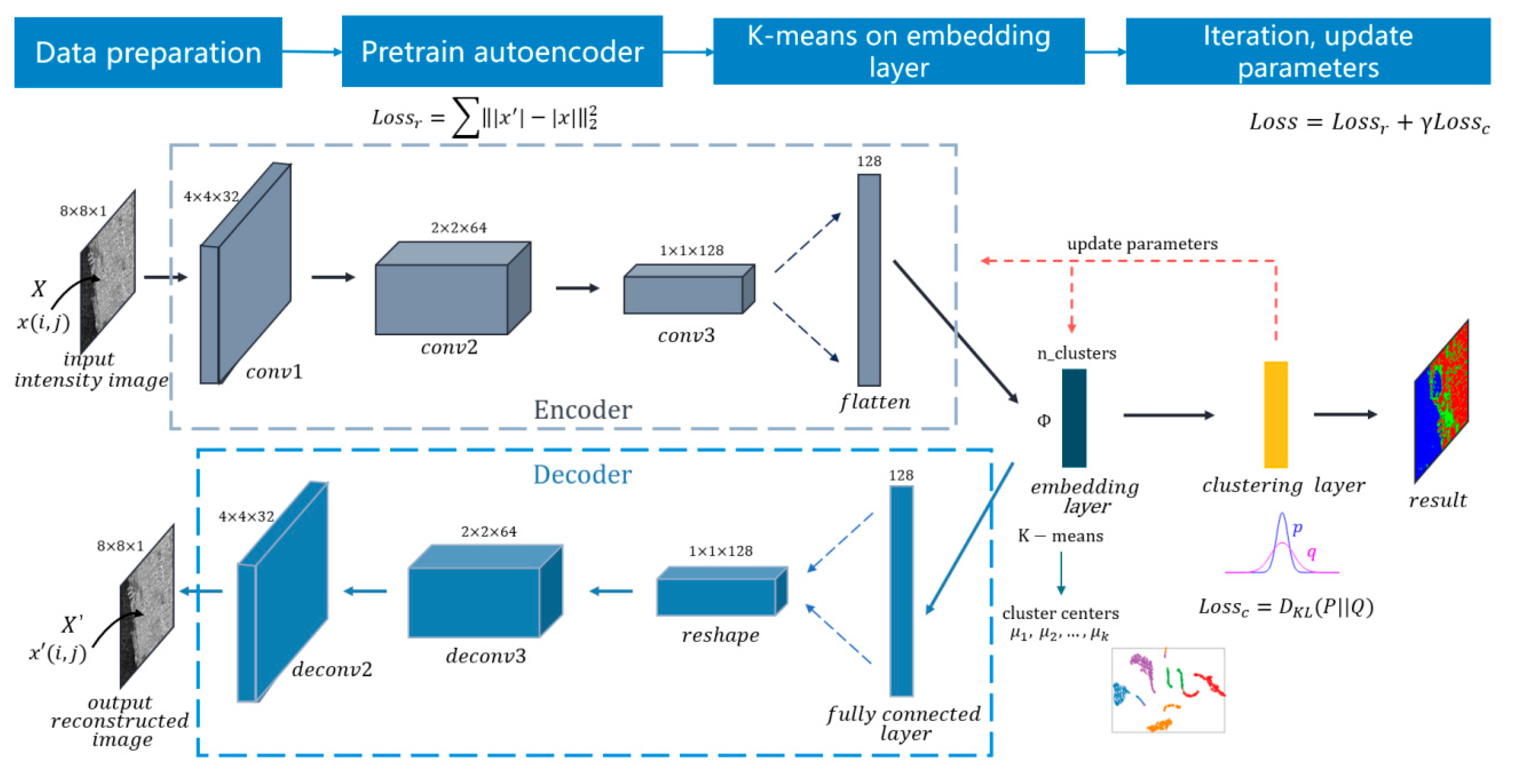
  • We innovatively proposed a complete set of feature extraction, comparison, and analysis method between single-polarized and PolSAR images; in particular, facing the difficulties in unsupervised classification of single-polarized SAR (SP-SAR) images, we adapted the DCEC algorithm to this problem and achieved good clustering.
  • Based on the feature comparison and analysis method, we carried out many experiments, including feature comparison between SP-SAR data and PolSAR data with the same resolution, between HRSP-SAR data and MRPL-SAR data, etc. Based on the results, the characteristics and relationships of different ground types under high resolution and polarimetric situations are summarized, which provides guidance for further applications such as SAR image classification.
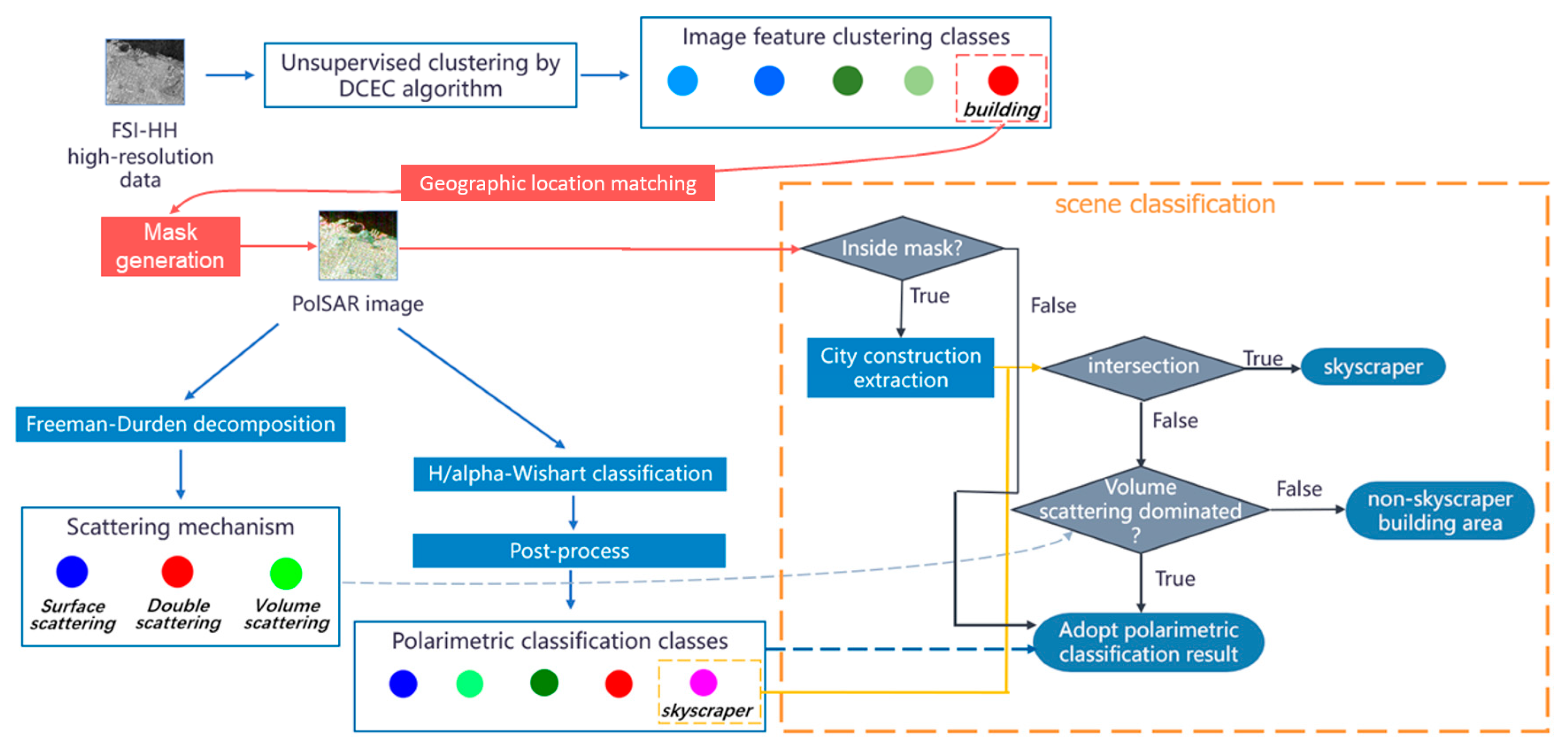
  • An information fusion strategy is proposed, which breaks the boundary of information combination of images of different imaging modes. The strength of HRSP-SAR image feature and PolSAR data physical scattering information are fused for better landcover classification.
The remainder of our paper is organized as follows: Section 2 introduces the feature extraction and comparison method. Section 3 presents our urban area fine-grained classification approach. Experimental results and specific analysis for typical ground targets are given in Section 4, and Section 5 presents conclusions and prospects.

2. Feature Extraction and Comparison Method of High Resolution and Polarimetric SAR Image

2.1. Overview of Comparative Study Method

In this paper, we propose a method to extract, compare and analyze HRSP/MRSP-SAR image domain features and MRPL-SAR physics domain polarimetric features. By using the DCEC algorithm to conduct feature extraction and unsupervised clustering to SP-SAR data, we can get landcover classification with semantic meaning to some extent. Freeman–Durden decomposition and the H/alpha-Wishart classification method are used to analyze PolSAR data. Then, the confusion matrix, mutual information, and scattering plots are used for feature comparison and analysis. Moreover, we summarize the feature relationship and respective strengths of image domain high-resolution information and physics domain polarimetric information, which lead to an effective urban area refined classification method combing their advantages. The whole process of our method is shown in Figure 1.
The following is the step-by-step introduction to the feature extraction, comparison, and evaluation method to single/full-polarized synthetic aperture radar (SAR) data.

2.2. Single-Polarized SAR Image Domain Feature Extraction and Clustering Method

Current research on single-polarized SAR image classification mainly uses deep learning and pattern recognition methods to conduct supervised classification with the combination of labeled samples, while research on unsupervised classification is scarce.
The DCEC algorithm [43] is proposed by Guo et al., integrating the convolutional auto-encoder (CAE) with the K-means clustering algorithm. The advantages of CAE are considering the spatial relationship between pixels and preserving the local structure. It performs remarkably well when tested on the MNIST and USPS datasets. In this paper, the DCEC algorithm is adopted for single-polarized SAR image feature extraction and clustering. The network consists of a CAE and a clustering layer connected to the embedding layer of the CAE. The encoder structure is conv32-conv64-conv128-FC10, the decoder has a mirror-symmetric structure, and the clustering layer has a dimension of the number of clustering categories. The network structure is shown in Figure 2:
DCEC learns the embedded features of CAE and cluster centers simultaneously, and its objective function consists of two parts:
L o s s = L o s s r + γ L o s s c
where L o s s r is the reconstruction loss of CAE, γ is the coefficient to control the distortion of embedding space. L o s s c is the clustering loss, which is defined as the Kullback–Leibler (KL) divergence between target distribution P and soft assignment Q:
L o s s c = D K L ( P | | Q ) = i j p i j log p i j q i j
In (2), q i j is the probability that the embedding point φ i in the embedding layer belongs to the j th class with μ j as the cluster center:
q i j = ( 1 + φ i μ j 2 ) 1 j ( 1 + φ i μ j 2 ) 1 ,
and p i j is defined as:
p i j = q i j 2 / i q i j j ( q i j 2 / i q i j )
The DCEC-based algorithm applied to single-polarized SAR image clustering mainly includes the following steps.
  • Data preprocessing. Filter the image with the appropriate filter size to remove speckle noise, and then normalize and slice the image to adapt to the network input.
  • Pretrain the CAE. Initialize the parameters of CAE to get meaningful target distribution P.
  • Perform the K-means algorithm on the embedding layer of the DCEC network to obtain k initial cluster centers { μ j } j = 1 k corresponding to image embedding features.
  • Let γ = 0.1 and update the CAE network parameters, cluster centers in the embedding layer, and the target distribution P simultaneously through the stochastic gradient descent (SGD) method. Terminate the iteration when the category change between two iterations decreases to a set threshold.
  • Post-processing. Splice the clustered slices and visually display the result, so that we can get the final clustering result.

2.3. PolSAR Image Feature Extraction and Classification Method

Polarimetric decomposition is an important foundation of PolSAR image feature extraction and classification. By practical physical constraints, it identifies the target scattering mechanisms and decomposes the obtained PolSAR data into physical parameters with real significance, which facilitates the interpretation of polarized SAR images. Freeman–Durden decomposition and the H/alpha-Wishart classification method based on Cloude–Pottier decomposition are currently widely used in PolSAR image feature extraction and classification.
Under the scattering symmetry assumption, Freeman–Durden decomposition decomposes the polarimetric coherence matrix T into components corresponding to three scattering mechanisms: surface scattering, double scattering, and volume scattering, which are then used to interpret and analyze the landcover scattering characteristics. Its expression is:
T = f s T S + f d T D + f v T V = f s [ 1 β 0 β | β | 2 0 0 0 0 ] + f d [ | α | 2 α 0 α 1 0 0 0 0 ] + f v [ 2 0 0 0 1 0 0 0 1 ]
where T S , T D , T V are the coherence matrices of surface scattering, double scattering, and volume scattering models respectively, α , β are the model parameters, and f s , f d , f v are weight parameters of the three kinds of scattering components.
Based on eigenvalue decomposition of coherence matrix T, Cloude–Pottier decomposition derived parameters that characterize scattering characteristics of ground targets: scattering entropy (H), anisotropy (A), and average scattering angle (α). Using H and α, a two-dimensional H/alpha plane can be formed. The diagram is shown in Figure 3, and it can distinguish landcover types according to the boundary set by empirical data. It is worth noting that the classification based on the H/alpha plane utilizes the coherency matrix and focuses on the geometric division of scattering characteristics. It is unsupervised and independent of measurement data, which has good robustness and can obtain acceptable results for data under various acquisition conditions.
Wishart distribution can characterize the statistical distribution of PolSAR data. The H/alpha-Wishart method is a combination of the H/alpha classification plane and the Wishart classifier. Based on the maximum likelihood criterion, measure the Wishart distance from pixels to each class center V i and reclassify:
d ( T , V i ) = ln | V i | + t r a c e ( V i 1 T )

2.4. Quantitative Evaluation for Features

In order to compare and analyze the feature characteristics and inter-relationships of SAR data with different imaging modes, we use the confusion matrix and mutual information for quantitative evaluation, and adopt the t-SNE data dimensionality reduction and visualization method to explore the SP-SAR data distribution of different categories in clustering space.

2.4.1. Confusion Matrix and Mutual Information

The confusion matrix is also called the matching matrix, used to measure the consistency of results of two category spaces. We denote the PolSAR classification space and SP-SAR clustering space as x 1 and x 2 , respectively. For polarimetric category i x 1 and SP-SAR clustering category j x 2 , the confusion matrix can be expressed as:
M ( i , j ) = k = 1 N δ ( i , j ) ( x k 1 , x k 2 )
in which
δ ( i , j ) ( x k 1 , x k 2 ) = { 1 x k 1 = i a n d x k 2 = j 0 o t h e r s
Mutual information is a measure of the amount of information that a random variable contains in another. For two random variables X and Y, if their joint probability density function is p ( x , y ) and their boundary probability density functions are p ( x ) and p ( y ) respectively, then their mutual information I ( X ,   Y ) can be defined as the relative entropy between the joint distribution p ( x , y ) and the product distribution p ( x ) p ( y ) :
I ( X , Y ) = x X y Y p ( x , y ) log p ( x , y ) p ( x ) p ( y ) = E p ( x , y ) log p ( X , Y ) p ( X ) p ( Y ) .
For PolSAR data, target information is stored as the polarimetric observation matrix, while for SP-SAR data, target information corresponds to the intensity data. We suppose x 1 and x 2 are PolSAR and SP-SAR class space, respectively. The more information that i x 1 contains about j x 2 (or the more information i x 1 is contained in j x 2 ), the deeper connections between the polarimetric scattering class i and the SP-SAR clustering class j .
Based on the mutual information method, we evaluate the pixel-wise mutual information between two category spaces. And the pixel-based category mutual information between class i and j can be expressed as:
I x 1 x 2 ( i , j ) = log P x 1 x 2 ( i , j ) P x 1 ( i ) P x 2 ( j ) = log P x 1 | x 2 ( i , j ) P x 1 ( i )
where P x 1 x 2 ( i , j ) is the joint distribution of class i and j , P x 1 ( i ) and P x 2 ( j ) is their marginal distribution and P x 1 | x 2 ( i , j ) represents the conditional distribution. In order to calculate (9), we need to get the empirical estimates of P x 1 | x 2 ( i , j ) , P x 1 ( i ) and P x 2 ( j ) , which are represented by the confusion matrix in (7), and accordingly, the empirical estimation of joint distribution and marginal distribution can be defined as:
P ^ x 1 x 2 ( i , j ) = M ( i , j )
P ^ x 1 ( i ) = j M ( i , j )
P ^ x 2 ( j ) = i M ( i , j )
Then, the mutual information matrix I x 1 x 2 ^ ( i , j ) can be empirically estimated. We can see that there exists an overlap between polarimetric class i and SP-SAR clustering class j only when I x 1 x 2 ^ ( i , j ) is non-negative. Hence, I is cut off to 0 for convenience.

2.4.2. t-SNE

In SP-SAR image clustering, the DCEC algorithm mines meaningful image features and clusters iteratively to get the final result, but the discrimination of different categories cannot be reflected. To this end, we adopt the t-SNE algorithm [44] for visible analysis.
The t-SNE algorithm was proposed by Laurens van der Maatens and Geoffrey Hinton, and is mainly used for visualizing and exploring high-dimensional data. It projects the points in the high-dimensional clustering space onto a two-dimensional plane, and obtains low-dimensional data points with good similarity to the original data, keeping similar instances close and separating heterogeneous instances. T-SNE is currently one of the best algorithms in dimensionality reduction and visualization and has been integrated into deep learning algorithm libraries such as sci-kit learn, etc.

3. Refined Classification Method by Information Fusion

PolSAR data contain polarimetric information and can reach a meter-level resolution in current satellite SAR systems. By comparison, the single-polarized mode has higher resolution and can better represent ground details. Based on feature comparison and analysis between data with different imaging modes, we proposed a refined urban area classification method with a combination of both their advantages.
The method extracts the building area by the DCEC-based clustering of HRSP-SAR image and generates its mask on PolSAR image by geographic matching method. Taking account of scattering properties of the masked area, the building area in PolSAR data can be separated. Then, polarimetric unsupervised classification on PolSAR data both inside and outside the mask is conducted, so as to obtain the refined classification in complex areas such as the building area.
The workflow of our proposed method is shown in Figure 4, and detailed steps are described as follows.
  • PolSAR data feature extraction and classification. Analyze the scattering mechanisms by Freeman–Durden decomposition, classify the image using the H/alpha-Wishart classification method, and post-process the result by merging similar or over-segmented categories. Then a classification with clear physical meaning can be obtained.
  • HRSP-SAR data image feature clustering. Cluster the HRSP-SAR data by DCEC method so as to gain city construction extraction.
  • Mask generation on PolSAR image. Based on the building extraction in 2, generate a mask of the corresponding areas on PolSAR data by geographic matching algorithm.
  • Refined classification on PolSAR image. For areas inside the mask, solve the intersection of the masked area in 3 with the high-rise skyscrapers in 1 to extract the skyscrapers. Considering that the HRSP-SAR result may misclassify vegetation as buildings for it is conducted on the intensity information, we refer to the scattering mechanism result by Freeman–Durden decomposition in 1 and employ the polarimetric-based classification result in 1 for masked scenes where volume scattering is dominant, and regard other masked areas as general building areas. And for areas outside the mask, adopt the polarimetric-based classification result in 1.
In this way, we realize the information fusion of images with different imaging modes for better landcover interpretation. Specifically, we integrate the strengths of high-resolution image information (HRII) of FSI data in urban building extraction and edge preservation, as well as the superiority of polarimetric information (PolI) of PolSAR data in natural area analysis, so as to obtain better classification results. It is worth noting that compared with recent work such as [19,37], our work shows some superiority for it needs no labeled samples and has a slight computation burden.

4. Experiments and Results

4.1. Data Description and Experimental Setup

We performed experiments on the C-band Gaofen-3 satellite data of QPSI and FSI imaging modes over the San Francisco area. The detailed information of experimental data is listed in Table 1. We can see that the QPSI mode PolSAR data have polarimetric information, while the FSI mode data have a higher resolution compared with the former. In addition, two sets of data were obtained on 27 March 2019 and 29 April 2020, respectively, which have similar seasonal phase. The optical image and experimental images of the experimental area are displayed in Figure 5.
It is known that the imaging conditions (acquisition time, incidence angle, etc.) of FSI imaging mode data and QPSI imaging mode data are different. However, from the intensity data in Figure 5g,h, we can see that they reflect similar image information, which can both reflect and distinguish buildings, vegetation areas, roads, and water. Moreover, due to the higher resolution, the FSI-HH image contains richer details of ground objects, such as building boundaries and road information.
For PolSAR image, we applied the boxcar filter with a window size of 5 × 5 to remove the speckle noise and maintain image resolution to some level. In the HRSP-SAR clustering experiment, we applied the mean filter with a window size of 3 × 3 to remove noise. Besides, we also performed log-normalization to adapt the image to network input. Considering the combination of neighborhood information and the preservation of image resolution during the patch-based clustering, a patch size of 8 × 8 was used as the network input. In DCEC algorithm, Relu was adopted as the activation function, and the Adam optimization method was used in training, with step size ϵ = 0.001, and exponential decay rate β1 = −0.9, β2 = 0.999. During the cluster center optimization process, the maximum number of iterations is set to 2 × 10 4 , and the iteration process is terminated when category change between two iterations falls below 0.1%. Experiments are conducted on equipment of 64-bit Win10 operating system, with Intel Core i7-9700 [email protected] GHz, NVIDIA GeForce RTX 2080 SUPER, and are run with Python and Matlab 2016.

4.2. Classification Results Based on Image Features and Polarimetric Features

4.2.1. The Case of Three Categories

Perform Freeman–Durden decomposition on PolSAR image and divide the image into three categories: surface scattering (A1), double scattering (A2), and volume scattering (A3). Figure 6 illustrates the polarimetric result. Besides, cluster the single-polarized data into three clusters. The results are shown in Figure 7, and we can see that the three derived categories, a1, a2, and a3, can roughly represent water, building, and vegetation, respectively.

4.2.2. The Case of Five Categories

The classic H/alpha-Wishart algorithm is performed on PolSAR image and the result is shown in Figure 8a. It can be seen that class B3 and B4 both represent skyscrapers, class B2 and class B5 both represent building areas, and class B7 and B8 both represent vegetation areas. In summary, they indicate similar ground targets and exist over-segmentation. Thus, we merge these class pairs and the final classification result is derived in Figure 8b. With reference to the ground truth, we can see that the finally obtained five categories all have clear meanings to some extent. C1~C5 can be interpreted as water, building area, skyscrapers and two kinds of vegetation areas, respectively.
For comparison, we performed the feature extraction and clustering algorithm in 2.2 to various single-polarized SAR data, and clustered each image into five categories, and their results are shown in Figure 9.

4.3. Comparative Study between Image and Physical Feature-Based Classification

4.3.1. Quantitative Analysis

In order to better explore the correlation between different SP-SAR image feature and PolSAR physical scattering mechanism, we calculated the confusion matrices between different DCEC-based clustering results and the polarimetric-based result in the three-class case. Further, mutual information was also worked out. The details of the calculation and strategy of confusion matrices and mutual information were introduced in Section 2.4.1. Table 2, Table 3, Table 4 and Table 5 show the confusion matrices and mutual information matrices between DCEC-based and Freeman–Durden decomposition results, in which Table 5 is calculated using the geographic matching method.
For PolSAR image, the Freeman–Durden decomposition mainly interprets different scattering mechanisms of ground targets; however, the H/alpha-Wishart classification method can further differentiate different ground types.
Moreover, with reference to the ground objects on the optical image, the ground targets are roughly annotated in the experimental area, and they are marked into four categories: water, buildings, skyscrapers, and vegetation. In the annotation process, we regarded various vegetation areas as one category. The ground truth is shown in Figure 10, in which the black region stands for uncertain land-cover class. On this basis, we calculated the mutual information between different DCEC-based SP-SAR results and the ground truth, as well as the mutual information between the polarimetric-based PolSAR classification result with the ground truth in the 5-class case, so as to better analyze and understand the results.
Considering the classification results and the quantitative results in form of mutual information matrices, concrete analysis was as follows:
1.
Result analysis in the case of three classes
From the comparison between different SP-SAR clustering results and the PolSAR Freeman–Durden decomposition result, we can see that all the DCEC-based SP-SAR clustering results in Figure 7 were visually consistent with the polarimetric result (Figure 6) to some extent, showing there exists correlation and indicating that SP image feature has the potential to differentiate ground targets. In addition, in Table 2, Table 3 and Table 4, the diagonal elements gained larger values compared in the same column/row, and the sum of their diagonal values in confusion matrices reached 79.37%, 73.87%, and 75.17%, respectively, which are comparable results with the supervised work to extract physical scattering characteristics by complex-valued CNN in [41]. Table 5 also shows a similar phenomenon. However, its sum value of the confusion matrix diagonal elements was 59.17%, which is relatively lower and was partly because of the differences in acquisition time and incidence angle between the HRSP-SAR and PolSAR data. Quantitative analysis also shows the information inclusion and correlation between image information and polarimetric information.
Further, compared with other clustering results, the HV MRSP-SAR has better performance over surface scattering areas and shows relatively serious misclassification between volume scattering and double scattering areas. One possible explanation is that the intensity of HV channel is relatively lower, in which the built-up areas and the vegetation areas share similar intensity. As a result, it is not obvious enough to reflect landcover texture variation and intensity difference. In addition, the DCEC-based results in Figure 7 divide the upper right mountainous area into two categories, and a large part is red, which is divided into the same category as the urban area. This can also be reflected in Table 2, Table 3, Table 4 and Table 5 that class a2 shows mutual information with volume scattering. We can explain this by the fact that their clustering is intensity-based and the frontal part of mountain areas had strong scattering similar to buildings. By contrast, polarimetric decomposition had a better distinction, indicating that polarimetric information may play an essential role in vegetation extraction.
2.
Result analysis in the case of five classes
Figure 8 and Figure 9 show that: in the 5-class case, both PolSAR classification and DCEC-based SP-SAR clustering can realize the basic distinction of ground targets. Two methods both divide vegetation into two classes (C4, C5 and b4, b5). The difference is that PolSAR classification regards the ocean as one class (C1), and divides the building area into two classes (C2 and C3), being capable of differentiating skyscrapers (C3) from other buildings (C2). By contrast, SP-SAR clustering divides the ocean into two classes (b1 and b2) and divides the building area into one class (b3).
The mutual information in Table 6, Table 7, Table 8 and Table 9 shows some consistency. Class b1 and b2 share mutual information with water, showing the DCEC-based clustering can extract water but over-segment it into two classes. In addition, class b3 shares large mutual information value with building and skyscrapers, which means class b3 and building area contain much information with each other, preliminarily showing the feasibility of extracting buildings through SP image information, even though the distinction between different buildings cannot be realized. Class b4 shares mutual information with both buildings and vegetation area, and this can also be reflected in Figure 9—that there is a poor separation between vegetation and buildings in the SP-SAR clustering result. Additionally, class b5 also shares certain mutual information with vegetation. Four sets of DCEC-based results show that unsupervised clustering on SP-SAR image feature can realize the basic ground targets distinction and obtain classification results with semantic meaning to some extent, and also reflect its effectiveness in building area extraction. Similarly, Table 10 shows that the PolSAR classification can also get a result with semantic meaning: class C1 can indicate water, class C2 and C3 indicate buildings and skyscrapers, respectively, and class C4 and C5 indicates vegetation. In addition, the comparison between Table 10 with the former four shows that polarimetric information may show strength in vegetation and water extraction, as well as distinguishing different buildings. The reason may be that polarimetric information can reflect more physical characteristics of buildings, such as the height and orientation, so as to differentiate different buildings [45,46]. However, the DCEC-based image domain clustering mainly relies on the grayscale information and may have poor performance in strong scattering areas.
Comparing the HRSP-SAR result in Figure 9d and PolSAR result in Figure 8, we can see that though polarimetric information has the above strengths, high-resolution image information (HRII) also has its advantage: it is effective in reflecting details and edges, especially in urban building areas. This indicates that though HRII and polarimetric information (PolI) share some correlation, they are also complementary. Inspired by this, future work can integrate the strengths of FSI high-resolution data in urban building extraction and edge preservation, as well as the superiority of PolSAR data in natural area analysis, so as to obtain better classification results.
Additionally, comparing different MRSP-SAR channels, we can see that co-polarization channels (HH, VV), can better extract the built-up areas. HH channel can better differentiate built-up areas from vegetation areas. This phenomenon can also be reflected in mutual information matrices: that the class b5 only shares mutual information with vegetation in HH MRSP-SAR result in Table 6, however, class b5 also shares mutual information with building in other SP-SAR results (in Table 7, Table 8 and Table 9). In addition, the HV cross-polarization channel is more effective in extracting high-rise built-up areas and water surfaces.

4.3.2. Comparison Analysis on Typical Local Classification Results

Further, we selected several locals for display so as to better analyze and compare characteristics of HRSP-SAR and the MRPL-SAR data. Here, we chose the four areas marked in Figure 7d for display and further comparative analysis: a polo with much vegetation (Zone A), a mixture area of vegetation, roads, and lakes (Zone B), an island with various ground targets (Zone C), and a local typical urban area (Zone D). Their demonstrations are shown in Figure 10, Figure 11, Figure 12 and Figure 13, respectively. Since the FSI HRSP-SAR data used in our experiments are the HH channel, we adopted the result of the HH channel of PolSAR data for comparative analysis.
Zone A corresponds to a polo field, where surface scattering and volume scattering are dominant. It can be seen from Figure 11 that polarimetric method can distinguish different scattering mechanisms and can better distinguish mountain from built-up areas in the upper left of the zone marked by the yellow circle. But PolSAR data have a relatively lower resolution and the filter to remove speckle noise can also bring a reduction in resolution, which may lead to a result that is not ideal in reflection at regional boundaries. By comparison, the DCEC-based FSI HRSP-SAR clustering can better preserve edges and details in the area marked by the yellow box in Figure 11a, which reflects the strength of HRII. However, the clustering is intensity-based, leading to a low degree of separation between built-up areas and mountain areas with similar strong scattering. This is in line with the preceding result analysis.
Zone B is dominated by volume scattering and surface scattering, with a small amount of double scattering. Results in Figure 12 indicate that two sets of SP-SAR clustering results both show similarity to PolSAR result to some degree. There are many small pools with surface scattering characteristics in the area marked by the yellow box in Figure 12a, and can all be reflected in SP-SAR and PolSAR results whether in 3-class or 5-class cases. In addition, due to having a higher resolution, the HRSP-SAR can better retain the pool edges compared with the MRSP-SAR. Moreover, in the case of 5-class, using the results of areas in the yellow circles as an example, the HRSP-SAR clustering shows similar performance to PolSAR in extraction and edge preservation of playgrounds and roads; however, due to a relatively lower resolution, the corresponding MRSP-SAR result is not satisfactory.
Zone C is an island and its optical image is shown in Figure 13a. It can be seen from Figure 13 that two sets of SP-SAR results heavily agree with each other, both having certain effects on ground targets distinction and edge preservation, and also showing certain correlation with polarimetric scattering mechanisms. In the marked yellow circle, the upper part is a built-up area and the lower part contains parking lots and lawns. In the mentioned built-up areas, the HRSP-SAR (Figure 13g) has better performance in building extraction and edge preservation, either compared with the PolSAR (Figure 13c) or the MRSP-SAR (Figure 13e) result. In addition, the areas marked by yellow boxes are mainly buildings around the lawn, which can be reflected in Figure 13g with regular boundaries but cannot be embodied in Figure 13c,e. Through the analysis above, we found that HRII shows some superiority in the extraction and edge preservation of buildings.
Zone D is a part of a typical urban area with high-rise buildings and skyscrapers, and there are roads and vegetation between buildings. Figure 14 shows the feature extraction and classification results of PolSAR and various SP-SAR data. In the 3-class case, various results show some consistency visually and can all realize elementary differentiation among buildings, vegetation, and water. However, in the yellow box marked area in Figure 14a, there is a problem with the PolSAR result (Figure 14b)—the vegetation with volume-scattering characteristics is misclassified as surface scattering. By contrast, this does not appear in SP-SAR clustering results. Furthermore, in the cases of 3-class and 5-class, HRSP-SAR clustering can distinguish the buildings, vegetation, and roads well, with regular boundaries between buildings and roads, and good embodiment of vegetation between buildings. By contrast, the MRPL-SAR and MRSP-SAR results can only partly reflect buildings and vegetation and cannot retain ground details as well as the HRSP-SAR results, which may be partly due to their lower resolution. Thereby we think that HRII has important potential in refined landcover classification. It is worth noting that though the HRSP-SAR clustering can well extract buildings, it cannot distinguish skyscrapers from other buildings as the PolSAR result which can be reflected in the lower left marked area in the yellow circle (Figure 14a) as an instance. This shows the superiority of polarimetric information in differentiating buildings with different scattering properties and also indicates the complementary between HRII and PolI results.

4.3.3. Feature Distribution of Typical Ground Targets

To better understand and analyze the features of different SP-SAR clustering categories and their discrimination, the t-SNE (t-Distributed Stochastic Neighbor Embedding) scatter plot is used to visualize the distribution of data points in high-dimensional feature space. Figure 15 is the dimensionality reduction display of FSI-HH HRSP-SAR data points in the clustering feature space. The scatter plot indicates that on the whole, five categories can distinguish from each other and have desirable discrimination. It should be noted that the results show insufficient division partially between class b3, b4, and b5 (marked in the yellow boxes in Figure 15). The middle box corresponds to class b4 and b5, two classes related to vegetation area; and the left and right boxes correspond to blending of class b3 (related to buildings) with class b4 and b5, respectively, indicating a poor diversion between buildings and vegetation areas. To some extent, this phenomenon is in line with the conclusion obtained from our above analysis, that is, the intensity-based SP-SAR clustering is not good at differentiating buildings from mountain areas for their similar strong scattering intensity.

4.3.4. Summary

In this section, using the presented feature comparison and analysis method, we compare characteristics between different MRSP-SAR and MRPL-SAR data with the same resolution, and between HRSP-SAR and MRPL-SAR data. In addition, we also analyze correlation and complementation on different ground targets between HRII of HRSP-SAR and PolI of MRPL-SAR data, and consequently, the advantages of HRII and PolI for different applications are summarized. Results suggest that it is feasible to mine information of different ground targets from SP-SAR image information. And on a whole, as for ground target interpretation and landcover classification performance, PolI has better capability to distinguish different types of buildings with scattering properties and recognize natural terrains, e.g., distinguish mountain from built-up areas, and prevent over-segmentation in ocean area; by contrast, HRII can better detect buildings from surrounding roads and other scatterers with low backscattering characteristics, showing certain potential in man-made area refined classification. Inspired by this, future work may consider combining the advantage of FSI data with HRII and PolSAR data with PolI, so as to obtain better image classification.

4.4. Urban Area Refined Classification Combing the Advantage of HRII and PolI

It is known that the imaging results of SAR images are susceptible to many factors such as incidence angle and polarization modes. Nevertheless, as can be seen from Figure 5, though FSI and QPSI data have different imaging conditions (such as incidence angle, acquisition time, etc.), the image information of the two is redundant and complementary to a certain extent, which is also analyzed in Section 4.1. In addition, the contours and edges of buildings are relatively stable in a certain period of time. Therefore, though there exist certain differences in imaging conditions, the fusion of HRSP FSI image information is conducive to better interpretation of building information of PolSAR image.
In this section, based on results and conclusions derived from the above experiments, we propose an optimized classification method for urban areas with a combination of the advantage of HRII in extracting built-up areas and the advantage of PolI in extracting natural terrains and differentiating buildings.
Here, we mainly focus on the classification optimization of urban areas with buildings in San Francisco.
In built-up area extraction, we can see that the HRSP-SAR clustering result in Figure 9d shows an obvious advantage over the PolSAR result in Figure 8. Hence, we first extracted built-up areas through DCEC-based HRSP-SAR clustering. Then the mask of extracted built-up area was generated on a PolSAR image by geographic location matching method.
Figure 16a is the built-up area extraction result by HRSP-SAR data. By geographic location matching algorithm, we generated its corresponding mask of the same area on PolSAR data, which is shown in Figure 16b. Results in Figure 16 show that compared with the polarimetric method, using the above method achieved better built-up area extraction performance on PolSAR data. For example, we can identify the vegetation inside built-up areas, as well as the direction and edges of the buildings, which cannot be achieved just in the polarimetric classification result. Next, we conducted polarimetric classification inside and outside the mask. As a result, a refined classification result especially for urban areas was obtained:
Compared with the polarimetric method, the proposed method also requires the unsupervised clustering of FSI image and the geographical matching between the FSI and QPSI data, which may require more computational time. In our experiment, the time used for the two factors mentioned above was 58,357.8 s and 217.5 s, respectively. The proposed method is designed to optimize the classification of urban areas to better extract urban construction. Hence, quantitative analysis mainly focuses on the corresponding region in Figure 16. Based on the ground truth, we quantitatively evaluated the classification performance of urban construction (including general buildings and skyscrapers). Classification accuracy based on the polarimetric method and the proposed method is shown in Table 11.
The result in Figure 17 makes use of PolI advantage in natural terrain interpretation. For example, it can distinguish buildings on the hillside from vegetation in the upper right mountainous area, distinguish skyscrapers from other buildings, and avoid over-segmentation over the ocean. Moreover, our result also considers the HRII advantage, which can better retain the boundaries of buildings and roads. In this way, refined classification in the urban area is realized. In addition, the quantitative results in Table 11 show the proposed method can optimize the classification of urban construction areas, and its overall classification accuracy improved from 50.07% to 63.98%. By applying McNemar’s test with the continuity correction [47] on the results in Table 11, we derived the two-tailed p value less than 0.05, and by conventional criteria, this improvement is considered to be statistically significant. This also proves the superiority and effectiveness of our method.

5. Conclusions

In this paper, we propose a set of feature extraction, comparison, and analysis of image domain information of SP-SAR and polarimetric information of PolSAR data. After using the proposed method to compare the Gaofen-3 data over San Francisco, we found good clustering results of SP-SAR images, reflecting the feasibility of SP-SAR image unsupervised classification, and that gives some reference for tackling the problem of lacking labeled samples as well as lacking empirical theorems and models in SP-SAR classification. In addition, we compared different SP-SAR with PolSAR data with the same resolution, and HRSP-SAR with MRPL-SAR data. We concluded that PolI is better at distinguishing different building areas as well as recognizing natural areas such as water and vegetation; by contrast, HRII has advantages over extracting built-up areas and detecting detailed information such as boundaries and edges. Moreover, based on the feature analysis, we innovatively propose a refined classification method facing urban areas, which combines advantages of both HRII and PolI, breaking through the limitations of existing methods: mainly, supervised work needs labeled samples, or have scarcely combined information of images with different imaging modes. However, the proposed method still has its limitations. In our experiments, only the intensity image information of SP-SAR data was used. In fact, the SP-SAR data are complex-valued that contain more information. Finding ways to extract information beyond the image domain and further explore its application advantages is a meaningful future research direction. In addition, the clustering algorithm plays a significant role in image domain feature processing, and improving the clustering performance with less computational time also needs further exploration.

Author Contributions

Conceptualization, J.Q. and X.Q.; investigation, methodology, J.Q.; validation, J.Q., W.W., X.Q., C.D. and B.L.; writing—original draft preparation, J.Q.; writing—review and editing, X.Q. and Z.W.; project administration, C.D.; funding acquisition, X.Q., C.D. and B.L. All authors have read and agreed to the published version of the manuscript.

Funding

This research was funded by the National Natural Science Foundation of China under Grant Number 61725105 and 62022082.

Institutional Review Board Statement

Not applicable.

Informed Consent Statement

Not applicable.

Data Availability Statement

The experimental data are available from the website of China Ocean Satellite Data Service Center (https://osdds.nsoas.org.cn, accessed on 15 January 2022) after registering and/or ordering.

Acknowledgments

We would like to thank the National Satellite Ocean Application Service for providing the Gaofen-3 SAR data.

Conflicts of Interest

The authors declare no conflict of interest.

References

  1. Huynen, J.R. Theory and applications of the N-target decomposition theorem. Journ. Int. Polarim Rada 1990, 20–22. [Google Scholar]
  2. Krogager, E. New decomposition of the radar target scattering matrix. Electron. Lett. 1990, 26, 1525–1527. [Google Scholar] [CrossRef]
  3. Cloude, S.; Pottier, E. An entropy based classification scheme for land applications of polarimetric SAR. IEEE Trans. Geosci. Remote Sens. 1997, 35, 68–78. [Google Scholar] [CrossRef]
  4. Freeman, A.; Durden, S.L. A three-component scattering model for polarimetric SAR data. IEEE Trans. Geosci. Remote Sens. 1998, 36, 963–973. [Google Scholar] [CrossRef] [Green Version]
  5. Yamaguchi, Y.; Moriyama, T.; Ishido, M.; Yamada, H. Four-component scattering model for polarimetric SAR image decomposition. IEEE Trans. Geosci. Remote Sens. 2005, 43, 1699–1706. [Google Scholar] [CrossRef]
  6. Yamaguchi, Y.; Yajima, Y.; Yamada, H. A Four-Component Decomposition of POLSAR Images Based on the Coherency Matrix. IEEE Geosci. Remote Sens. Lett. 2006, 3, 292–296. [Google Scholar] [CrossRef]
  7. Cloude, S.R. Group Theory and Polarisation Algebra. Optik 1986, 75, 26–36. [Google Scholar]
  8. Wang, Z.; Zeng, Q.; Jiao, J. An Adaptive Decomposition Approach with Dipole Aggregation Model for Polarimetric SAR Data. Remote Sens. 2021, 13, 2583. [Google Scholar] [CrossRef]
  9. Ainsworth, T.L.; Wang, Y.; Lee, J.-S. Model-Based Polarimetric SAR Decomposition: An L 1 Regularization Approach. IEEE Trans. Geosci. Remote Sens. 2021, 60, 1–13. [Google Scholar] [CrossRef]
  10. Singh, G.; Yamaguchi, Y. Model-Based Six-Component Scattering Matrix Power Decomposition. IEEE Trans. Geosci. Remote Sens. 2018, 56, 5687–5704. [Google Scholar] [CrossRef]
  11. Singh, G.; Malik, R.; Mohanty, S.; Rathore, V.; Yamada, K.; Umemura, M.; Yamaguchi, Y. Seven-Component Scattering Power Decomposition of POLSAR Coherency Matrix. IEEE Trans. Geosci. Remote Sens. 2019, 57, 8371–8382. [Google Scholar] [CrossRef]
  12. Van Zyl, J.J. Unsupervised classification of scattering behavior using radar polarimetry data. IEEE Trans. Geosci. Remote Sens. 1989, 27, 36–45. [Google Scholar] [CrossRef]
  13. Cloude, S.R. An entropy based classification scheme for polarimetric SAR data. In Proceedings of the Geoscience and Remote Sensing Symposium, IGARSS ‘95. ‘Quantitative Remote Sensing for Science and Applications’, Firenze, Italy, 10–14 July 1995. [Google Scholar]
  14. Lee, J.-S.; Grunes, M.; Ainsworth, T.; Du, L.-J.; Schuler, D.; Cloude, S. Unsupervised classification using polarimetric decomposition and the complex Wishart classifier. IEEE Trans. Geosci. Remote Sens. 1999, 37, 2249–2258. [Google Scholar] [CrossRef]
  15. Cao, F.; Hong, W.; Wu, Y.; Pottier, E. An Unsupervised Segmentation With an Adaptive Number of Clusters Using the SPAN/H/α/A Space and the Complex Wishart Clustering for Fully Polarimetric SAR Data Analysis. IEEE Trans. Geosci. Remote Sens. 2007, 45, 3454–3467. [Google Scholar] [CrossRef]
  16. Lee, J.-S.; Grunes, M.; Pottier, E.; Ferro-Famil, L. Unsupervised terrain classification preserving polarimetric scattering characteristics. IEEE Trans. Geosci. Remote Sens. 2004, 42, 722–731. [Google Scholar] [CrossRef]
  17. Ratha, D.; Bhattacharya, A.; Frery, A.C. Unsupervised Classification of PolSAR Data Using a Scattering Similarity Measure Derived From a Geodesic Distance. IEEE Geosci. Remote Sens. Lett. 2017, 15, 151–155. [Google Scholar] [CrossRef] [Green Version]
  18. Qu, J.; Qiu, X.; Ding, C.; Lei, B. Unsupervised Classification of Polarimetric SAR Image Based on Geodesic Distance and Non-Gaussian Distribution Feature. Sensors 2021, 21, 1317. [Google Scholar] [CrossRef]
  19. Liu, C.; Li, H.-C.; Liao, W.; Philips, W.; Emery, W.J. Variational Textured Dirichlet Process Mixture Model With Pairwise Constraint for Unsupervised Classification of Polarimetric SAR Images. IEEE Trans. Image Process. 2019, 28, 4145–4160. [Google Scholar] [CrossRef]
  20. Zhu, J.H.; Guo, H.D.; Fan, X.T.; Zhu, B.Q. The Application of the Wavelet Texture Method to the Classification of Single-band, Single-polarized and High-resolution SAR Images. Remote Sens. Land Resour. 2005, 63, 36–39. [Google Scholar] [CrossRef]
  21. Hu, D.; Li, J.; Chen, Y.; Jiang, W. Water and Settlement Area Extraction from Single-band Single-polarization SAR Images Based on SVM Method. J. Image Graph. 2008, 13, 257–263. [Google Scholar]
  22. Wu, C. Land Coverage Classification Based on Spatial and Radiation Characteristics in HR SAR Image and System Design. Master’s Thesis, Shanghai Jiao Tong University, Shanghai, China, 2012. [Google Scholar]
  23. Chamundeeswari, V.; Singh, D.; Singh, K. Unsupervised land cover classification of SAR images by contour tracing. In Proceedings of the 2007 IEEE International Geoscience and Remote Sensing Symposium, Barcelona, Spain, 23–28 July 2007; pp. 547–550. [Google Scholar]
  24. Chamundeeswari, V.V.; Singh, D.; Singh, K. An Analysis of Texture Measures in PCA-Based Unsupervised Classification of SAR Images. IEEE Geosci. Remote Sens. Lett. 2009, 6, 214–218. [Google Scholar] [CrossRef]
  25. Esch, T.; Schenk, A.; Thiel, M.; Ullmann, T.; Schmidt, M.; Dech, S. Land cover classification based on single-polarized VHR SAR images using texture information derived via speckle analysis. In Proceedings of the 2010 IEEE International Geoscience and Remote Sensing Symposium, Honolulu, HI, USA, 25–30 July 2010; pp. 1875–1878. [Google Scholar]
  26. Available online: http://sw.chreos.org/challenge (accessed on 16 January 2022).
  27. Zhao, Z.; Jiao, L.; Zhao, J.; Gu, J.; Zhao, J. Discriminant deep belief network for high-resolution SAR image classification. Pattern Recognit. 2017, 61, 686–701. [Google Scholar] [CrossRef]
  28. Duan, Y.; Tao, X.; Han, C.; Qin, X.; Lu, J. Multi-Scale Convolutional Neural Network for SAR Image Semantic Segmentation. In Proceedings of the 2018 IEEE Global Communications Conference (GLOBECOM), Abu Dhabi, United Arab Emirates, 9–13 December 2018; pp. 1–6. [Google Scholar]
  29. Geng, J.; Fan, J.; Wang, H.; Ma, X.; Li, B.; Chen, F. High-Resolution SAR Image Classification via Deep Convolutional Autoencoders. IEEE Geosci. Remote Sens. Lett. 2015, 12, 2351–2355. [Google Scholar] [CrossRef]
  30. Zhou, Y.; Wang, H.; Xu, F.; Jin, Y.-Q. Polarimetric SAR Image Classification Using Deep Convolutional Neural Networks. IEEE Geosci. Remote Sens. Lett. 2016, 13, 1935–1939. [Google Scholar] [CrossRef]
  31. Wang, H.; Xu, F.; Jin, Y.-Q. A Review of Polsar Image Classification: From Polarimetry to Deep Learning. In Proceedings of the IGARSS 2019-2019 IEEE International Geoscience and Remote Sensing Symposium, Yokohama, Japan, 28 July–2 August 2019; pp. 3189–3192. [Google Scholar]
  32. Xie, W.; Jiao, L.; Hou, B.; Ma, W.; Zhao, J.; Zhang, S.; Liu, F. POLSAR Image Classification via Wishart-AE Model or Wishart-CAE Model. IEEE J. Sel. Top. Appl. Earth Obs. Remote Sens. 2017, 10, 3604–3615. [Google Scholar] [CrossRef]
  33. Chen, Y.; Jiao, L.; Li, Y.; Zhao, J. Multilayer Projective Dictionary Pair Learning and Sparse Autoencoder for PolSAR Image Classification. IEEE Trans. Geosci. Remote Sens. 2017, 55, 6683–6694. [Google Scholar] [CrossRef]
  34. Lv, Q.; Dou, Y.; Niu, X.; Xu, J.; Xu, J.; Xia, F. Urban land use and land cover classification using remotely sensed SAR data through deep beliefnetworks. J. Sens. 2015, 2015, 538063. [Google Scholar] [CrossRef] [Green Version]
  35. Zhang, Z.; Wang, H.; Xu, F.; Jin, Y.-Q. Complex-Valued Convolutional Neural Network and Its Application in Polarimetric SAR Image Classification. IEEE Trans. Geosci. Remote Sens. 2017, 55, 7177–7188. [Google Scholar] [CrossRef]
  36. Zhao, J.; Guo, W.; Liu, B.; Zhang, Z.; Yu, W.; Cui, S. Preliminary exploration of SAR image land cover classification with noisy labels. In Proceedings of the 2017 IEEE International Geoscience and Remote Sensing Symposium (IGARSS), Fort Worth, TX, USA, 23–28 July 2017; pp. 3274–3277. [Google Scholar]
  37. Ahishali, M.; Kiranyaz, S.; Ince, T.; Gabbouj, M. Classification of polarimetric SAR images using compact convolutional neural networks. GISci. Remote Sens. 2021, 58, 28–47. [Google Scholar] [CrossRef]
  38. Song, Q.; Xu, F.; Jin, Y.Q. Radar Image Colorization: Converting Single-Polarization to Fully Polarimetric Using Deep Neural Networks. IEEE Access 2017, 6, 1647–1661. [Google Scholar] [CrossRef]
  39. Zhang, J.; Qiu, X.; Wang, X.; Jin, Y. Full-polarimetric scattering characteristics prediction from single/dual-polarimetric SAR data using convolutional neural networks. J. Eng. 2019, 7459–7463. [Google Scholar] [CrossRef]
  40. Zhao, J.; Datcu, M.; Zhang, Z.; Xiong, H.; Yu, W. Contrastive-Regulated CNN in the Complex Domain: A Method to Learn Physical Scattering Signatures From Flexible PolSAR Images. IEEE Trans. Geosci. Remote Sens. 2019, 57, 10116–10135. [Google Scholar] [CrossRef]
  41. Huang, Z.; Datcu, M.; Pan, Z.; Qiu, X.; Lei, B. HDEC-TFA: An Unsupervised Learning Approach for Discovering Physical Scattering Properties of Single-Polarized SAR Image. IEEE Trans. Geosci. Remote Sens. 2021, 59, 3054–3071. [Google Scholar] [CrossRef]
  42. Qu, J.; Qiu, X.; Ding, C. A Study of Recovering Polsar Information from Single-Polarized Data Using DNN. In Proceedings of the 2021 IEEE International Geoscience and Remote Sensing Symposium IGARSS, Brussels, Belgium, 11–16 July 2021. [Google Scholar] [CrossRef]
  43. Guo, X.; Liu, X.; Zhu, E.; Yin, J. Deep Clustering with Convolutional Autoencoders. In Post-Quantum Cryptography; Springer Science and Business Media LLC: Cham, Switzerland, 2017; pp. 373–382. [Google Scholar]
  44. Van der Maaten, L.; Hinton, G. Visualizing Data Using t-SNE. J. Mach. Learn. Res. 2008, 9, 2579–2605. [Google Scholar]
  45. Lee, J.S.; Krogager, E.; Ainsworth, T.L.; Boerner, W.M. Polarimetric Analysis of Radar Signature of a Manmade Structure. IEEE Geosci. Remote Sens. Lett. 2006, 3, 555–559. [Google Scholar] [CrossRef]
  46. Franceschetti, G.; Iodice, A.; Riccio, D. A canonical problem in electromagnetic backscattering from buildings. IEEE Trans. Geosci. Remote Sens. 2002, 40, 1787–1801. [Google Scholar] [CrossRef]
  47. Edwards, A.L. Note on the “correction for continuity” in testing the significance of the difference between correlated proportions. Psychometrika 1948, 13, 185–187. [Google Scholar] [CrossRef]
Figure 1. The diagram of the proposed method.
Remotesensing 14 01412 g001
Figure 2. Deep Convolutional Embedding Clustering (DCEC) network structure and algorithm flowchart.
Remotesensing 14 01412 g002
Figure 3. H/alpha classification plane.
Remotesensing 14 01412 g003
Figure 4. Workflow of the proposed refined classification method.
Remotesensing 14 01412 g004
Figure 5. Presentation of experimental data. (a) is the optical image of experimental area, (b) is FSI-HH HRSP-SAR intensity image, (ce) represent the HH, HV, VV single-polarized channel of medium-resolution PolSAR (MRPL-SAR) intensity image, respectively, (f) is the Pauli pseudo-image of MRPL-SAR data, (g,h) are enlarged displays of the marked area in (b,c) in turn, and it can be seen that the FSI-HH image can better reflect the detailed ground texture due to its higher resolution.
Remotesensing 14 01412 g005aRemotesensing 14 01412 g005b
Figure 6. Freeman–Durden decomposition result of PolSAR image.
Remotesensing 14 01412 g006
Figure 7. Clustering results of different single-polarized SAR images in the case of three classes. (ac) are clustering results of HH, HV, VV single-polarized channel of PolSAR data, respectively, (d) is the clustering result of FSI-HH HRSP-SAR image, and (e) is the color set.
Remotesensing 14 01412 g007aRemotesensing 14 01412 g007b
Figure 8. PolSAR image classification result. (a) Classification result by H/alpha-Wishart algorithm. (b) Final polarimetric classification after post-processing.
Remotesensing 14 01412 g008
Figure 9. Clustering results of different single-polarized SAR images in the case of five classes. (ac) are clustering results of HH, HV, VV single-polarized channel of PolSAR data, respectively, (d) is the clustering result of FSI-HH HRSP-SAR image, and (e) is the color set.
Remotesensing 14 01412 g009aRemotesensing 14 01412 g009b
Figure 10. Ground truth of the experimental area.
Remotesensing 14 01412 g010
Figure 11. Enlarged results of Zone A. (a) is the optical image, (b) is the Freeman–Durden decomposition result of PolSAR image, (c) is the polarimetric classification result of PolSAR image, (d,e) are the clustering results of HH MRSP-SAR data in the case of three and five categories, respectively, (f,g) are the clustering results of FSI-HH HRSP-SAR data in the case of three and five classes.
Remotesensing 14 01412 g011aRemotesensing 14 01412 g011b
Figure 12. Enlarged results of Zone B. (a) is the optical image, (b) is the Freeman–Durden decomposition result of PolSAR image, (c) is the polarimetric classification result of PolSAR image, (d,e) are the clustering results of HH MRSP-SAR data in the case of three and five categories, respectively, (f,g) are the clustering results of FSI-HH HRSP-SAR data in the case of three and five classes.
Remotesensing 14 01412 g012aRemotesensing 14 01412 g012b
Figure 13. Enlarged results of Zone C. (a) is the optical image, (b) is the Freeman–Durden decomposition result of PolSAR image, (c) is the polarimetric classification result of PolSAR image, (d,e) are the clustering results of HH MRSP-SAR data in the case of three and five categories, respectively, (f,g) are the clustering results of FSI-HH HRSP-SAR data in the case of three and five classes.
Remotesensing 14 01412 g013aRemotesensing 14 01412 g013b
Figure 14. Enlarged results of Zone D. (a) is the optical image, (b) is the Freeman–Durden decomposition result of PolSAR image, (c) is the polarimetric classification result of PolSAR image, (d,e) are the clustering results of HH MRSP-SAR data in the case of three and five categories, respectively, (f,g) are the clustering results of FSI-HH HRSP-SAR data in the case of three and five classes.
Remotesensing 14 01412 g014aRemotesensing 14 01412 g014b
Figure 15. T-SNE scatter plot of FSI-HH HRSP-SAR data points in clustering feature space.
Remotesensing 14 01412 g015
Figure 16. Built-up area extraction. (a) is the extraction result on HRSP-SAR data, and (b) is the built-up area mask generated on PolSAR data.
Remotesensing 14 01412 g016aRemotesensing 14 01412 g016b
Figure 17. Refined classification result.
Remotesensing 14 01412 g017
Table 1. Experimental data description.
Imaging ModeQPSIFSI
PolarizationFull polarization
(HH, HV, VH, VV)
Dual polarization
(HH, HV)
Acquisition Data27 March 201929 April 2020
Pixel spacing-rg (m)2.242.24
Pixel spacing-az (m)5.293.07
Incidence angle (°)36.24 (central)47.75 (central)
DirectionDECDEC
Table 2. Confusion matrix and mutual information matrix between HH medium resolution single-polarized SAR (MRSP-SAR) clustering and PolSAR Freeman–Durden decomposition result.
MRSP-SAR Classa1a2a3a1a2a3
PolSAR Class Confusion Matrix (%)Mutual Information Matrix
A142.6015.790.279900
A20.2719.812.1400.47580
A32.41916.9700.21130.3805
Table 3. Confusion matrix and mutual information matrix between HV MRSP-SAR clustering and PolSAR Freeman–Durden decomposition result.
MRSP-SAR Classa1a2a3a1a2a3
PolSAR Class Confusion Matrix (%)Mutual Information Matrix
A143.980.4250.287100
A20.3917.853.9800.38620
A31.614.7412.0400.49910.3050
Table 4. Confusion matrix and mutual information matrix between VV MRSP-SAR clustering and PolSAR Freeman–Durden decomposition result.
MRSP-SAR Classa1a2a3a1a2a3
PolSAR Class Confusion Matrix (%)Mutual Information Matrix
A141.430.897.080.269600
A20.4318.053.7300.45630
A33.229.4815.6900.20700.3192
Table 5. Confusion matrix and mutual information matrix between FSI-HH HRSP-SAR clustering and PolSAR Freeman–Durden decomposition result.
HRSP-SAR Classa1a2a3a1a2a3
PolSAR Class Confusion Matrix (%)Mutual Information Matrix
A137.954.308.080.177300
A24.4110.946.6200.30150
A37.779.6310.3000.24390.1724
Table 6. Confusion matrix and mutual information matrix between HH MRSP-SAR result and the ground truth.
MRSP-SARb1b2b3b4b5
GT Class Confusion Matrix (%)
Water19.2037.730.050.230.80
Building0010.145.451.83
Skyscraper001.950.970.24
Vegetation0.780.012.615.9812.02
Mutual Information Matrix
Water0.21910.2363000
Building000.59610.39380
Skyscraper000.62130.38660
Vegetation0000.34500.5765
Table 7. Confusion matrix and mutual information matrix between HV MRSP-SAR result and the ground truth.
MRSP-SARb1b2b3b4b5
GT Class Confusion Matrix (%)
Water32.0724.8700.011.06
Building006.747.772.91
Skyscraper002.510.550.11
Vegetation00.032.579.409.39
Mutual Information Matrix
Water0.23640.2359000
Building000.51470.40060.0939
Skyscraper000.826300
Vegetation000.00680.39430.5129
Table 8. Confusion matrix and mutual information matrix between VV MRSP-SAR result and the ground truth.
MRSP-SARb1b2b3b4b5
GT Class Confusion Matrix (%)
Water24.4430.980.060.971.57
Building0.01011.433.332.65
Skyscraper002.470.450.25
Vegetation1.060.115.355.509.38
Mutual Information Matrix
Water0.21790.2349000
Building000.53130.27040.0416
Skyscraper000.60620.14420
Vegetation000.11260.39930.5004
Table 9. Confusion matrix and mutual information matrix between FSI-HH HRSP-SAR result and the ground truth.
HRSP-SARb1b2b3b4b5
GT Class CONFUSION matrix(%)
Water24.4031.010.010.034.61
Building0011.014.963.56
Skyscraper001.800.570.38
Vegetation0.060.243.895.657.81
Mutual Information Matrix
Water0.22030.2181000
Building000.52790.35500.0468
Skyscraper000.59260.26730
Vegetation000.12040.45530.4321
Table 10. Confusion matrix and mutual information matrix between PolSAR result and the ground truth.
PolarimetricC1C2C3C4C5
GT Class Confusion Matrix (%)
Water55.510.0300.082.38
Building08.861.266.700.60
Skyscraper01.121.440.530.07
Vegetation0.030.910.0910.2510.13
Mutual Information Matrix
Water0.23640000
Building00.66810.41330.34040
Skyscraper00.51111.212100
Vegetation0000.43540.5550
Table 11. Classification accuracy (%) of urban construction by polarimetric method and the proposed method.
BuildingsSkyscrapersOverall
Polarimetric method51.0945.6550.07
Proposed method68.1945.6563.98
Publisher’s Note: MDPI stays neutral with regard to jurisdictional claims in published maps and institutional affiliations.

