Article

Improved IDW Interpolation Application Using 3D Search Neighborhoods: Borehole Data-Based Seismic Liquefaction Hazard Assessment and Mapping

1
Department of Geotechnical Engineering Research, Korea Institute of Civil Engineering and Building Technology, Goyang-si 10223, Gyeonggi-do, Republic of Korea
2
Department of Professional Service, MOSAIC TAILOR Incorporated, Suwon-si 16514, Gyeonggi-do, Republic of Korea
*
Author to whom correspondence should be addressed.
Appl. Sci. 2022, 12(22), 11652; https://doi.org/10.3390/app122211652
Submission received: 13 October 2022 / Revised: 11 November 2022 / Accepted: 15 November 2022 / Published: 16 November 2022
(This article belongs to the Section Civil Engineering)

Abstract

:

Featured Application

There are 3 applications used in this study. (1) Esri’s ArcGIS is used for modeling/visualization geo-spatial data and publishing 3D web mapping application; (2) MathWorks’s MATLAB is used for borehole data preprocessing and liquefaction hazard assessment; (3) Robert McNeel & Associates’s Rhino/Grasshopper is used for developing improved IDW algorithm.

Abstract

Traditional inverse distance weighting (IDW) interpolation is a process employed to estimate unknown values based on neighborhoods in 2D space. Proposed in this study is an improved IDW interpolation method that uses 3D search neighborhoods for effective interpolation on vertically connected observation data, such as water level, depth, and altitude. Borehole data are the data collected by subsurface boring activities and exhibit heterogeneous spatial distribution as they are densely populated near civil engineering or construction sites. In addition, they are 3D spatial data that show different subsurface characteristics by depth. The subsurface characteristics observed as such are used as core data in spatial modeling in fields, such as geology modeling, estimation of groundwater table distribution, global warming assessment, and seismic liquefaction assessment, among others. Therefore, this study proposed a seismic liquefaction assessment and mapping workflow using an improved IDW application by combining geographic information system (GIS) (ArcGIS (Esri, Redlands, CA, USA)), NURBS-based 3D CAD system (Rhino/Grasshopper (Robert McNeel & Associates, Seattle, WA, USA)), and numerical analysis system (MATLAB (MathWorks, Natick, MA, USA)). The 3D neighborhood search was conducted by the B-rep-based 3D topology analysis, and the mapping was done under the 2.5D environment by combining the voxel layer, DEM, and aerial images. The experiment was performed by collecting data in Songpa-gu, Seoul, which has the highest population density among the OECD countries. The results of the experiment showed between 7 and 105 areas with liquefaction potentials according to the search distance and the method of the approach. Finally, this study improved users’ accessibility to interpolation results by producing a 3D web app that used REST API based on OGC I3S Standards. Such an approach can be applied effectively in spatial modeling that uses 3D observation data, and in the future, it can contribute to the expansion of 3D GIS application.

1. Introduction

1.1. Background

Spatial interpolation is a technique that estimates an unknown value in a location not sampled from spatiotemporally distributed known values. It is widely used as a raster-based spatial analysis in topographic modeling [1], fine dust assessment [2], climate modeling [3], landslide risk assessment [4], and even medical image analysis [5]. The estimation of an unknown value in interpolation is determined by the spatial relationship, which can be defined differently by the neighborhood search method. In the case of a square-based grid, the neighborhoods are typically Rook, Bishop, and Queen that determine four or eight neighboring cells, and to minimize the edge effect of the square grid, a hexagon grid can be used (Figure 1) [6,7]. However, such traditional raster-based neighborhood analysis is performed based on the assumption of a 2D vector space and is limitedly applied to observation data distributed in 3D space (i.e., fine dust assessment by altitude using a drone [8], borehole-based geology modeling [9], marine environment assessment [10]). As such, the data observed in the spatial context, such as water level, depth, or altitude, exhibit both horizontal and vertical connectivity. Thus, a neighborhoods search during interpolation also needs to be performed in 3D space, and a more realistic spatial modeling can be possible via 3D interpolation. Therefore, this study proposed an improved interpolation method using 3D search neighborhoods and attempted to examine the results by applying them to actual cases.

1.2. Literature Review

1.2.1. Borehole Data

The borehole data collected from boring activities are managed by the boring coordinates, ground level and depth, geological information by depth, and site test results (standard penetration test). In other words, the boring coordinates represent a horizontal position and using the relative height between depth and ground level, a vertical position of the borehole location can be determined. The processed borehole data becomes 3D spatial data that can browse geological information by depth. Such georeferenced borehole data can be utilized in various spatial modeling, such as geology modeling [11], estimation of groundwater table distribution [12], global warming assessment [13], seismic liquefaction assessment [14], among others. However, due to the characteristics of the boring environment, subsurface boring results show a heterogeneous spatial arrangement where they are distributed linearly near the roads or are densely populated near housing sites, as opposed to general observation data that are randomly distributed. Therefore, they are limited in the application of geostatistical spatial interpolation to which spatial arrangement is important. Furthermore, since individual boreholes are composed of 3D coordinates, general 2D interpolation methods are limited in completely reflecting the characteristics of borehole data that are densely distributed in a vertical direction of the ground surface.

1.2.2. Spatial Interpolation Methods

Spatial interpolation can be categorized into point interpolation and areal interpolation [15]. While both methods are identical in that they both estimate unknown values on a location that is not sampled from spatiotemporally distributed observation data, they are used in completely different geographical problems [16]. Generally, areal interpolation uses simple areal weighting [17] or dasymetric mapping [18], and these are applied to reassign the spatial unit of the observed data [19]. On the other hand, the point interpolation can be further categorized into local neighborhood approach-based interpolation (i.e., IDW, Natural neighbor interpolation, TIN), geostatistical approach-based interpolation (i.e., Kriging), and variational approach-based interpolation (i.e., Spline), and as has been discussed, it can often perform spatial modeling through the estimation of an unknown value or resample the raster data resolution [20]. Since the aim of this study is the interpolation of 3D point data distributed in 3D space, the literature on areal interpolation is not reviewed additionally.
The point interpolation that is most widely used in geographical information systems (GIS) these days applies to inverse distance weighting (IDW) and Kriging. By characteristics, there exist improved models of these methods (i.e., Multivariate blended IDW surfaces and volumes [20,21,22,23], Co-Kriging [24], Empirical Bayesian Kriging [25,26], but these are basically identical in that the closer the distance between a cell with an unknown value and neighborhoods with known values, the stronger the correlation that is assumed. The biggest difference between IDW and Kriging is that Kriging is a probabilistic interpolation method that determines the weighting value based not only on distance but on spatial autocorrelation toward observed data, and it produces an interpolation function based on a covariance or variogram model [27]. Due to such characteristics, it is effective in fields with a spatial arrangement from a geostatistical perspective, such as mining and petroleum, geochemistry, geology, and ecology [20]. In addition, as a new approach for voxel data processing and visualization in recent years, 3D search neighborhoods-based 3D Empirical Bayesian Kriging is being applied to GIS applications [28].
On the other hand, IDW is a deterministic interpolation method that determines weight based on the distance between neighborhoods and a location with unknown values and estimates unknown values by assigning the weighting value to neighboring observation data. As such, IDW has a simple basic assumption and offers efficient processing, but its disadvantage is that it generates local extrema on the estimation surface (Figure 2). Due to such characteristics, IDW is limited in topographic modeling that reproduces natural (or smooth) local shapes, rather than the quantitative evaluation of the interpolation predictive capabilities.
These traditional interpolation methods could not satisfy the requirements that should be considered in 3D space since they were developed assuming 2D spatial modeling. Thus, many scholars suggested an improved method related to traditional interpolation in terms of 3D search neighbors and an interpolation function. When considering the interpolation method, Yang et al. proposed a Kriging approach based on a divide-and-conquer strategy through linear combination on multiple prediction results to improve the classical Co-Kriging method where all the input data are fitted at once [29]. Moreover, Car et al. proposed an effective method to recreate uniform meshes from point cloud data through improved interpolation based on the Radial Basis Function (RBF) [30], and it is similar to Dual Kriging [27]. These 3D interpolation methods provide modeling results that more concern the real world but have limits on reflecting the borehole data that have a vertically dense distribution. In 2D GIS, the search area is generalized to a circle, and the search distance to a radius. Yet, for vertically concentrated data, such as borehole data, searching neighbors by using an asymmetrical distance in a 3D space is more desirable than to search a neighbor by using the same distance for every direction. 3D search neighborhoods improvement is important in the spatial interpolation method since the outcome may greatly vary depending on the approach determining the neighbors though the interpolation function is the same. In terms of 3D search neighborhoods, Liu et al. proposed 3D search neighborhoods based on a constrained Delaunay triangulation and the large scaled 3D geological modeling method based on borehole data using IDW interpolation (Figure 3a) [31].
And Sun et al. proposed an improved IDW in which they created a bounding box in vertical and horizontal directions, which is indexed from the location with unknown values, and used it in the neighborhood search for interpolation (Figure 3b) [9]. an approach was used in separating and running the neighborhood search distance horizontally and vertically, and is advantageous in effectively reflecting the characteristics of borehole data that are densely populated vertically. However, neighborhood search by using Delaunay triangle has limitation on explicit search distance limits. In addition, horizontal/vertical bounding box-based approach that converts the Rook that searches neighbors perpendicular to the XY axis into the XY and XZ axes, and thus, it is limited in searching neighborhoods located diagonally.
In order to alleviate the problems, this study proposed an improved IDW algorithm to which fine spheroid-based 3D search neighborhoods is applied, which can search all directional neighborhoods. This approach can maintain the accuracy of IDW interpolation, which is the most actively used in 3D geological modeling and can efficiently expand the traditional search neighborhood method to a 3D environment. Finally, proposed IDW results were examined by performing the seismic liquefaction assessment and mapping.

2. Research Method

2.1. Preprocessing of Experiment Data

The coordinates of borehole data sometimes are recorded in different coordinate systems by period. If no coordinate system is clearly described during the recording, data can be unified into a correct coordinate system using georeferencing based on aerial image data under a well-known coordinate system. In addition, if coordinates have been recorded based on a geographic coordinate system, they are converted by a projected coordinate system to intuitively notate the unit of the neighborhood search scope.
Height and depth are important information in determining the 3D location coordinates of borehole data. As boring is surveyed for a long period, the recorded height can be shown differently from the current height, and the accuracy of the measurement may also vary by the worker who measured it. Thus, as the experiment data, the height data generated from the precise DEM that can reflect reality are used [32]. While the relative height from the height toward the subsurface is recorded as depth, it can sometimes be recorded in a negative or positive value. Therefore, the absolute value of the recorded depth was first taken and then, using the height calculated above, the 3D location coordinates of borehole data are ultimately determined.

2.2. Seismic Liquefaction Assessment

Seismic liquefaction means a phenomenon in which a stable ground structure loses stability and behaves similar to water during an earthquake or other seismic events. The factor of safety against liquefaction ( F L ) can be assessed by dividing the resistance of the foundation against liquefaction (cyclic resistance ratio; CRR) by the external force to the subsurface due to earthquake (cyclic shear stress ratio; CSR) based on the subsurface information acquired from borehole data. As such, this study produced CSR in depth by performing the 1D equivalent linear method and CRR by the Common Applications of the Seismic Design Code by the Ministry of Land, Infrastructure, and Transport, and the Structural Foundation Design Standards by Korea Geotechnical Society [33] (Equations (1) and (2))
C R R = τ ι σ υ 7.5 = 1 34 N 1 60 , c s + N 1 60 , c s 135 + 50 10 · N 1 60 , c s + 45 2 1 200
C S R = τ m a x d σ υ = 0.65 α m a x d g σ v σ υ
where
N 1 60 , c s : N value that compensated the overburden load, energy efficiency of 60%, and fine content;
σ υ : Overburden pressure under the depth at which liquefaction is to be assessed;
σ v : Effective overburden pressure under the depth at which liquefaction is to be assessed;
α m a x d : Maximum acceleration under the depth at which liquefaction is to be assessed;
τ m a x d : Maximum shear stress under the depth at which liquefaction is to be assessed;
τ ι : Shear stress subjected to the layer;
g : Gravitational acceleration.
F L is derived from the following equation using the above CSR and CRR (Equation (3)).
F L = C R R C S R
Here, F L is assessed up to 20 m of subsurface depth, and if it is over 1.0, it is determined that liquefaction vulnerability is lower; if it is less than 1.0, liquefaction vulnerability is high. As such, because FL is derived individually by depth even under the identical borehole, it becomes the 3D spatial data including XYZ coordinates.

2.3. Improved IDW Interpolation Based on 3D Search Neighborhoods

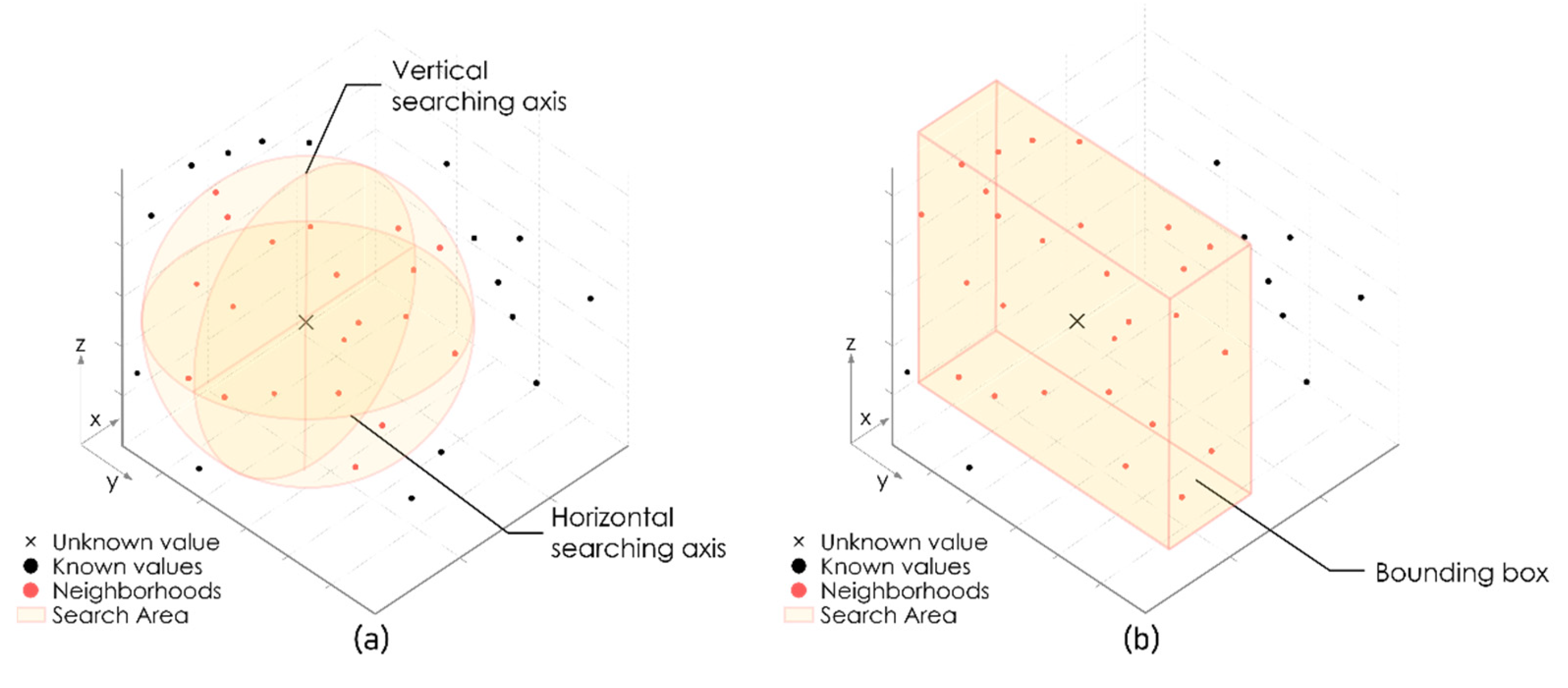
2.3.1. 3D Search Neighborhoods

Research on topology, represented by proximity, connectivity, and inclusivity, is becoming more important and more expanded as GIS is implemented from a data visualization tool to an analysis and decision-making support system [34]. 9IM (9 Intersection Model) is a model that determines the topology between binary objects (A–B) and was developed based on Egenhofer and Herring’s mathematical framework [35]. In addition, 9IM determines the eight spatial relationships (“Disjoint”, “Contains”, “Within”, “Equals”, “Touches”, “Overlaps”, “Covers”, and “Covered by”) through a 3 × 3 relationship matrix of three elements (Interior, Exterior, Boundary) in binary objects.
Since it was proposed, the 9IM framework has expanded into 3DE-9IM [36], DE-9IM [37], and 25IM [38] among others, and DE-9IM was adopted as ISO 19125-1 Geospatial International Standard Specification. The realization of a topology depends largely on a spatial data model. In 3D GIS, the standard data model on geometry adopted CityGML [39], and the standard data model on topology adopted IndoorGML [40], but they only deal with cases under traditional urban environments. Therefore, they are limited in being applied to other nonurban environments, such as subsurface, atmosphere, ocean, etc.
In 3D CAD systems, including GIS, B-rep (Boundary representation) is the most widely used computer graphic processing technique. B-rep also combines geometric primitives, such as node-0D, edge-1D, and face-2D to construct and express 3D objects, but does not store the topology of said object explicitly. Regardless, the reason why most 3D GIS implement B-rep is that it can immediately extract the topology between objects [41]. In this context, Ellul and Haklay proposed a method for the realization of integrating geometry and topology by implementing the 9-IM model in B-rep [42]. Therefore, this study proposed a 3D search neighborhood based on B-rep for developing a point interpolation in 3D space.
In this study, to search all directional neighborhoods, use the “Within3D” relationship with the observation data, which is included in the spheroid, generated from the unsampled location. Under the 3DE-9IM by Kim et al., the “Within3D” relationship between 3D spatial objects is defined as follows.
a. Within3D(b) ⇔ (dim(a) ≤ dim(b))∧
(INT(a) ∩ INT(b) ≠ ∅)∧
(INT(a) ∩ EXT(a) = ∅)∧
(BND(a) ∩ EXT(b) = ∅)
⇔ a. Relate(b, “TF***F***”)
Here, the search distance of the neighborhoods is the explicit radius of the spheroid. However, since the search distance in 3D space is formed not only in a horizontal but in a vertical direction, the spheroid is generated using two parameters in the minor and major axes (Figure 4a). Moreover, in order to enhance the performance of the 3D search neighborhoods technique suggested from the study, the neighborhoods search method using bounding box is also developed, which rapidly distinguishes neighbors within the search distance (Figure 4b). Through Figure 3 and Figure 4, it is able to compare how different the neighborhood is determined between the existing approach and the proposed 3D search neighborhood method.

2.3.2. Improved IDW Interpolation

This study applied linear interpolation by referring to the IDW function of Shepard [43]. The principle of IDW interpolation is to calculate the unknown values using the neighboring observation value and weight after determining the neighborhoods from the unsampled location. Here, the weight is set in inverse proportion to the power of the distance (Equation (4)).
λ i = j = 1 n 1 d i j p λ j j = 1 n 1 d i j p
where λ i   is the i th unknown value, n is the number of neighborhoods, λ j   is the j th known value, d i j   is distance from the location with i th unknown value to the location with j th known value and p is the power ( p > 0 , generally 2).
The distance is evaluated by the Euclidean distance in 3D vector space (Equation 5)).
d a , b = i = 1 n a i b i 2
where d   is distance, a i , b i   are point locations to calculate the distance between two points.
The final neighborhood is determined to be the neighborhood included in the search distance, or the N-number of neighborhoods closest to the unsampled location is used in IDW interpolation. However, since the nearest neighbors in the 3D observation data are densely populated in a vertical direction and can be mostly formed in a vertical direction, an elevation exaggeration factor is set to adjust the distance scale in a vertical and horizontal directions and is used as the search distance.
When the search distance is given as the fixed parameter, two search distances separated by horizontal and vertical directions are required, which are used as the explicit radius of the spheroid according to Section 2.3.1. Here, if no neighbor exists within the spheroid, ’NoData’ is returned.
In contrast, when determining the number of neighbors as the fixed parameter, the nearest neighbor from the estimated unsampled location is set and the interpolation is performed. In case the set neighbor is located too far away, the maximum search distance to the vertical and horizontal directions can be limited. In addition, if the number of neighbors given in the neighborhood count is not satisfactory, only the neighbors within the search distance should be used, and if no neighbor exists, “NoData” is returned.

3. Research Results

This section shows the five steps from the acquisition of borehole data to seismic liquefaction assessment, the development of an improved IDW algorithm, and 3D seismic liquefaction hazard mapping. This workflow was proposed so that different application systems could achieve consistent aims by inputting, processing, and outputting highly interoperable data formats (Figure 5), and Figure 6 shows the conceptual diagram in 3D mapping of estimation results using voxel.
  • Achieve borehole data, unify contents and format. (Microsoft Excel (Microsoft, Redmond, WA, USA));
  • Perform seismic liquefaction hazard assessment by using refined borehole data (MATLAB (MathWorks, Natick, MA, USA));
  • Apply improved IDW interpolation. However, when the estimated result consists of ‘NoData’, Perform IDW interpolation repeatedly on the analyzed result (Rhino/Grasshopper (Robert McNeel & Associate, Seattle, WA, USA));
  • Perform 3D seismic liquefaction hazard mapping based on the estimated results (ArcGIS Pro (Esri, Redlands, CA, USA));
  • Publish 3D web application by using mapping results (ArcGIS Online/WebApp Builder (Esri, Redlands, CA, USA)).

3.1. Experiment Data

The experiment data was taken from the 899 subsurface boreholes, collected in “Songpa-gu, Seoul” from the National Geotechnical Information Portal System (https://www.geoinfo.or.kr/ (accessed on 22 July 2022)). This data is the result of the geotechnical survey and is stored with the projected coordinate system (ESPG: 5186). Due to the characteristics of borehole data, it can be shown that they are densely populated on roads, railways, apartment complexes, or civil engineering and construction sites (Figure 7). The borehole data in the National Geotechnical Information Portal System include groundwater level, geologic structure, and standard penetration test results by depth. Here, while groundwater level is one of the key elements in liquefaction assessment, the groundwater level record in borehole data is the observation data at a specific time of the year and does not contain seasonal variations, such as flooding or drought seasons and thus affect the precision of liquefaction assessment. Therefore, this study determined the groundwater level of the study area using the data in the normal season from the National Groundwater Information Center (https://www.gims.go.kr/ (accessed on 22 July 2022)).

3.2. Result of Seismic Liquefaction Assessment

As a result of classifying 899 boreholes by depth, 9615 3D point data were created and these were used to assess FL in 2.2. Seven seismic waves, including the Gyeongju and Pohang earthquakes in South Korea, the Hokkaido earthquakes in Japan, and some earthquakes in the US, Greece, and Italy, were used to perform the subsurface response analysis and liquefaction assessment, and the mean value was used as the representative value. Additionally, the spectrum matching was performed for compliance with the Standard Design Response Spectrum corresponding to the return period of 2400 years, stipulated in the Common Applications of Seismic Design Code. Later, each borehole was divided into a 1 m gap by the geological information and groundwater level data for the detailed liquefaction assessment by depth, and over 20 m, it was divided into 3 m to conduct the liquefaction assessment.

3.3. Improved IDW Interpolation and Mapping

3.3.1. Development of an Improved IDW Interpolation Algorithm

In this study, the 3D search neighborhoods require generating and representing B-rep-based precise spheroid. 3D CAD systems can be divided largely into polygonal modeling and Non-Uniform Rational B-splines (NURBS) modeling. Polygonal modeling produces meshes by combining polygons (generally triangles) to express objects, which has the advantage of allowing for fast modeling but is limited in expressing curved surfaces. On the other hand, NURBS modeling is the way of creating curves with the Bézier curve and B-splines and generates a surface from these curves. It is widely used in the fields where precision modeling is required, such as ships, cars, and architecture, among others. Therefore, this section offers the results of the algorithm development using Rhinoceros® Grasshopper, which is a NURBS-based 3D CAD system, to realize the proposed IDW interpolation method.
The first stage of the algorithm is to adjust the parameters. The developed algorithm is divided into the case in which the search distance is given (fixed distance; FD) and the case in which the number of neighbors is given (number of points; NP). Such a division implements a main role in decision making whether to limit search ‘distance’ or to limit ‘number of neighbors’ when determinating the neighborhoods. For instance, it is possible to search a neighborhood within a fixed distance with a spheroid-based approach, but it is unable to strictly maintain the number of neighbors. Thus, FD has five parameters, horizontal search distance (V1), vertical search distance (V2), assessment height/depth (V3), elevation exaggeration factor (V4), and power (V5), while NP has seven parameters, the maximum search distance toggle (V1), the maximum horizontal search distance (V2), the maximum vertical search distance (V3), the number of neighbors (V4), assessment height/depth (V5), altitude exaggeration factor (V6), and power (V7).
In the second stage, the 3 D grid data by altitude is produced for storing interpolation results by the given FD−V3, FD−V4, or NP−V5, NP−V6 assessment height/depth parameters. To promote the applicability of the assessment result, the study set the grid origin and size identical to 250 m grid data offered by the National Geographic Information Institute (https://map.ngii.go.kr/ (accessed on 22 July 2022)), and the altitude was set to 1 m to 20 m under the subsurface based on the FL assessment standards.
The third stage Is to search for neighbors. In FD, the spheroid is formed using FD−V1 and FD−V2, and the Within3D relationship to the borehole data is processed. Later, the distance from the unsampled location to the borehole data that has the Within3D relationship is calculated, and the IDW processing is performed using FD−V5. Figure 8a shows the example of the application of the improved IDW interpolation with 250 m of the horizontal search distance, 2 m of the vertical search distance, 1 m of the assessment depth, 100 m of the elevation exaggeration factor, and 2 power as the parameters.
NP uses as the horizontal and vertical search distances the diagonal length of the assessment grid extent and NP−V3 if NP−V1 is false, or NP−V2 and NP−V3 if it is not. Later, a virtual 3D box is generated in the direction of X–Y–Z axes to the given maximum search distance, and through the Within3D relationship processing, the neighbor is selected. Here, the final neighbors for interpolation are selected for up to NP−V4 based on the distance in ascending order and using NP−V5, the IDW process is performed. Figure 8b shows the example of the application of the improved IDW interpolation with 250 m of the maximum horizontal search distance, 2 m of the maximum vertical search distance, 1 m of the assessment depth, 100 m of the elevation exaggeration factor, 12 of the maximum neighbor number and 2 power as the parameters. It is shown that as opposed to FD, one neighbor is added in the diagonal direction so that four neighbors are used in IDW interpolation.
In the final stage, an Excel spreadsheet, which includes the assessment grid point coordinate, the z coordinate to which the elevation exaggeration factor was applied, IDW interpolation result, liquefaction assessment grade, and the number of neighbors, is returned. Here, the grade is ‘High’ if the IDW interpolation result is less than 1, ‘Moderate’ if it is between 1 and 2, and ‘Low’ if it is 2 or above. Figure 9 shows the algorithm developed in this process.
Using the developed algorithm, 12,340 assessment grids and 9615 boreholes in Songpa-gu, Seoul were used in interpolation with different parameters by NP and FD, and the results are shown in Table 1. The area with NoData is the area with no borehole data around or is far from the assessment grid, and the result showed that in the study area, NP uses the nearest neighbors most, compared to FD, which searches for neighbors within the fixed distance, and could further reduce the frequency of NoData in the resulting outcome. However, such a difference is due to the different characteristics of the methodology, and thus, there is a limit over which to decide the criteria of the interpolation performance assessment based on the frequency of NoData alone. If data is widely distributed or the observation data is lacking, NP could be an alternative. However, as the estimation is performed using the value of too faraway neighbors, it is necessary to limit the suitable search distance, and if the data is sufficiently dense, FD could produce a better outcome.
Nevertheless, frequency of ‘NoData’ was minimized by performing interpolation repeatedly over the estimation results when the results include ‘NoData’ in this study (Table 2). As the result of the experiment, repeated interpolation was applied from a minimum of 2 to a maximum of 5 times to all the results, excluding NP−III, and it shows that as the search distance shortens, the repetition of interpolation increases.

3.3.2. Mapping of Seismic Liquefaction Assessment

For the 3D mapping of the seismic liquefaction assessment results, the Excel document generated from the interpolation results is converted into vector data format in GIS (Shapefile). Here, for the effective visualization of the assessment grid densely populated in a vertical direction, the vertical coordinates in the 3D point use the altitude on which the elevation exaggeration factor was reflected. Later, the 3D mapping is completed by creating a voxel cube for each 3D point location. By the risk grade, the color of the voxel cubes is set to red, yellow, or green according to the vulnerability attribute, and the size of the cube is set by the horizontal and vertical search distances set above (Figure 10).
The biggest differentiation of the nearest neighbors analysis approach which is the most simple method in determinating neighbors in a 3D environment (in this study NP−Ⅲ) and the suggested spheroid-based 3D search neighborhoods is that the estimation results of proposed method efficiently reflect the vertical and horizontal anisotropy (Figure 11). The nearest neighbors approach is highly effected by neighbors on horizontal directions, whereas the suggested method generates results that maintain the direction of the data that is distributed vertically.

3.3.3. Publishing 3D Web App

OGC I3S (indexed 3D Scene Layers) Standards were designed to stream SLPK (Scene Layer Package) that contains the most heterogeneous spatial data, such as KML, KMZ, Geodatabase, Multipatch, and Shapefile, friendly to the mobile or web environment based on modern web standards [44]. These standards allow for accessing 3D GIS services on mobile or web browsers without additional plugins and are used as a method to promote user accessibility and service interoperability. Thus, this study used Esri ArcGIS Pro to convert the 3D building model and the voxel data generated above to SLPK, and using ArcGIS Online, it developed an I3S-based 3D Web App (Figure 12). The background map is displayed in 2.5D system for visualization under the subsurface, and the voxel data with seismic liquefaction vulnerability were visualized under the surface to produce realistic scenes. Furthermore, through the filtering of the risk grade categorized above, the regions with liquefaction hazard mapping could be effectively browsed.

4. Summary and Conclusions

The study proposed an interpolation method for observation data collected in 3D, such as altitude, depth, or water level, and as an example, it showed the results of the seismic liquefaction hazard assessment and mapping using borehole data. As a result, the study showed that the interpolation of 3D observation data was possible through the integration of IDW, the most widely used interpolation method, and the B-rep-based topological relationship in 3D GIS. Such an approach is advantageous in the interpolation and visualization of various data observed in the real world and can contribute to the expansion of 3D GIS applications. The following is the proposal for improvement plans for the comparison and review of the developed outcomes to the previous research and further application to future research.
Concerning the 3D IDW interpolation, this study is significant in that it expanded the neighborhood search, the distance calculation, and the interpolation performed in the 2D space to the 3D space. However, the study did not quantitatively evaluate the results of the improved IDW interpolation, and therefore, it is necessary to discuss such results in the future.
Concerning 3D search neighborhoods, this study performed a searching topology relationship with the observed data by visualizing the spheroid or box according to the given search distance in the B-rep structure. This is an expansion of the 2D search neighborhoods to a 3D environment and was proposed by considering the characteristics of data densely populated in a vertical direction. A similar concept can be found in the Empirical Bayesian Kriging 3D offered by Esri [45]. This interpolation method determines neighbors by visualizing a sphere that has an identical distance to all axes, and based on the user’s definition, it can also determine neighbors by identifying sectors. Such an approach is used in identifying neighbors in an independent space and can be efficiently applied to the observation data affected by direction. Such an approach is used in identifying neighbors in an independent space and can be efficiently applied to the observation data affected by direction. For example, local atmospheric environment data has various directions of wind angles, and wind field estimation based on this data can be useful in various simulations [46].
Concerning seismic liquefaction hazard assessment, generally, it assesses FL to evaluate the occurrence of liquefaction by depth on one spot. However, in the case of the liquefaction hazard map that deals with a small-scale map, it uses the liquefaction potential index (LPI), which is produced by multiplying and integrating FL with the inverse weighting value of depth. Since LPI provides liquefaction potential on the ground surface, it can evaluate the liquefaction potential of facilities located on the ground. However, in South Korea, where underground space is actively used, it is necessary to conduct liquefaction potential assessments not only on facilities on the ground but also on underground facilities. Therefore, this study performed 3D liquefaction hazard mapping through improved interpolation based on FL by depth. Such 3D mapping results can be used as the criteria showing the subsurface liquefaction potential and also in selecting the target regions for an earthquake preparedness/response plan.
Concerning interpolation and mapping workflow, the study proposed the workflow aiming to integrate the functions of various S/W through the link among widely used file systems and standard data formats, such as Excel spreadsheet, Shapefile, and SLPK among others. While such an approach can be effectively used when no standard workflow exists, it is limited in terms of data duplication and S/W maintenance. Therefore, it is necessary to develop a 3D interpolation method that allows for integrated data processing and mapping in a single system.
Regarding processing performance, this study focused on the creation of precise B-rep objects and analyzing topology relationships via NURBS modeling, and therefore, the developed algorithm did not go through the optimization process. As such, when a large data set is input, writing results take a long time. Therefore, it is necessary to propose an improved algorithm with the concept of the 3D search neighborhoods from the perspective of algorithm performance.

Author Contributions

Conceptualization and methodology, S.S. and J.K.; data curation, K.P.; writing—original draft, J.K. and S.S.; writing—review and editing, J.H.; resources, J.H. and K.P. All authors have read and agreed to the published version of the manuscript.

Funding

This research was supported by the ‘A study on the advancement of building technology of tech-lead type liquefaction hazard map’ (20220056), the Key Project of the Korea Institute of Civil Engineering and Building Technology.

Institutional Review Board Statement

Not applicable.

Informed Consent Statement

Not applicable.

Data Availability Statement

Not applicable.

Acknowledgments

This research was conducted with the support of the ‘A study on the advancement of building technology of tech-lead type liquefaction hazard map’ (20220056), the Key Project of the Korea Institute of Civil Engineering and Building Technology.

Conflicts of Interest

The authors declare no conflict of interest.

References

  1. Arun, P.V. A comparative analysis of different DEM interpolation methods. Egypt. J. Remote Sens. Space Sci. 2013, 16, 133–139. [Google Scholar] [CrossRef] [Green Version]
  2. Li, L.; Losser, T.; Yorke, C.; Piltner, R. Fast inverse distance weighting-based spatiotemporal interpolation: A web-based application of interpolating daily fine particulate matter PM2.5 in the contiguous U.S. using parallel programming and k-d tree. Int. J. Environ. Res. Public Health 2014, 11, 9101–9141. [Google Scholar] [CrossRef] [PubMed]
  3. Hart, Q.J.; Brugnach, M.F.; Temesgen, B.; Rueda, C.; Ustin, S.L.; Frame, K. Daily reference evapotranspiration for California using satellite imagery and weather station measurement interpolation. Civil Eng. Environ. Syst. 2009, 26, 19–33. [Google Scholar] [CrossRef]
  4. Zhou, G.; Esaki, T.; Mitani, Y.; Xie, M.; Mori, J. Spatial probabilistic modeling of slope failure using an integrated GIS Monte Carlo simulation approach. Eng. Geol. 2013, 68, 373–386. [Google Scholar] [CrossRef]
  5. Aissiou, M.; Périé, D.; Gervais, J.; Trochu, F. Development of a progressive dual kriging technique for 2D and 3D multi-parametric MRI data interpolation. Comput. Methods Biomech. Biomed. Eng. Imag. Vis. 2013, 1, 69–78. [Google Scholar] [CrossRef]
  6. Widi, A.P.; Utomo, W.H.; Yulianto, J.P. Identification of Spatial Patterns of Food Insecurity Regions using Moran’s I (Case Study: Boyolali Regency). Int. J. Comput. Appl. 2013, 72, 54–62. [Google Scholar] [CrossRef]
  7. Birch, C.P.D.; Oom, S.P.; Beecham, J.A. Rectangular and hexagonal grids used for observation, experiment and simulation in ecology. Ecol. Model. 2007, 206, 347–359. [Google Scholar] [CrossRef]
  8. Yoon, J.H.; Li, Y.J.; Lee, M.S.; Jo, M.H. Deep Learning Drone Flying Height Prediction for Efficient Fine Dust Concentration Measurement. In Proceedings of the 13th International Conference on Ubiquitous Information Management and Communication (IMCOM), Phuket, Thailand, 4–6 January 2019; Lee, S., Ismail, R., Choo, H., Eds.; Springer: Cham, Swizterland, 2019; pp. 1112–1119. [Google Scholar]
  9. Sun, L.; Wei, Y.; Cai, H.; Yan, J.; Xiao, J. Improved fast adaptive IDW interpolation algorithm based on the borehole data sample characteristic and its application. J. Phys. Conf. Ser. 2019, 1284, 012074. [Google Scholar] [CrossRef] [Green Version]
  10. Sayre, R.G.; Wright, D.J.; Breyer, S.P.; Butler, K.A.; van Graafeiland, K.; Costello, M.J.; Harris, P.T.; Goodin, K.L.; Guinotte, J.M.; Basher, Z.; et al. A three-dimensional mapping of the ocean based on environmental data. Oceanography 2017, 30, 90–103. [Google Scholar] [CrossRef]
  11. Guo, J.; Wang, X.; Wang, J.; Dai, X.; Wu, L.; Li, C.; Li, F.; Liu, S.; Jessell, M.W. Three-dimensional geological modeling and spatial analysis from geotechnical borehole data using an implicit surface and marching tetrahedra algorithm. Eng. Geol. 2021, 284, 106047. [Google Scholar] [CrossRef]
  12. Nistor, M.M.; Rahardjo, H.; Satyanaga, A.; Hao, K.Z.; Xiaosheng, Q.; Sham, A.W.L. Investigation of groundwater table distribution using borehole piezometer data interpolation: Case study of Singapore. Eng. Geol. 2020, 271, 105590. [Google Scholar] [CrossRef]
  13. Pollack, H.N.; Smerdon, J.E. Borehole climate reconstructions: Spatial structure and hemispheric averages. J. Geophys. Res. Atmos. 2004, 109, D11106. [Google Scholar] [CrossRef]
  14. Iwasaki, T.; Arakawa, T.; Tokida, K.I. Simplified procedures for assessing soil liquefaction during earthquakes. Int. J. Soil Dyn. Earthq. Eng. 1984, 3, 49–58. [Google Scholar] [CrossRef]
  15. Lam, N.S. Spatial interpolation methods: A review. Am. Cartogr. 1983, 10, 129–150. [Google Scholar] [CrossRef]
  16. Comber, A.; Zeng, W. Spatial interpolation using areal features: A review of methods and opportunities using new forms of data with coded illustrations. Geogr. Compass 2019, 13, e12465. [Google Scholar] [CrossRef] [Green Version]
  17. Goodchild, M.F.; Lam, N.S.N. Areal interpolation: A variant of the traditional spatial problem. Geo-Processing 1980, 1, 297–312. [Google Scholar]
  18. Wright, J.K. A method of mapping densities of population with cape cod as an example. Geogr. Rev. 1936, 26, 103–110. [Google Scholar] [CrossRef]
  19. Lee, S.J.; Lee, S.W.; Hong, B.Y.; Eom, H.M.; Shin, H.S.; Kim, K.M. Representation of population distribution based on residential building types by using the dasymetric mapping in Seoul. J. Korea Spat. Inf. Soc. 2014, 22, 89–99. [Google Scholar] [CrossRef] [Green Version]
  20. Mitas, L.; Mitasova, H. Spatial Interpolation, In Geographical Information Systems: Principles, Techniques, Management and Applications; Longley, P., Goodchild, M.F., Maguire, D., Rhind, D., Eds.; Wiley: Hoboken, NJ, USA, 1999; pp. 481–492. [Google Scholar]
  21. Tobler, W.R.; Kennedy, S. Smooth multidimensional interpolation. Geogr. Anal. 1985, 17, 251–257. [Google Scholar] [CrossRef]
  22. Franke, R.; Nielson, G. Scattered Data Interpolation and Applications: A Tutorial and Survey. In Geometric Modelling: Methods and Applications; Hagen, H., Roller, D., Eds.; Springer: Berlin/Heidelberg, Germany, 1991; pp. 131–160. [Google Scholar]
  23. Watson, D.F. Contouring: A Guide to the Analysis and Display of Spatial Data; Pergamon: New York, NY, USA, 1992; pp. 101–162. [Google Scholar]
  24. Myers, D.E. Co-Kriging—New Developments. In Geostatistics for Natural Resources Characterization; Verly, G., David, M., Journel, A.G., Marechal, A., Eds.; Springer: Dordrecht, The Netherlands, 1984; pp. 295–305. [Google Scholar]
  25. Pilz, J.; Spöck, G. Why do we need and how should we implement Bayesian kriging methods. Stoch. Environ. Res. Risk Assess. 2008, 22, 621–632. [Google Scholar] [CrossRef]
  26. Krivoruchko, K. Empirical Bayesian kriging. Esri Press ArcUser 2012, 6–10. [Google Scholar]
  27. Chiles, J.P.; Delfiner, P. Geostatistics: Modeling Spatial Uncertainty, 2nd ed.; John Wiley & Sons: Hoboken, NJ, USA, 2012. [Google Scholar]
  28. Esri Homepage. Empirical Bayesian Kriging 3d. Available online: https://pro.arcgis.com/en/pro-app/2.8/help/analysis/geostatistical-analyst/what-is-empirical-bayesian-kriging-3d-.htm (accessed on 13 July 2022).
  29. Yang, L.; Achtziger-Zupančič, P.; Caers, J. 3D modeling of large-scale geological structures by linear combinations of implicit functions: Application to a large banded iron formation. Nat. Resour. Res. 2021, 30, 3139–3163. [Google Scholar] [CrossRef]
  30. Carr, J.C.; Beatson, R.K.; Cherrie, J.B.; Mitchell, T.J.; Fright, W.R.; McCallum, B.C.; Evans, T.R. Reconstruction and Representation of 3D Objects with Radial Basis Functions. In Proceedings of the 28th Annual Conference on Computer Graphics and Interactive Techniques, Los Angeless, CA, USA, 12–17 August 2001; pp. 67–76. [Google Scholar]
  31. Liu, Z.; Zhang, Z.; Zhou, C.; Ming, W.; Du, Z. An adaptive inverse-distance weighting interpolation method considering spatial differentiation in 3D geological modeling. Geosciences 2021, 11, 51. [Google Scholar] [CrossRef]
  32. Ji, Y.S.; Kim, H.S.; Lee, M.G.; Cho, H.I.; Sun, C.G. MLP-based 3D geotechnical layer mapping using borehole database in Seoul, South Korea. J. Korean Geotechn. Soc. 2021, 37, 47–63. [Google Scholar] [CrossRef]
  33. Korea Geotechnical Society. Explanation of Design Standard of Structure Foundation; CIR: Seoul, Korea, 2018. [Google Scholar]
  34. Ellul, C.; Haklay, M. Requirements for topology in 3D GIS. Trans. GIS 2006, 1, 157–175. [Google Scholar] [CrossRef]
  35. Egenhofer, M.; Herring, J. A Mathematical Framework for the Definition of Topological Relationships. In Proceedings of the 4th International Symposium on Spatial Data Handling, Zurich, Switzerland, 23–27 July 1990; pp. 803–813. [Google Scholar]
  36. Kim, S.H.; Kang, G.; Ryu, G.H. Design of three dimensional spatial topological relational operators. KIPS Trans. Part D 2003, 10D, 211–220. [Google Scholar] [CrossRef] [Green Version]
  37. Strobl, C. Dimensionally extended nine-intersection model (DE-9IM). In Encyclopedia of GIS; Shekahar, S., Xiong, H., Eds.; Springer: Berlin, Germany, 2008; pp. 240–245. [Google Scholar]
  38. Zhou, M.; Guan, Q. A 25-intersection model for representing topological relations between simple spatial objects in 3-D space. ISPRS Int. J. Geo-Inf. 2019, 8, 182. [Google Scholar] [CrossRef] [Green Version]
  39. OGC Homepage. City Geography Markup Language (CityGML) Part 1: Conceptual Model Standard. Available online: http://www.opengis.net/doc/IS/CityGML-1/3.0 (accessed on 20 August 2022).
  40. OGC Homepage. IndoorGML 1.1. Available online: http://www.opengis.net/doc/IS/indoorgml/1.1 (accessed on 20 August 2022).
  41. Boguslawski, P.; Gold, C.M.; Ledoux, H. Modelling and analysing 3D buildings with a primal/dual data structure. ISPRS J. Photogramm. Remote Sens. 2007, 66, 188–197. [Google Scholar] [CrossRef] [Green Version]
  42. Ellul, C.; Haklay, M. Using a B-Rep Structure to Query 9-Intersection Topological Relationships in 3d Gis–Reviewing the Approach and Improving Performance. In 3D Geo-Information Sciences; Lee, J., Zlatanova, S., Eds.; Springer: Berlin/Heidelberg, Germany, 2009; pp. 127–151. [Google Scholar]
  43. Shepard, D. A Two-Dimensional Interpolation Function for Irregularly Spaced Data. In Proceedings of the 1968 23rd ACM national conference, New York, USA, 27–29 August 1968; pp. 517–524. [Google Scholar]
  44. OGC Homepage. Indexed 3D Scene Layer (I3S) and Scene Layer Package (*.slpk) Format Community Standard Version 1.2. Available online: http://docs.opengeospatial.org/cs/17-014r8/17-014r8.html (accessed on 20 August 2022).
  45. Esri Homepage. 3D Search Neighborhoods. Available online: https://pro.arcgis.com/en/pro-app/2.8/help/analysis/geostatistical-analyst/3d-search-neighborhoods.htm (accessed on 30 August 2022).
  46. Li, Q.; Jia, H.; Qiu, Q.; Lu, Y.; Zhang, J.; Mao, J.; Fan, W.; Huang, M. Typhoon-Induced Fragility Analysis of Transmission Tower in Ningbo Area Considering the Effect of Long-Term Corrosion. Appl. Sci. 2022, 12, 4774. [Google Scholar] [CrossRef]
Figure 1. Neighborhood types in a grid system.
Applsci 12 11652 g001
Figure 2. Interpolation of a DEM: (a) Ordinary Kriging (spherical variogram); (b) IDW; (c) Regularized Spline; (d) Tension Spline.
Applsci 12 11652 g002
Figure 3. 3D search neighborhoods: (a) Constrained Delaunay triangle-based approach [31]; (b) Two search-grid surround boxes-based approach [9].
Applsci 12 11652 g003
Figure 4. Proposed approaches for 3D search neighborhoods: (a) Spheroid-based approach; (b) bounding box-based approach.
Applsci 12 11652 g004
Figure 5. Workflow of borehole data-based seismic liquefaction hazard assessment and mapping.
Applsci 12 11652 g005
Figure 6. Conceptual diagram of improved IDW results mapping.
Applsci 12 11652 g006
Figure 7. Borehole density in the study area.
Applsci 12 11652 g007
Figure 8. Limiting neighborhoods used for improved IDW: (a) Fixed search radius; (b) Fixed neighborhood counts.
Applsci 12 11652 g008
Figure 9. Improved IDW algorithm using 3D search neighborhoods.
Applsci 12 11652 g009
Figure 10. Improved IDW interpolation results: (a) Borehole data applied with elevation exaggeration factor; (b) NP−Ⅰ; (c) NP−Ⅱ; (d) NP−Ⅲ; (e) FD−Ⅰ; (f) FD−Ⅱ.
Applsci 12 11652 g010
Figure 11. Comparison of IDW interpolation results: (a) NP−Ⅲ; (b) FD−Ⅰ.
Applsci 12 11652 g011
Figure 12. 3D seismic liquefaction hazard web mapping application.
Applsci 12 11652 g012
Table 1. Summary of 1st interpolation results.
MethodParameterVulnerability
H-DistV-DistEXZNbrsLowModerateHighNoDataTotal
NP500 2100126589
(53.40%)
3094
(25.07%)
93
(0.75%)
2564
(20.78%)
12,340
(100%)
1000 2100128053
(65.26%)
4045
(32.78%)
105
(0.85%)
137
(1.11%)
12,340
(100%)
- -100128232
(66.71%)
4008
(32.48%)
100
(0.81%)
-12,340
(100%)
FD500 2100-5466
(44.29%)
3397
(27.53%)
54
(0.44%)
3423
(27.74%)
12,340
(100%)
1000 2100-5690
(46.11%)
6258
(50.71%)
7
(0.06%)
385
(3.12%)
12,340
(100%)
Table 2. Summary of final interpolation results.
MethodParameterVulnerability
H-DistV-DistEXZNbrsRepeatLowModerateHighNoDataTotal
NPI500 21001258476
(68.69%)
3759
(30.46%)
105
(0.85%)
-12,340
(100%)
II1000 21001228190
(66.37%)
4045
(32.78%)
105
(0.85%)
-12,340
(100%)
III- -10012-8232
(66.71%)
4008
(32.48%)
100
(0.81%)
-12,340
(100%)
FDI500 2100-57986
(64.72%)
4285
(34.72%)
69
(0.56%)
-12,340
(100%)
II1000 2100-26043
(48.97%)
6290
(50.97%)
7
(0.06%)
-12,340
(100%)
Publisher’s Note: MDPI stays neutral with regard to jurisdictional claims in published maps and institutional affiliations.

