
Parametric Equations and Polar Coordinates
Parametric Equations
Parametric equations are a set of equations in which the coordinates (e.g., [latex]x[/latex] and [latex]y[/latex]) are expressed in terms of a single third parameter.Learning Objectives
Express two variables in terms of a third variable using parametric equationsKey Takeaways
Key Points
- Parametric equations are useful for drawing curves, as the equation can be integrated and differentiated term-wise.
- A common example occurs in kinematics, where the trajectory of a point is usually represented by a parametric equation with time as the parameter.
- Equations can be converted between parametric equations and a single equation.
Key Terms
- coordinate: a number representing the position of a point along a line, arc, or similar one-dimensional figure

Parametric Example: One example of a sketch defined by parametric equations. Note that it is graphed on parametric axes.
Calculus with Parametric Curves
Calculus can be applied to parametric equations as well.Learning Objectives
Use differentiation to describe the vertical and horizontal rates of change in terms of [latex]t[/latex]Key Takeaways
Key Points
- Parametric equations are equations that depend on a single parameter.
- A common example comes from physics. The trajectory of an object is well represented by parametric equations.
- Writing the horizontal and vertical displacement in terms of the time parameter makes finding the velocity a simple matter of differentiating by the parameter time. Parameterizing makes this kind of analysis straight-forward.
Key Terms
- acceleration: the change of velocity with respect to time (can include deceleration or changing direction)
- displacement: a vector quantity which denotes distance with a directional component
- trajectory: the path of a body as it travels through space
Trajectories: A trajectory is a useful place to use parametric equations because it relates the horizontal and vertical distance to the time.
Polar Coordinates
Polar coordinates define the location of an object in a plane by using a distance and an angle from a reference point and axis.Learning Objectives
Use a polar coordinate to define a point with [latex]r[/latex] (distance from pole), and [latex]\theta[/latex](angle between axis and ray)Key Takeaways
Key Points
- Polar coordinates use a distance from a central point called a radial distance, usually specified as [latex]r[/latex].
- Polar coordinates use an angle measurement from a polar axis, which is usually positioned as horizontal and pointing to the right. Counterclockwise is usually positive.
- To convert from Polar coordinates to Cartesian coordinates, draw a triangle from the horizontal axis to the point. The [latex]r[/latex] coordinate is [latex]r \cos \theta[/latex] and the y coordinate is [latex]r \sin \theta[/latex].
Key Terms
- polar: of a coordinate system, specifying the location of a point in a plane by using a radius and an angle

Polar Coordinates: A set of polar coordinates. Note the polar angle increases as you go counterclockwise around the circle with 0 degrees pointing horizontally to the right.

Relation between Cartesian and Polar Coordinates: The [latex]x[/latex] Cartesian coordinate is given by [latex]r \cos \theta[/latex] and the [latex]y[/latex] Cartesian coordinate is given by [latex]r \sin \theta[/latex].
Area and Arc Length in Polar Coordinates
Area and arc length are calculated in polar coordinates by means of integration.Learning Objectives
Evaluate arc segment area and arc length using polar coordinates and integrationKey Takeaways
Key Points
- Arc length is the linear length of the curve if it were straightened out.
- The area is the size of the region defined by the curve radius and the angle and length of the connection lines enclosing the area.
- To calculate these dimensions, use integration over the angle.
Key Terms
- polar: of a coordinate system, specifying the location of a point in a plane by using a radius and an angle
Arc Length
If you were to straighten a curved line out, the measured length would be the arc length. Since it can be very difficult to measure the length of an arc linearly, the solution is to use polar coordinates. Using polar coordinates allows us to integrate along the length of the arc in order to compute its length. The arc length of the curve defined by a polar function is found by the integration over the curve [latex]r(\theta)[/latex]. Let [latex]L[/latex] denote this length along the curve starting from points [latex]A[/latex] through to point [latex]B[/latex], where these points correspond to [latex]\theta = a[/latex] and [latex]\theta = b[/latex] such that [latex]0 < b-a < 2 \pi[/latex]. The length of [latex]L[/latex] is given by the following integral: [latex-display]\displaystyle{L = \int_a^b \sqrt{r^2 + \left(\frac{dr}{d\theta}\right)^2} d\theta}[/latex-display] Solving this integral will give the length of the arc.
Arc Length: The curved lines bounding the region [latex]R[/latex] are arcs. Their length can be calculated with calculus. The area of the region [latex]R[/latex] can also be calculated by integration.
Arc Segment Area
To find the area enclosed by the arcs and the radius and polar angles, you again use integration. Let [latex]R[/latex] denote the region enclosed by a curve [latex]r(\theta)[/latex] and the rays [latex]\theta = a[/latex] and [latex]\theta = b[/latex], where [latex]0 < b-a < 2 \pi[/latex]. Then, the area of [latex]R[/latex] is: [latex-display]\displaystyle{\frac{1}{2} \int_a^b r^2 d\theta}[/latex-display] This result can be found as follows. First, the interval [latex][a, b][/latex] is divided into [latex]n[/latex] subintervals, where [latex]n[/latex] is an arbitrary positive integer. Thus [latex]\Delta \theta[/latex], the length of each subinterval, is equal to [latex]b-a[/latex] (the total length of the interval), divided by [latex]n[/latex], the number of subintervals. For each subinterval [latex]i = 1, 2, \cdots, n[/latex], let [latex]\theta_i[/latex] be the midpoint of the subinterval, and construct a sector with the center at the pole, radius [latex]r(\theta_i)[/latex], central angle [latex]\Delta \theta[/latex] and arc length [latex]r(\theta_i)\Delta\theta[/latex]. The area of each constructed sector is therefore equal to [latex-display]\displaystyle{\frac{1}{2} r^2 \Delta\theta}[/latex-display] And the total area is the sum of these sectors. An infinite sum of these sectors is the same as integration.Conic Sections
Conic sections are defined by intersections of cones with planes.Learning Objectives
Identify conic sections as curves obtained from the intersection of a cone with a planeKey Takeaways
Key Points
- Conic sections are curves obtained from an intersection of a cone with a plane.
- Graphs of quadratic equations in two variables are conic sections.
- Conic sections are important in astronomy: the orbits of two massive objects that interact according to Newton's law of universal gravitation are conic sections if their common center of mass is considered to be at rest.
Key Terms
- cone: a surface of revolution formed by rotating a segment of a line around another line that intersects the first line

Types of Conic Sections: There are three types of conic sections: 1.Parabola; 2. Ellipse; 3. Hyperbola.
Arc Length and Speed
Arc length and speed in parametric equations can be calculated using integration and the Pythagorean theorem.Learning Objectives
Calculate arc length by integrating the speed of a moving object with respect to timeKey Takeaways
Key Points
- Arc length is the length of a curve. To calculate it in parametric equations, employ the Pythagorean Theorem.
- Arc lengths can be calculated by adding up a series of infinitesimal lengths along the arc. To do this, set up an integral over the parameter.
- Speed is the rate of change of the arc length with respect to time. The derivatives of [latex]x[/latex] and [latex]y[/latex] with respect to time are plugged into the Pythagorean Theorem to give the speed of an object traveling in an arc.
Key Terms
- Pythagorean Theorem: A theorem stating that the hypotenuse of a right triangle is equal to the square root of the sum of the square of the other two sides
- curve: a simple figure containing no straight portions and no angles
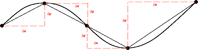
Approximating Arc Length with Hypotenuses: The length of a curve can be approximated by using a series of right triangles with the hypotenuses lying along the curve. The smaller the triangles one uses, the closer the approximation will be.
Conic Sections in Polar Coordinates
Conic sections are sections of cones and can be represented by polar coordinates.Learning Objectives
Identify types of conic sections using polar coordinatesKey Takeaways
Key Points
- Conic sections are the intersections of cones with a plane.
- The three types of conic sections are the hyperbola, parabola, and ellipse.
- Polar coordinates offer us a useful way of representing conic sections.
Key Terms
- cone: a surface of revolution formed by rotating a segment of a line around another line that intersects the first line
- hyperbola: a conic section formed by the intersection of a cone with a plane that intersects the base of the cone and is not tangent to the cone
Licenses & Attributions
CC licensed content, Shared previously
- Curation and Revision. Provided by: Boundless.com License: CC BY-SA: Attribution-ShareAlike.
CC licensed content, Specific attribution
- Parametric equations. Provided by: Wikipedia Located at: https://en.wikipedia.org/wiki/Parametric_equations. License: CC BY-SA: Attribution-ShareAlike.
- coordinate. Provided by: Wiktionary License: CC BY-SA: Attribution-ShareAlike.
- Parametric equations. Provided by: Wikipedia License: CC BY: Attribution.
- Parametric equation. Provided by: Wikipedia License: CC BY-SA: Attribution-ShareAlike.
- acceleration. Provided by: Wiktionary License: CC BY-SA: Attribution-ShareAlike.
- displacement. Provided by: Wiktionary License: CC BY-SA: Attribution-ShareAlike.
- trajectory. Provided by: Wiktionary License: CC BY-SA: Attribution-ShareAlike.
- Parametric equations. Provided by: Wikipedia License: CC BY: Attribution.
- Trajectory. Provided by: Wikipedia License: CC BY: Attribution.
- Polar coordinate system. Provided by: Wikipedia License: CC BY-SA: Attribution-ShareAlike.
- polar. Provided by: Wiktionary License: CC BY-SA: Attribution-ShareAlike.
- Parametric equations. Provided by: Wikipedia License: CC BY: Attribution.
- Trajectory. Provided by: Wikipedia License: CC BY: Attribution.
- Polar coordinate system. Provided by: Wikipedia License: CC BY: Attribution.
- Polar coordinate system. Provided by: Wikipedia License: CC BY: Attribution.
- Polar coordinate system. Provided by: Wikipedia License: CC BY-SA: Attribution-ShareAlike.
- Polar coordinate system. Provided by: Wikipedia License: CC BY-SA: Attribution-ShareAlike.
- polar. Provided by: Wiktionary License: CC BY-SA: Attribution-ShareAlike.
- Parametric equations. Provided by: Wikipedia License: CC BY: Attribution.
- Trajectory. Provided by: Wikipedia License: CC BY: Attribution.
- Polar coordinate system. Provided by: Wikipedia License: CC BY: Attribution.
- Polar coordinate system. Provided by: Wikipedia License: CC BY: Attribution.
- Polar coordinate system. Provided by: Wikipedia License: CC BY: Attribution.
- Conic section. Provided by: Wikipedia License: CC BY-SA: Attribution-ShareAlike.
- cone. Provided by: Wiktionary License: CC BY-SA: Attribution-ShareAlike.
- Parametric equations. Provided by: Wikipedia License: CC BY: Attribution.
- Trajectory. Provided by: Wikipedia License: CC BY: Attribution.
- Polar coordinate system. Provided by: Wikipedia License: CC BY: Attribution.
- Polar coordinate system. Provided by: Wikipedia License: CC BY: Attribution.
- Polar coordinate system. Provided by: Wikipedia License: CC BY: Attribution.
- Conic section. Provided by: Wikipedia License: CC BY: Attribution.
- Arc length. Provided by: Wikipedia License: CC BY-SA: Attribution-ShareAlike.
- Boundless. Provided by: Boundless Learning License: CC BY-SA: Attribution-ShareAlike.
- curve. Provided by: Wiktionary Located at: https://en.wiktionary.org/wiki/curve. License: CC BY-SA: Attribution-ShareAlike.
- Parametric equations. Provided by: Wikipedia License: CC BY: Attribution.
- Trajectory. Provided by: Wikipedia License: CC BY: Attribution.
- Polar coordinate system. Provided by: Wikipedia License: CC BY: Attribution.
- Polar coordinate system. Provided by: Wikipedia License: CC BY: Attribution.
- Polar coordinate system. Provided by: Wikipedia License: CC BY: Attribution.
- Conic section. Provided by: Wikipedia License: CC BY: Attribution.
- Arc length. Provided by: Wikipedia License: CC BY: Attribution.
- Conic section. Provided by: Wikipedia License: CC BY-SA: Attribution-ShareAlike.
- hyperbola. Provided by: Wiktionary License: CC BY-SA: Attribution-ShareAlike.
- cone. Provided by: Wiktionary License: CC BY-SA: Attribution-ShareAlike.
- Parametric equations. Provided by: Wikipedia License: CC BY: Attribution.
- Trajectory. Provided by: Wikipedia License: CC BY: Attribution.
- Polar coordinate system. Provided by: Wikipedia License: CC BY: Attribution.
- Polar coordinate system. Provided by: Wikipedia License: CC BY: Attribution.
- Polar coordinate system. Provided by: Wikipedia License: CC BY: Attribution.
- Conic section. Provided by: Wikipedia License: CC BY: Attribution.
- Arc length. Provided by: Wikipedia License: CC BY: Attribution.
